Study of Urban Heat Islands Using Different Urban Canopy Models and Identification Methods

Abstract

This work aims to compare the performance of the single‑(SLUCM) and multilayer (BEP-Building effect parameterization) urban canopy models (UCMs) coupled with the Weather Research and Forecasting model (WRF), along with the application of two urban heat island (UHI) identification methods. The identification methods are: (1) the “classic method”, based on the temperature difference between urban and rural areas; (2) the “local method” based on the temperature difference at each urban location when the model land use is considered urban, and when it is replaced by the dominant rural land use category of the urban surroundings. The study is performed as a case study for the city of Lisbon, Portugal, during the record-breaking August 2003 heatwave event. Two main differences were found in the UHI intensity (UHII) and spatial distribution between the identification methods: a reduction by half in the UHII during nighttime when using the local method; and a dipole signal in the daytime and nighttime UHI spatial pattern when using the classic method, associated with the sheltering effect provided by the high topography in the northern part of the city, that reduces the advective cooling in the lower areas under prevalent northern wind conditions. These results highlight the importance of using the local method in UHI modeling studies to fully isolate urban canopy and regional geographic contributions to the UHII and distribution. Considerable improvements were obtained in the near‑surface temperature representation by coupling WRF with the UCMs but better with SLUCM. The nighttime UHII over the most densely urbanized areas is lower in BEP, which can be linked to its larger nocturnal turbulent kinetic energy (TKE) near the surface and negative sensible heat (SH) fluxes. The latter may be associated with the lower surface skin temperature found in BEP, possibly owing to larger turbulent SH fluxes near the surface. Due to its higher urban TKE, BEP significantly overestimates the planetary boundary layer height compared with SLUCM and observations from soundings. The comparison with a previous study for the city of Lisbon shows that BEP model simulation results heavily rely on the number and distribution of vertical levels within the urban canopy.

1. Introduction

The urban heat island (UHI) effect is one of the most studied phenomena induced by human activities on local climate [1] and can be described as a positive thermal anomaly in urban areas with respect to their rural surroundings. Consequently, larger temperature differences between urban and rural environments lead to higher UHI intensity (UHII). On average, the UHII tends to be greater at night, under calm synoptic and clear‑sky conditions [1,2], although in some cases, urban cold islands (UCIs) can occur during the day [3].

Several factors contribute to the occurrence of UHIs. The distinct radiative, aerodynamic, and thermodynamic properties of urban and rural surfaces are normally the main causes [4,5]. The urban materials, with lower reflectivity and high thermal inertia, tend to absorb large amounts of shortwave radiation energy during the day, which is later released as longwave radiation and sensible heat during the night. Characteristics such as buildings geometry and road width can influence and reduce the sky view factor in urban canyons, causing radiation trapping, while augmenting the exposed area for radiation absorption during the beginning and end of the day [6,7,8,9]. Additionally, urban environments are characterized by the lack of vegetation and the presence of large areas of impervious surfaces that can reduce soil evapotranspiration (i.e., evaporation from soil and vegetation) [10,11,12,13,14,15]. Geographical factors, such as altitude, topography, and proximity of water bodies, have a great influence on the UHII [16]. Lastly, the number of inhabitants, city size, and the resulting anthropogenic heat release (traffic, air conditioning systems, human metabolism, and burning of heating fuels) are also important [1,16,17,18,19].

UHIs can be measured at the soil, surface, near-surface, or any height within the urban and planetary boundary layers [20]. Most of the existing studies focus on surface and near-surface analysis by applying a broad range of techniques and measuring methods. Depending on the type of UHI, data from ground-based meteorological stations (including fixed and transient), satellites (through remote sensing), airplanes, radiosondes, and meteorological models coupled with urban canopy models (UCMs) are used to access UHII and distribution [4].

Regarding UHI studies, Lowry (1977) [21] suggests that estimates and assumptions of urban effects on local and regional climate should only be accepted with confidence if accounting for preurban and normalized synoptic weather conditions, which raises questions about the use of traditional methods on the identification of UHIs. In this respect, Georgescu et al. (2011) [22] used the Weather Research and Forecasting (WRF) model coupled with the Single‑Layer Urban Canopy Model (SLUCM) to study the influence of the semiarid surrounding environment of the Phoenix metropolitan area on the city’s UHI during July 1979, 1989, and 1994. The authors performed three types of simulations experiments where: (1) the contemporary land use is considered; (2) the semiarid surrounding biome of the city is replaced with a temperate broadleaf forest biome; (3) the land use anthropogenic pixels are removed and replaced with native vegetation. The direct comparison between results from (3) and (1) enabled the assessment of anthropogenic landscape influence on UHI, while the comparison between results from (1) and (2) allowed the assessment of the impact of the surrounding environment on the city’s UHI. Similarly, Ma et al. (2017) [23] explored the relative contribution of urban canopy effects and anthropogenic heat fluxes on Sydney’s urban climate using the WRF model coupled with SLUCM. The authors performed different simulations for July and December of 2007, 2008, and 2009 to isolate the impacts of anthropogenic heat and urban canopy effects on the city UHI. The impacts of anthropogenic heat on the UHI are obtained through the comparison between simulations with and without anthropogenic heat, while urban canopy effects were identified by comparing simulations with contemporary land use with simulations where the urban land use categories were replaced with natural vegetation.

Aside from methodology aspects, various studies indicate the existence of synergistic interactions between UHI and heatwaves that can further exacerbate their combined effects in comparison with nonheatwave periods [2,24,25,26]. This is particularly worrying since future climate projections show an aggravation of heat-related risks resulting from UHIs during heatwaves events, due to the increase in future heatwaves intensity, frequency, and duration [27,28]. For the particular case of the city of Lisbon (Portugal), Rocha et al. (2020) [29] studied the climatic changes of various heatwave metrics for the mid- (2046–2065) and long-term future (2081–2100) with respect to the present climate (1986–2005) using WRF model regional climate simulations and an ensemble of models from the EURO‑CORDEX project [30], under the RCP8.5 greenhouse gases emission scenario. Their results show an increase in the number of heatwave days in the mid- and long-term future of around four and six times, respectively, along with an increase in the heatwave duration, intensity, and average maximum temperature.

Although computationally demanding, high‑resolution UHI simulations using regional atmospheric models coupled with UCMs can be useful if applied to high impact events such as heatwaves. Hence, in this study, we use the WRF model coupled with two different UCMs available in the WRF modeling system—the SLUCM and the Building Effect Parameterization (BEP) multilayer model—to estimate the intensity and distribution of the near-surface (i.e., at two-meter height) UHI in the Lisbon metropolitan area during the record‑breaking August 2003 European heatwave event [31,32]. The UHI is identified using two distinct methodologies: firstly, the “classic method”, which compares the differences between urban and rural sites temperatures; and secondly, the “local method”, which compares urban and rural temperature differences at urban locations using the results of simulations with the contemporary land use and simulations where the urban categories in the model’s land use map were removed and replaced with natural vegetation. By applying the local method, we fully eliminate the portion of the UHI associated with local physiography. Thus, the UHII and distribution only depends on urban geometry and on the characteristics of the surface materials.

Despite the existence of previous studies on the Lisbon UHI that provide a reasonable overview of its spatial and temporal variability using both statistical and deterministic approaches, they are based on the urban‑rural points measurement approach that lacks the spatial detail of high‑resolution model simulations. Furthermore, the methodologies used to map the UHI thermal patterns can be ambiguous and difficult to implement. For instance, Alcoforado and Andrade (2006) [33], using transect measurements and data from meteorological stations, applied a stepwise multiple regression approach to model the relationship between near‑surface air temperature, various parameters associated with local geography (e.g., local topography and distance to the Tagus river), and different urban geometry features. The best multiple regression predictors, combined with geographic information system techniques, were used to draw thermal maps of the nocturnal UHI. Later, Lopes et al. (2013) [34] and Alcoforado et al. (2014) [35] used hourly data from a mesoscale meteorological network (for the period between 2004 and 2012) to study the relationship between Lisbon’s urban thermal patterns and local wind regimes and to statistically study the UHI for applying climatic guidelines, respectively. Both studies conclude that, during the period of analysis, the UHII can reach up to 6 °C during some summer afternoons, evenings, and nights and median values of approximately 2 °C and 1.5 °C during the night and day periods, respectively. Higher UHII occur particularly under light wind conditions for north, north‑western, and south‑western wind regimes, while for wind speeds over 8 m s⁻¹ the UHI is inhibited. In a recently published study, Oliveira et al. (2021) [36] used hourly air temperature measurements from a mesoscale observation network in Lisbon, to establish the relationship between the region’s background weather and the UHI during summer heatwave and nonheatwave conditions, for the period between 2004 and 2015. Out of the 49 heatwaves identified during the 11‑year period, 37 occurred under near‑surface northern wind conditions, with UHII median values frequently reaching values lower than −1 °C during the day (i.e., UCI) and 1.5 °C during the night. Heatwaves occurring under such wind conditions revealed higher maximum temperature, thermal amplitude, and UHII. The latter was found to be controlled by the sheltering effect provided by the high topography of the northern part of the city. No evidence of synergistic interactions between UHII and higher temperatures was found, since the UHII was approximately the same when comparing heatwave with nonheatwave days.

Ultimately, this study aims to compare the application of two different UCMs, SLUCM and BEP, and two UHI identification methods, classic and local, in the characterization and investigation of UHI events. As a case study, the present work focuses on the Lisbon UHI that occurred during the August 2003 heatwave event. To the authors’ knowledge, this study compares for the first time classic and local methods applied with two different UCMs, providing an important side‑by‑side assessment of their influence on the dynamical and thermal aspects of UHIs. This work serves as a framework to evaluate the best WRF model configuration and identification method to be used in future UHI studies where the impacts of the city’s growth, anthropogenic heat, and irrigation of urban green spaces can be accessed for future heatwaves.

This article is structured as follows: Section 2 provides a description of the data and methods used, Section 3 provides the obtained results and discussion, and Section 4 summarizes the main conclusions.

2. Materials and Methods

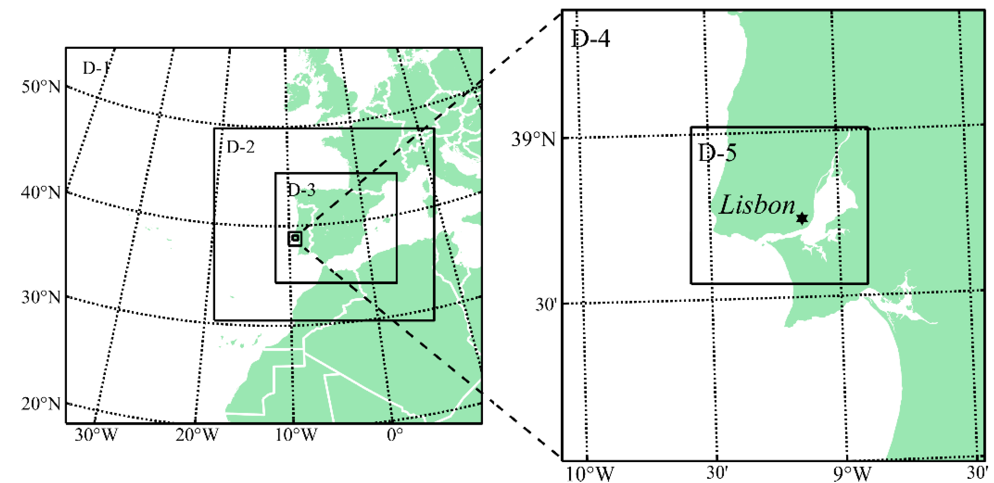
2.1. Model Setup and Description

The numerical simulations of the Lisbon UHI for the August 2003 heatwave event were performed using the WRF model version 3.9 [37]. WRF is a fully compressible and nonhydrostatic model, with terrain‑following vertical coordinates and a multiplicity of physics parameterization options. The model has been frequently used in operational numerical weather prediction, regional climate, hydrology, wildland fires, hurricanes, and UHI studies [38].

The ERA‑Interim reanalysis data from the European Centre for Medium‑Range Weather Forecasts (ECMWF) [39] were used to force the model in its initial and boundary conditions. The forcing data were obtained with a horizontal resolution of 0.75° × 0.75°, in 37 pressure levels, and provided to the model with six-hourly frequency. A configuration of five nested domains (Figure 1) was applied for the dynamical downscaling of the ERA‑Interim fields. The first three domains are the same as the ones used in the climatic simulations performed by Marta‑Almeida et al. (2016) [40] over the Iberian Peninsula, with horizontal grid spacing of 81 km (D‑1: 60 × 55 grid cells), 27 km (D‑2: 94 × 55 grid cells), and 9 km (D‑3: 154 × 139 grid cells). A further set of two nested domains, centered in Lisbon metropolitan area, with horizontal resolutions of 1 km (D‑4: 145 × 154 grid cells) and 333 m (D‑5: 181 × 160 grid cells), were added. The model ran in a two‑way nesting mode, with sea surface temperature update every six hours and spectral‑nudging in D‑1 for wavelengths larger than 1000 km [41], for the period between July 28 and August 2. The top of the model was defined at 50 hPa and the first 24 h of simulation were discarded due to model spin-up; thus, only the period between July 29 and August 2 was considered for the analysis. Vertical velocity damping was applied to reduce model instability in the higher resolution domains, where sudden changes in topography can produce unrealistic vertical velocities. The ERA‑Interim soil temperature and moisture fields were provided to the model at four levels. Although a longer model spin-up period than 24‑h seems reasonable for initializing soil properties, Jacobs et al. (2017) [42] has shown that the model‑predicted near‑surface urban temperature during heatwave conditions significantly improves when using a 24‑h spin‑up period for the soil moisture initialization instead of a longer period. However, it was also shown by the same author and by Xue et al. (2017) [43], that WRF model simulations initialized with ERA‑interim reanalysis might be subject to large bias regarding soil moisture and soil temperature. Future improvements to this study model’s setup may include the use of the much‑improved ERA‑5 reanalysis data as initial and lateral boundary conditions [44].

The physical parameterizations used in the model simulations were: WRF Single‑Moment 6‑class microphysics scheme [45]; Dudhia shortwave radiation scheme [46]; Rapid Radiative Transfer Model (RRTM) longwave radiation model [47]; Revised MM5 surface model [48]; BouLac planetary boundary layer model [49]; Noah Land Surface Model [50], and the Grell‑Freitas cumulus scheme [51]. Since the dynamic and thermodynamic effects associated with convective and shallow clouds can be explicitly resolved in the finer grid scales, the cumulus parameterization was turned off in domains D‑4 and D‑5 [37].

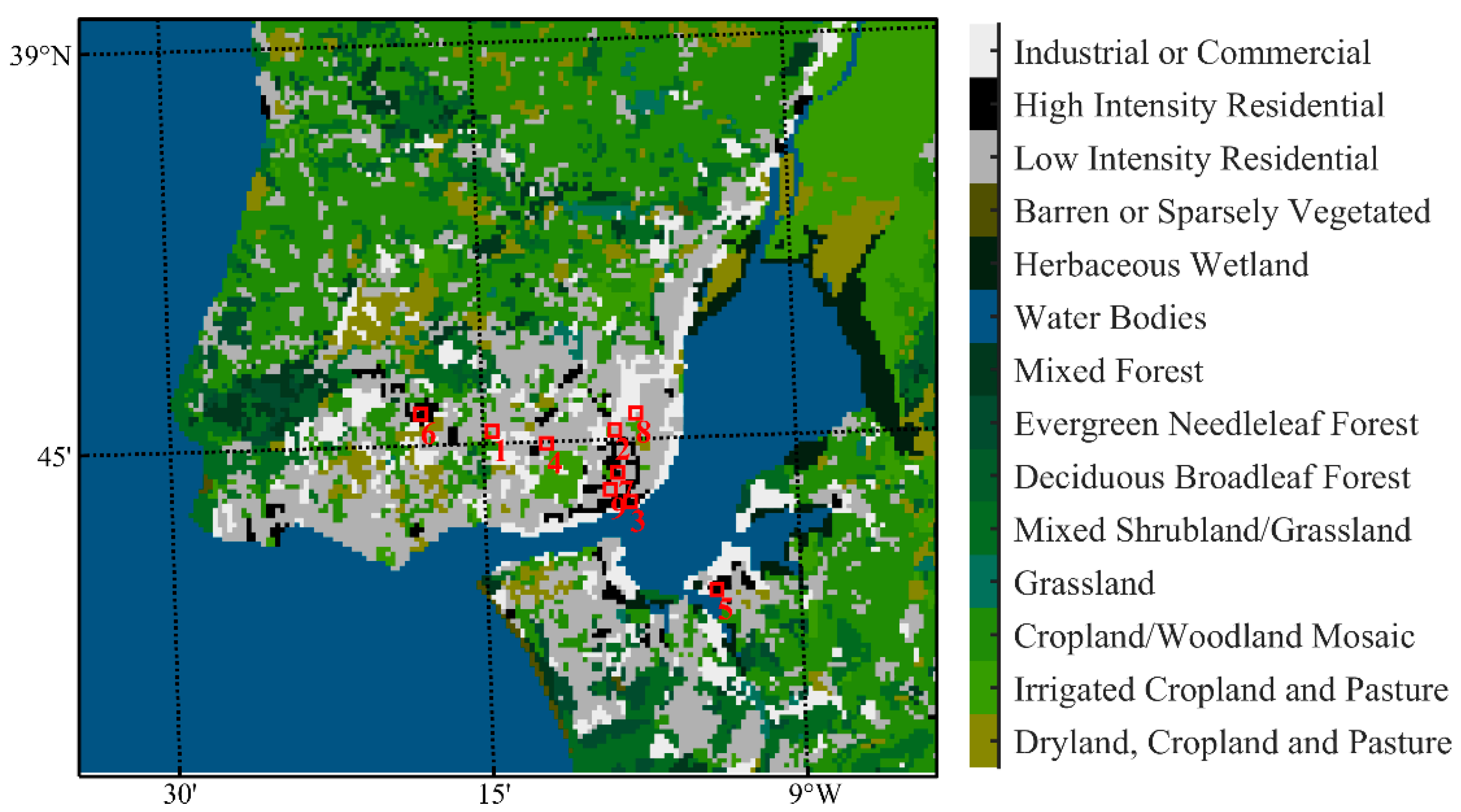
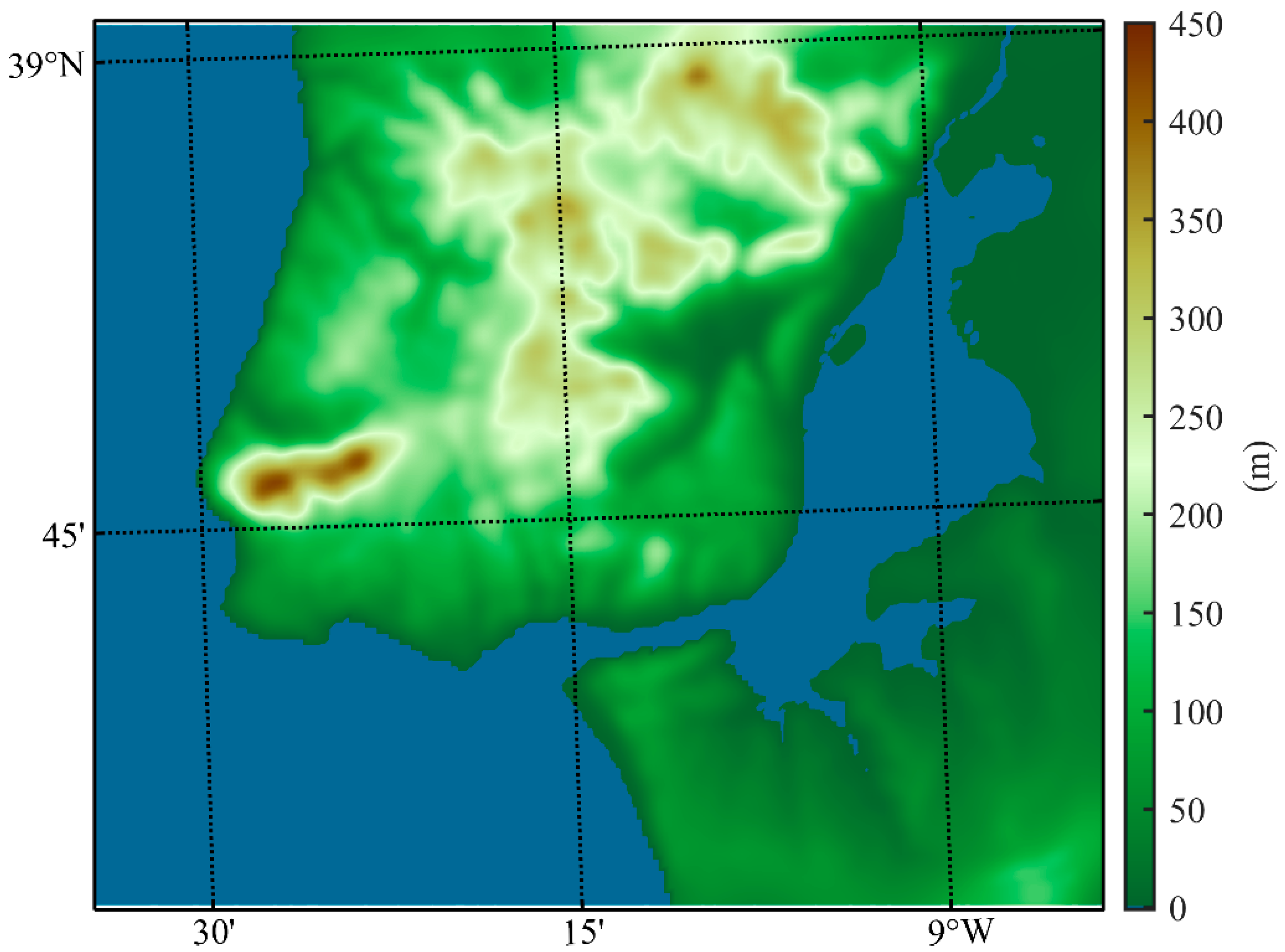
2.1.1. Topography and Land Use Data

For a better representation of the local topography and land use in the model grid, the standard database included in the WRF distribution was replaced by data from the NASA’s Shuttle Radar Topography Mission (SRTM) [52] and from the Coordination of Information on the Environment (CORINE) Land Cover [53] for the year of 2012 (hereafter referred as CLC2012), with a horizontal resolution of approximately 90 m and 100 m, respectively. The CLC2012 data was reclassified from its 44 categories into the United States Geological Survey (USGS) 33‑category (USGS33) classification system used by the WRF model, following the methodology described by Pineda et al. (2004) [54]. Since Pineda et al. (2004) [54] reclassification is based on USGS 24‑category (USGS24), which considers only one urban category, changes were made in order to include the three urban classes available in USGS33. The use of USGS33 allows for a better representation of the urban features, by considering three distinct urban categories: low intensity residential (LIR), high intensity residential (HIR), and industrial or commercial (IC). A summary of the equivalence between CLC2012 and USGS33 categories can be found in Table S1 (adapted from Pineda et al. (2004) [54] and Carvalho et al. (2017) [55]) of the Supplementary Material. In this study, the CLC2012 category 10 (i.e., green urban areas) was reclassified to the USGS category 3 (i.e., irrigated Cropland and Pasture) following the same methodology as Carvalho et al. (2017) [55]. Although the use of the 100 m resolution CLC2012 data represents an improvement relatively to the standard USGS dataset, derived from the Advanced Very High Resolution Radiometer (AVHRR) satellite data with 1 km spatial resolution, there are other land use datasets that provide a more consistent and detailed depiction of the different urban classes. Future work could involve the inclusion of a recently made available land use map for the city of Lisbon, based on the Local Climate Zones (LCZs) classification system [56], and developed by Oliveira et al. (2020) [57]. The use of LCZs should provide a better spatial resolution and accuracy in representing urban densities.

Figure 2 shows the model land use map in domain D‑5, together with the location of the nine meteorological stations used for the model validation which are installed and operated by the Portuguese National Weather Service (Instituto Português do Mar e da Atmosfera, IPMA). The representation of the topographic data for domain D‑5 is shown in Figure 3.

2.1.2. Urban Canopy Models

To accurately represent the processes associated with the exchange of momentum, heat, and moisture in the urban environment, the WRF model was coupled with two UCMs available in its modeling system, namely the single‑layer urban canopy model (SLUCM), developed by Kusaka et al. (2001) [58] and later modified by Kusaka and Kimura (2004) [59], and the multilayer building effect parameterization (BEP), developed by Martilli et al. (2002) [60]. These UCMs are coupled with the Noah LSM through the urban fraction parameter ($F$). Heat fluxes and temperatures from natural surfaces are computed by the Noah LSM, while the UCMs compute the fluxes and temperatures over artificial surfaces [59,61]. As an example, the total estimated grid‑scale surface latent heat flux (LH) is obtained as follows:

$$\mathrm{LH}=F_{urb}\times L{H}_{urb}+F_{veg}\times L{H}_{veg}$$

(1)

where $F_{urb}$ and $F_{veg}$ are the urban and vegetation fractions in a model grid cell, and $L{H}_{urb}$ and $L{H}_{veg}$ are the latent heat fluxes over vegetated and urban surfaces, respectively. The same procedure is applied for other surface variables such as surface sensible heat flux (SH), ground heat flux (GRD), upward longwave radiation, albedo, emissivity, and friction velocity, while surface skin temperature (TSK) is calculated as the averaged value of natural and artificial surfaces temperature multiplied by their areal coverage [61].

This information is passed to the PBL scheme through the surface model. The surface model computes the heat transfer coefficients for heat and momentum, while the computation of the heat transfer coefficient for moisture is made by the PBL scheme and given to the surface model. Based on these heat transfer coefficients the Noah LSM computes the heat and moisture fluxes, passing them to the PBL scheme for the computation of the flux convergence and turbulent kinetic energy (TKE) [48,49,50].

In SLUCM the urban geometry is represented by two‑dimensional infinitely long street canyons with different orientations (simplified geometry), but the radiation treatment is done three‑dimensionally by taking into consideration the effects of radiation trapping, reflection and shadowing, the diurnal variation of the azimuth solar angle, and the estimation of surface temperature and fluxes on vertical walls, roads, and roofs. Additionally, SLUCM assumes a prescribed exponential wind profile within the urban canopy and an option for the inclusion of anthropogenic latent and sensible heat diurnal cycle profiles [62]. In BEP the urban geometry is represented by three‑dimensional surfaces which allows the computation of heat and momentum sources and sinks at different levels of the urban canopy. As in SLUCM, all the radiative effects within the urban canyons are considered, as well as the effect of the different urban surfaces on momentum, TKE, and potential temperature [61]. BEP is the only urban parameterization option used in this study that directly interacts with the BouLac PBL scheme through the introduction of a source term in the TKE equation calculations within the urban canopy, and through the modification of the turbulent length scales to account for the presence of buildings. While SLUCM and BEP provide options to account for anthropogenic heating effects, they are not considered in this study, since these effects will be addressed separately in a future work. Therefore, the analysis presented here is based on the impact of the urban canopy effects on the UHI intensity and distribution.

Although the coupling of SLUCM and BEP with WRF is done through the Noah LSM, by activating the namelist.input configuration file option sf_urban_physics = 1 or = 2, respectively, deactivating this option (i.e., sf_urban_physics = 0) does not mean that urban surfaces effects are not considered. This is because, by default, the Noah LSM includes a bulk urban parameterization (Noah bulk) that represents zero‑order effects of the urban surfaces using parameters such as: roughness length, that represents turbulence generated by roughness elements and drag caused by buildings; surface albedo, that represents shortwave radiation trapping in the urban canyons; volumetric heat capacity for walls, roofs, and roads, which are assumed to be concrete or asphalt; soil thermal conductivity to represent heat storage in building and roads; and reduced urban fraction to represent the reduction of evapotranspiration [61]. These parameters are also used by the SLUCM and BEP models.

All the UCM models used in this study recognize the three urban categories available from USGS33 classification system. The thermal parameters defined for each UCM are presented in

Table 1. Values of the thermal parameters used in SLUCM and BEP urban canopy models.

Thermal Parameters	Urban Canopy Model
	SLUCM	BEP
CAPR: Heat capacity of the roof (106 J m−3 K−1)	1
CAPB: Heat capacity of the building wall (106 J m−3 K−1)	1
CAPG: Heat capacity of the ground (road) (106 J m−3 K−1)	1.4
AKSR: Thermal conductivity of the roof (106 J m−3 K−1)	0.67
AKSB: Thermal conductivity of the building wall (106 J m−3 K−1)	0.67
AKSG: Thermal conductivity of the ground (road) (106 J m−3 K−1)	0.4004
ALBR: Surface albedo of the roof (fraction)	0.2
ALBB: Surface albedo of the building wall (fraction)	0.2
ALBG: Surface albedo of the ground (road) (fraction)	0.2
EPSR: Surface emissivity of the roof (-)	0.9
EPSB: Surface emissivity of the building wall (-)	0.9
EPSG: Surface emissivity of the ground (road) (-)	0.95

, while the geometric parameters (i.e., building height, roof, and road widths) and the urban fraction for each urban category and UCM are defined in

Table 2. Geometric parameters and urban surface fraction defined for each urban category and urban canopy model.

Characteristic	Urban Class	Urban Canopy Model
		SLUCM	BEP
Building height [m]	Low intensity residential (LIR)	10	5 (15%)
			10 (70%)
			15 (15%)
	High intensity residential (HIR)	15	10 (20%)
			15 (60%)
			20 (20%)
	Industrial or commercial (IC)	24	15 (10%)
			20 (25%)
			25 (40%)
			30 (25%)
Roof width [m]	LIR	8.3
	HIR	9.4
	IC	10
Road width [m]	LIR	8.3
	HIR	9.4
	IC	10
Urban fraction	LIR	0.5
	HIR	0.9
	IC	0.95

.

2.1.3. Simulation Experiments

To assess the influence of the UCM choices and the impact of the city of Lisbon artificial surfaces on local temperatures, six different simulations were performed. A summary of all the simulations configuration is shown in

Table 3. Summary of the WRF/UCM simulations experiments performed in this study.

Simulation Name	No. of Vertical Levels	Urban Parameterization	Urban Land Use Categories
SLUCM	46	Yes	Yes
NO_SLUCM		Noah bulk	Yes
NURB_SLUCM		Yes	No
BEP	49	Yes	Yes
NO_BEP		Noah bulk	Yes
NURB_BEP		Yes	No

. In NURB_SLUCM and NURB_BEP simulations the urban grid‑points were replaced by the dominant nonurban land use type, namely Cropland and Woodland.

Even though the urban parameterization is activated in NURB_SLUCM and NURB_BEP simulation experiments, they do not include urban land use categories, which is the equivalent of having the UCMs deactivated. NO_SLUCM and NO_BEP simulations represent model configurations where sf_urban_physics = 0, as described in Section 2.1.2. In these simulations, the urban land use categories are treated by Noah bulk scheme included as default in the Noah LSM. Due to the different nature of both UCMs (i.e., single‑layer and multilayer), the simulations coupled with the SLUCM model use 46 vertical levels, with the first level above the urban canopy defined at ~54 m. Simulations using BEP add three levels below the first level of SLUCM, for a total of 49 vertical levels. These levels were defined at ~40 m, ~24 m, and ~12 m. To remove the urban classes in the model’s land use the urban categories 31, 32, and 33 (LIR, HIR, and IC, respectively) were reclassified to category 6 (Cropland and Woodland) (see Supplementary Material, Table S1), which is the dominant category in the domain D‑5.

2.2. Model Evaluation Procedure

The evaluation of the WRF model simulations was done by comparing observed hourly two‑meter air temperature (T2m) measurements collected from the nine meteorological stations operated by IPMA shown in Figure 2, with the corresponding time series of the hourly modeled T2m at the same locations of IPMA stations for the entire heatwave period.

Table 4. Meteorological stations of IPMA used for the model evaluation, with their respective identification number, geographic coordinates, altitude, and model land use category.

No.	Station Name	ID Number	Latitude (°)	Longitude (°)	Altitude (°)	Model Land Use Category
1	Lisbon/Alvalade	01240921	38.756147	−9.144628	90	LIR
2	Amadora	01240935	38.757578	−9.242442	143	LIR
3	Lisbon/Baixa	01240925	38.710933	−9.134056	8	HIR
4	Lisbon/Benfica	01240931	38.748853	−9.199469	75	LIR
5	Barreiro	01240928	38.654350	−9.067197	15	HIR
6	Cacém	01240936	38.769608	−9.299486	124	HIR
7	Lisbon/Estefânia	01240924	38.729522	−9.143322	79	HIR
8	Lisbon/Airport	01200579	38.766203	−9.127494	104	IC
9	Lisbon/Geofísico	01200535	38.719078	−9.149722	77	LIR

shows a summary of the meteorological stations’ names, their identification number, geographical coordinates, altitude, and the model land use category. The model evaluation was limited by the number and spatial distribution of the available stations, which at the time of this work was limited to urban locations.

The statistics and error measures of the modeled T2m were calculated following Keiser and Anthes (1977) [63] and Pielke (2013) [64], by computing its deviation from the observed T2m at each hour of the considered heatwave period on a “point‑to‑point” correspondence

$${\varphi }_i^{\prime }={\varphi }_i-{\varphi }_{i,obs}$$

(2)

The mean of the above deviations (BIAS)

$$\mathrm{BIAS}=\frac{1}{N}{{\displaystyle \sum }}_{i=1}^N{\varphi }_i^{\prime }$$

(3)

where $N$ represents the number of observations at each meteorological station during the five days of the heatwave period, and $i$ is the temporal index.

The root mean square error (RMSE)

$$\mathrm{RMSE}=\sqrt{\frac{{{\displaystyle \sum }}_{i=1}^N{\left({\varphi }_i-{\varphi }_{i,obs}\right)}^2}{N}}$$

(4)

The standard deviation error (STDE)

$$\mathrm{STDE}=\sqrt{\frac{1}{N}{\displaystyle \sum }_{i=1}^N{\left({\varphi }_i^{\prime }-\frac{1}{N}{\displaystyle \sum }_{i=1}^N{\varphi }_i^{\prime }\right)}^2}$$

(5)

The root mean square deviation (RSMD)

$$\mathrm{RMSD}=\sqrt{\frac{{{\displaystyle \sum }}_{i=1}^N{\left[\left({\varphi }_i-\overline{\varphi }\right)-\left({\varphi }_{i,obs}-\overline{{\varphi }_{obs}}\right)\right]}^2}{N}}$$

(6)

The standard deviation of the modeled and observed T2m (STD_MOD and STD_OBS)

$$\mathrm{STD}\_\mathrm{MOD}=\sqrt{\frac{{{\displaystyle \sum }}_{i=1}^N{\left({\varphi }_i-\overline{\varphi }\right)}^2}{N}}$$

(7)

$$\mathrm{STD}\_\mathrm{OBS}=\sqrt{\frac{{{\displaystyle \sum }}_{i=1}^N{\left({\varphi }_{i,obs}-\overline{{\varphi }_{obs}}\right)}^2}{N}}$$

(8)

The Pearson correlation coefficient between the modeled and observed T2m (r)

$$r\left({\varphi }_{\mathrm{mod}},{\varphi }_{obs}\right)=\frac{\mathrm{cov}\left({\varphi }_{\mathrm{mod}},{\varphi }_{obs}\right)}{\mathrm{STD}\_\mathrm{MOD}\cdot \mathrm{STD}\_\mathrm{OBS}}$$

(9)

2.3. Urban Heat Island Identification Methods

As previously mentioned, the UHI effect is characterized by the existence of a positive thermal anomaly in urban areas with respect to their rural surroundings. The opposite effect is the so‑called UCI. These effects are caused by differences in physical, thermal, geometric, and geographic characteristics between the two environments. Hence, in this study, the identification and analysis of the UHI took into consideration the following methodologies applied to the simulated T2m:

Classic method—Comparison of the spatial averaged temperature in all urban and rural points or of the temperature at each urban point with the spatial averaged temperature of all rural points of D‑5 domain.

Local method—Comparison of the temperature at each urban point location, assuming that these points are occupied by urban classes, with the case where the same points are occupied with the rural class Cropland and Woodland. The procedure to replace the urban classes with the rural class was described in Section 2.1.3.

3. Results

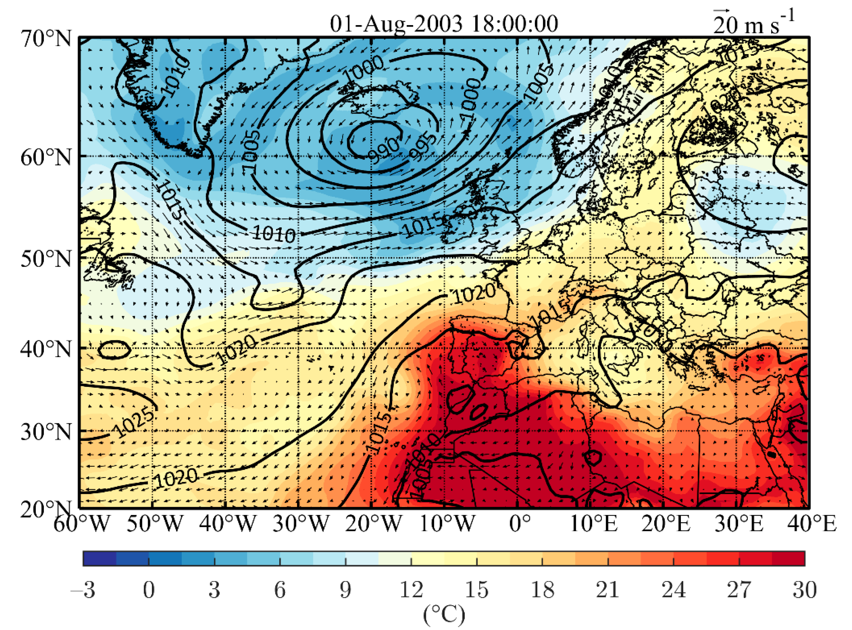
3.1. Synoptic Description of the Heatwave Event

Europe experienced extreme hot conditions during August 2003 which resulted in a persistent heatwave over the European continent [32]. For Portugal, a very strong heatwave developed between late July and early August. This heatwave was due to anticyclonic conditions with weak near-surface pressure gradients and a subtle low pressure southwest of the Iberian Peninsula which drove the weak, hot, and dry, near-surface southerly winds across the region (Figure 4). These conditions persisted from July 28th to August 2nd, and Portugal experienced record highest 850 hPa temperatures in August 1st and 2nd, since 1958 [65]. These conditions were in the origin of large forest fires [65] and an increase in mortality [66].

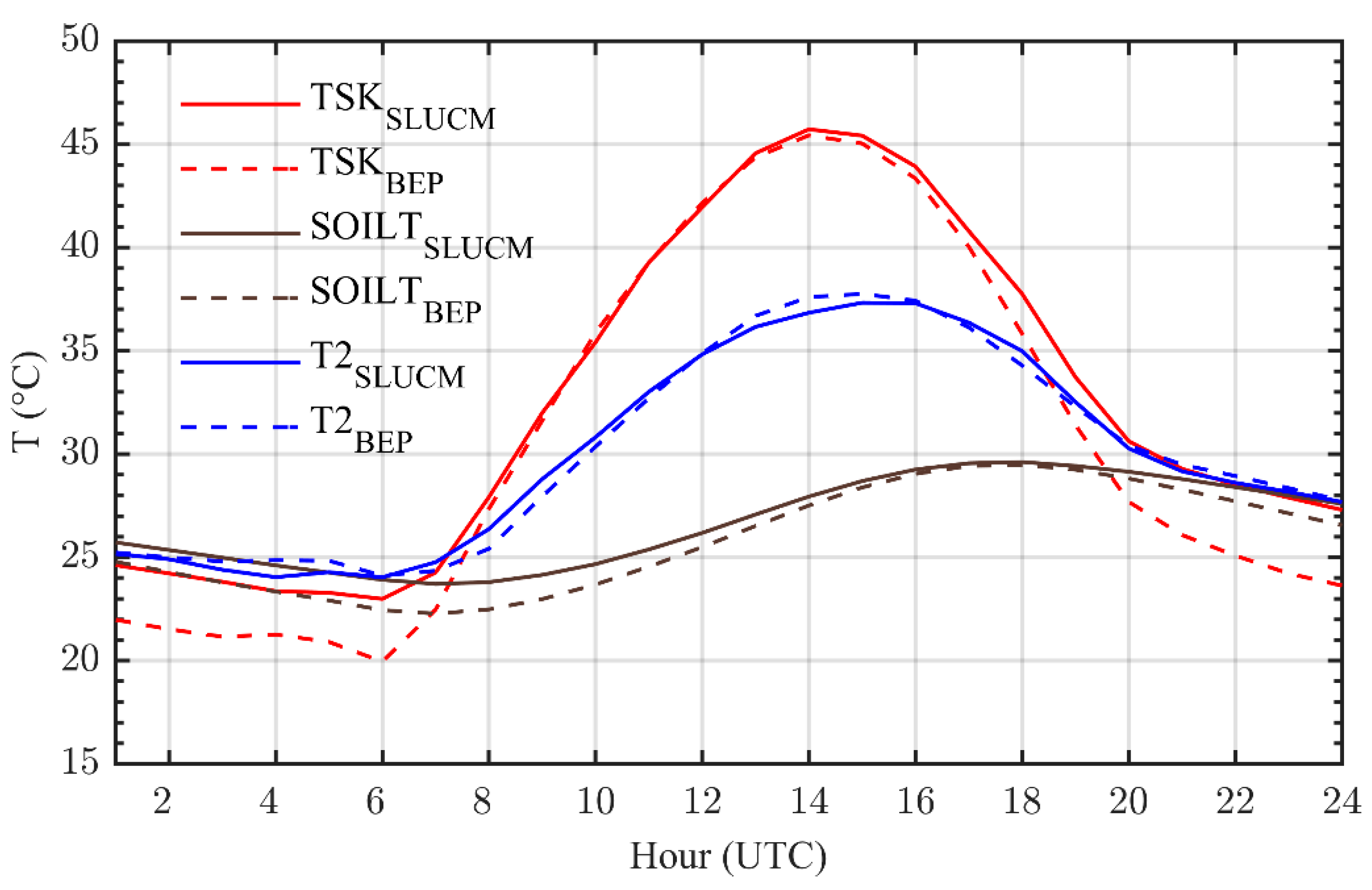
3.2. Model Evaluation

The evaluation of the modeled T2m was done by applying the formulations described in Section 2.2. A summary of the statistics and error measures between the observed and modeled T2m is shown in Table S2 of the Supplementary Material, for the nine meteorological stations of IPMA. According to Pielke (2013) [64], model skill is demonstrated when (1) STD_MOD ≈ STD_OBS, (2) RMSE < STD_OBS, and (3) RMSD < STD_OBS. These criteria are met for all the stations’ locations. Modeled minimum T2m is overestimated in SLUCM and BEP in almost every station location (on average 1.3 °C for SLUCM and 1.9 °C for BEP), but there is a significant improvement in these simulations compared with NO_SLUCM and NO_BEP, especially in SLUCM. In fact, SLUCM minimum temperature matches the observed values at Amadora and Cacém. Maximum temperature is underestimated in all simulations and locations (on average −3.3 °C for SLUCM and 2.9 °C for BEP), while the modeling of the mean temperature is significantly improved in SLUCM and BEP compared with NO_SLUCM and NO_BEP, and matches the observed values in SLUCM. Consequently, the mean temperature BIAS is reduced in all stations except in Estefânia, and RMSE, RMSD, and STDE are reduced by 0.4 °C. Finally, the Pearson correlation increases on average by 0.04 in SLUCM and 0.03 in BEP with respect to their control simulations (i.e., NO_SLUCM and NO_BEP) that use the Noah bulk scheme parameterization for the representation of urban land use surfaces.

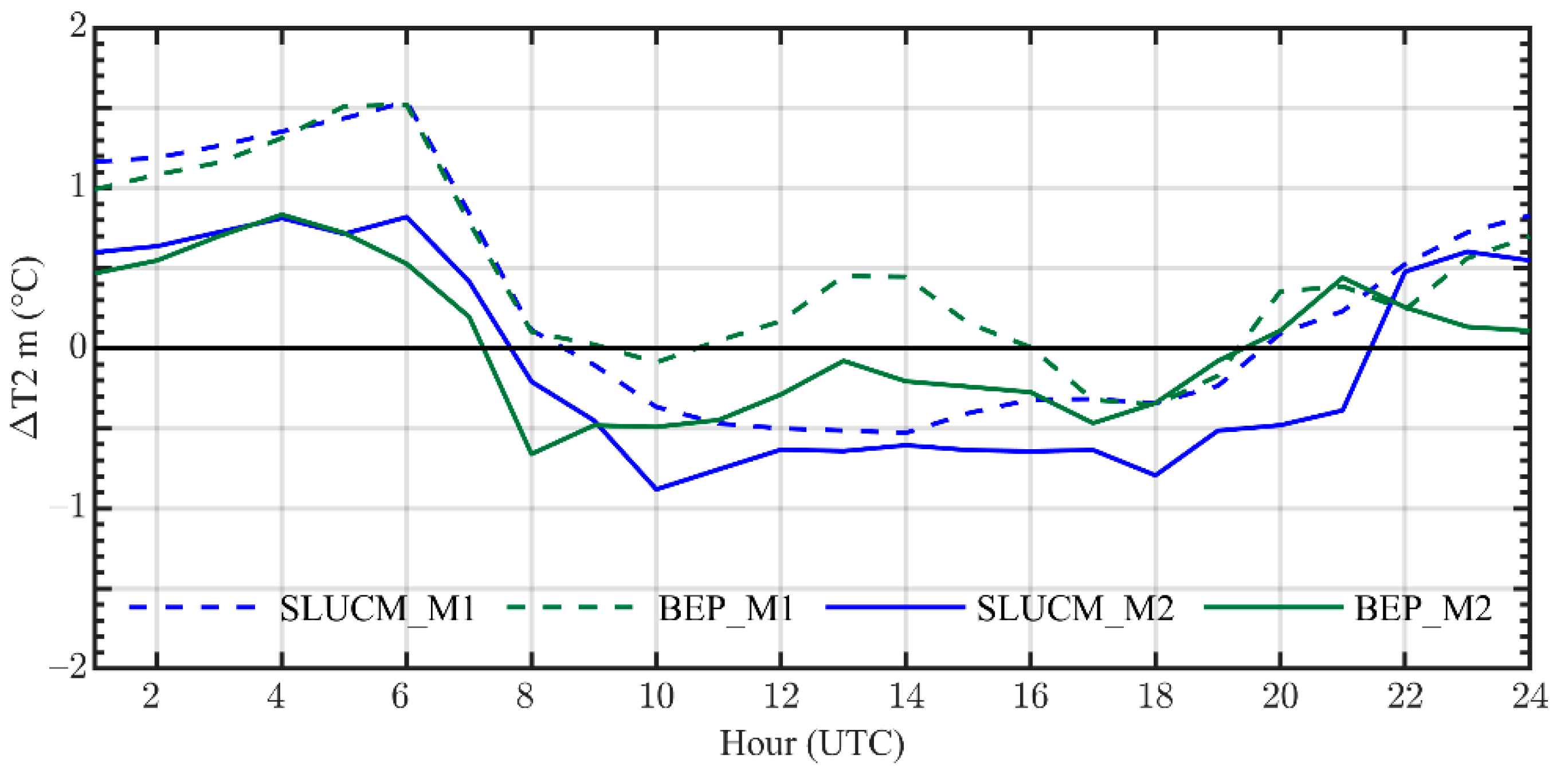
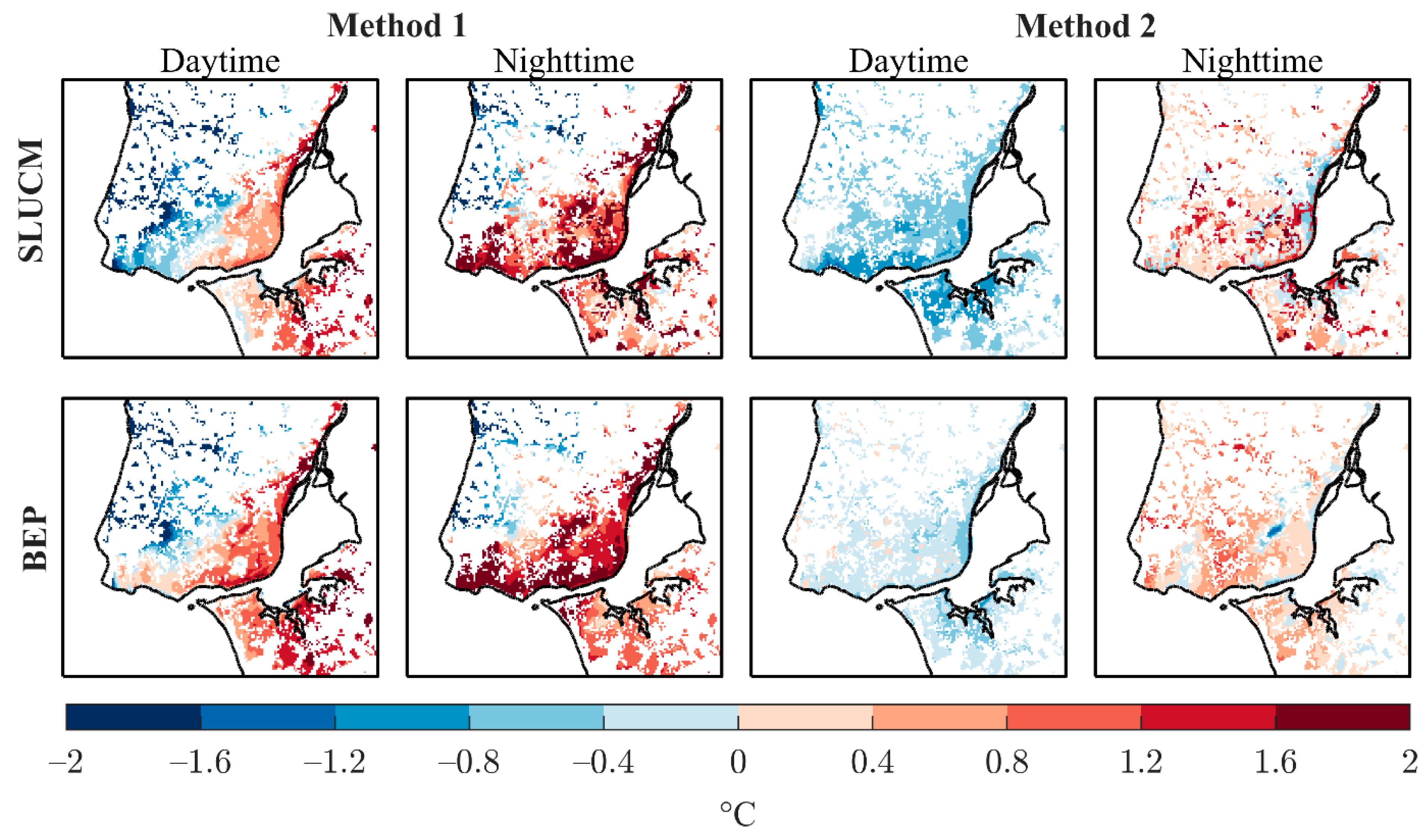
3.3. Urban Heat Island Analysis

In this subsection the modeled UHII and its spatial distribution is analyzed using the identification methods described in Section 2.3, namely the “classic method” and “local method”, hereafter called “Method 1” and “Method 2”, respectively.

Figure 5 shows the mean diurnal cycle of the Lisbon UHI during the heatwave period using SLUCM and BEP, and following the identification Method 1 and Method 2. The UHI diurnal profiles are quite different, with the application of Method 1 resulting in higher UHII throughout most of the night. As will be shown in Figure 6, the higher UHII using Method 1, for this particular heatwave, is related with the influence of the local geographic conditions that contribute to an exacerbation of the nighttime urban temperature due to the sheltering effect provided by the high topography present in the northern part of the domain, that blocks the prevailing north winds verified at the regional scale during most of the heatwave period (not shown). During the day, the UHII is much lower and negative in sign (i.e., UCI), except in BEP model using Method 1, which shows some fluctuations in the sign between positive and negative values. An ongoing research of the Lisbon UHI for future heatwaves resulting from different synoptic conditions shows that the occurrence of UCIs in the city is highly dependent on those conditions. Comparing the SLUCM and BEP UHIIs using Method 1, they are somewhat similar during the night, but very different during daytime, with SLUCM producing higher absolute values. Maximum near‑surface UHII values of around 1.5 ˚C and 0.8 ˚C are attained during the night using Method 1 and Method 2, respectively. The peak UHII is verified at around 0600 UTC for all methods and UCMs.

Regarding the contribution of the different urban classes to the UHI during nighttime, the HIR and the IC urban areas are the ones with the most influence (see Supplementary Material, Figure S1). A maximum UHII of 3.17 °C and 3.21 °C is attained during the nighttime in HIR and IC classes with SLUCM, respectively (1.93 °C and 1.95 °C in BEP). By using Method 2 and SLUCM, these values drop to 1.82 °C and 2.03 °C in HIR and IC classes (0.69 °C and 0.77 °C in BEP). Both nighttime maximum and mean values of UHII drop approximately 1 °C in HIR and IC classes when using BEP instead of SLUCM, regardless of the UHI identification method applied, while the UHII at night increases in LIR class when using BEP. During the day, an UCI is obtained in all urban classes by using Method 2, which means that during this period of the day the urban materials and features had an overall cooling effect.

Figure 6 shows the heatwave averaged daytime and nighttime near‑surface UHI fields obtained through Method 1 and Method 2 and using SLUCM and BEP UCMs. Both models show similar daytime averaged UHI patterns across the domain when using Method 1, with positive temperature anomalies at the north and south of the Tagus Estuary, and negative anomalies in the north-western part of the domain. In addition, the nighttime UHI pattern is similar to the daytime one. Both daytime and nighttime UHI fields exhibit the sheltering effect caused by the high topography in the north‑western part of the domain, which is manifested through the negative anomalies over this high topography region and by the positive anomalies at south. Hence, urban categories in the north-western part of the domain are much cooler than urban categories at south. This spatial behavior is consistent with what was found in previous studies of the Lisbon UHI [33,34,35,36,67]. However, the direct comparison with the results of those studies is limited, since they are focused on the evaluation of the UHI at the municipality scale and based on temperature anomalies for a very limited number of observational stations distributed within the municipality boundaries, while this study is done at the metropolitan scale and considers averages over all the urban/rural grid points. In the nighttime spatial patterns, SLUCM displays a greater contrast between the temperature anomalies of the different urban classes than BEP, despite the higher number of levels in BEP model’s configuration. Following Method 2, SLUCM and BEP UHI daytime patterns show negative temperature anomalies in most of the domain, that intensify closer to the Tagus Estuary. Larger negative values are obtained with SLUCM, meaning that replacing the urban fabric with Cropland and Woodland leads to higher T2m. Nighttime UHI values are positive in most of the domain but higher in SLUCM than in BEP, especially in the more densely occupied urban classes such as HIR and IC. During the heatwave period, the nighttime and daytime local-maximum instantaneous UHII can reach 6 ˚C for large areas when using Method 1 (not shown).

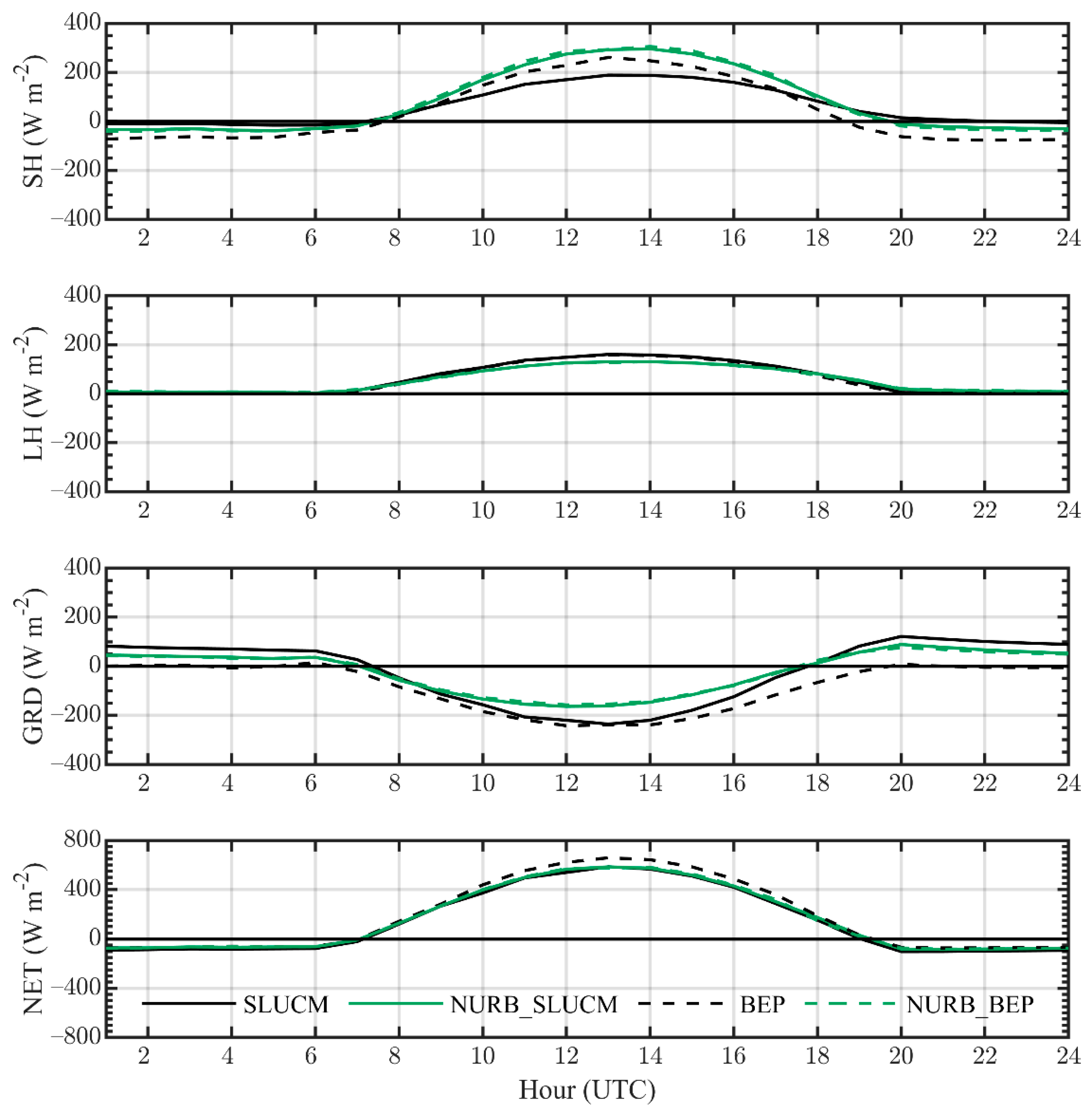
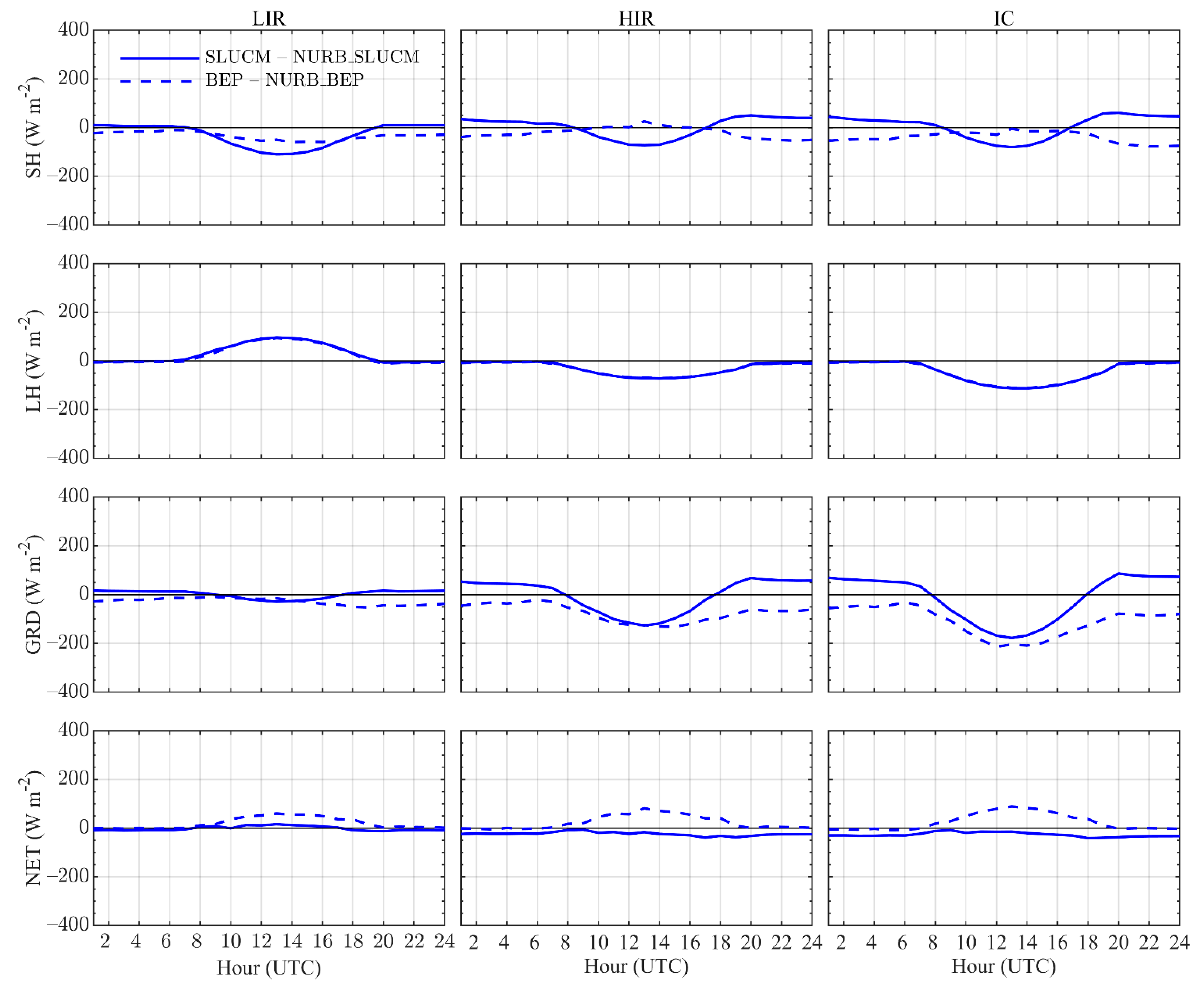
3.4. Surface Heat Fluxes

In this subsection, the causes of the differences in SLUCM and BEP simulations are analyzed. The balance between the incoming and outgoing components of the shortwave and longwave radiation at the surface can be translated in terms of the fluxes of SH, LH, and GRD [68]. As described in Section 2.1.2, in the WRF model these fluxes and the surface temperature at urban grid cells are estimated through the urban fraction parameter: the UCM computes the fluxes and surface temperature in the impervious fraction of the urban grid cells, while the land surface model (Noah LSM in this case) computes the fluxes and temperature in the vegetated fraction. The fluxes are direct outputs of the WRF model, with SH and LH heat fluxes being positive upward and GRD heat flux being positive downward. In the literature the GRD flux is also known as “storage heat flux”. In this study, the net balance (NET) of the fluxes is calculated as follows

$$\mathrm{NET}=\mathrm{HFX}+\mathrm{LH}-\mathrm{GRD}$$

(10)

Figure 7 shows the heatwave averaged mean diurnal cycle of the surface fluxes of SH, LH, GRD, and NET averaged over all the urban grid points. The fluxes are shown for SLUCM, BEP, NURB_SLUCM, and NURB_BEP simulations. No differences are found between NURB_SLUCM and NURB_BEP fluxes, which indicates that the different number of vertical levels in the simulations (46 and 49 levels, respectively) has no influence on the simulated fluxes. For this reason, any difference in the simulated fluxes of SLUCM and BEP simulations must be attributable to the different UCMs and to the way that they portray the urban canopy physical processes and features. Daytime SH and LH fluxes are positive in all simulations, while the GRD flux is negative as heat is being stored in the ground to be released into the atmosphere during nighttime. Peak values of surface heat fluxes are reached at around 1300 UTC which corresponds to the summer local noon. During nighttime, LH fluxes are negligible and SH fluxes are negative in most of the simulations (but very small in SLUCM), which means that the near-surface atmosphere is warmer than the surface. In contrast, GRD fluxes are positive in most simulations and small in BEP.

While most of the simulations agree in their daytime and nighttime heat fluxes signal, there are some unexpected differences between the simulations regarding the magnitude of the fluxes. For instance, NURB_SLUCM and NURB_BEP simulations have higher daytime SH flux values than SLUCM and BEP, indicating that during the day more SH is being released into the atmosphere when the urban fabric is removed and replaced with Cropland and Woodland. Furthermore, BEP simulation has a higher daytime SH flux than SLUCM, which has the lowest SH flux value of all the simulations. There is also an increase in the LH fluxes during the middle of the day in SLUCM and BEP, compared with NURB_SLUCM and NURB_BEP, which means that the presence of the urban land use classes leads to an increase of evapotranspiration. However, this increase is mainly associated with the LIR class that has 50% of green fraction as shown in Figure 8 and because LIR is the most represented urban class in terms of coverage area in the model domain. Nighttime GRD fluxes in BEP are very small and much lower than the other simulation experiments, especially compared with the SLUCM, despite the fact that the UHIIs are similar. As expected, during daytime, SLUCM and BEP simulations have larger negative values of GRD flux than NURB_SLUCM and NURB_BEP due to the smaller albedo and emissivity of the urban land use classes compared with Cropland and Woodland mosaic.

The net balance between all the fluxes shows that during the day surface fluxes are higher in simulations without urban fabric, which is in accordance with the diurnal near-surface UCI of Figure 5, obtained following Method 2. During the night, SLUCM has the higher (positive) values of total net flux and BEP the lower (negative) values. This translates into a difference of around 200 W m⁻² between SLUCM and BEP net fluxes during the night.

To further understand the impact of the urban fabric on the surface heat fluxes, Figure 8 shows the heatwave averaged decomposition of the differences between SLUCM and NURB_SLUCM and BEP and NURB_BEP simulations according to the three USGS33 urban classes (LIR, HIR, and IC). Consistent with what was found in Figure 7, the SH flux is reduced during the daytime in both SLUCM and BEP, when the urban classes are considered, but SLUCM simulations show a larger reduction compared to NURB_SLUCM (around 100 W m⁻² at 1300 UTC), especially in the LIR class. BEP has a smaller SH flux reduction during the day when compared with SLUCM, with LIR class showing the largest reduction. During the night, SLUCM shows an increase of around 50 W m⁻² in the SH fluxes for HIR and IC classes and a smaller increase for LIR. Conversely, BEP shows a reduction of SH fluxes in all urban classes, especially in the HIR and IC. The decomposition of the LH flux exhibits the same changes for SLUCM and BEP with respect to the NURB_SLUCM and NURB_BEP simulations. The HIR and IC classes contribute to the reduction of the LH fluxes, with the reduction reaching almost 100 W m⁻² in IC class during the peak of the day and slightly less in HIR. The LIR class contributes to an increase in LH fluxes of 100 W m⁻². Since LIR is the dominant class in the domain, the slight increase shown in the LH fluxes in Figure 7 for SLUCM and BEP simulations can be attributable to the LIR class. As expected, during the night the LH flux changes are very small in all urban classes. The downward GRD flux increases during the day mainly on the HIR and IC classes, and remains almost the same in the LIR class for both SLUCM and BEP. At night, the downward GRD flux increases in BEP simulation compared with NURB_BEP, meaning that heat is being transferred from the warmer atmosphere into the ground. Conversely, SLUCM shows an increase in the upward GRD flux. Lastly, there is a large reduction in the net radiation fluxes in HIR and IC classes during the day for both SLUCM and BEP, while LIR remains almost the same. At night, SLUCM shows an increase in net flux of around 100 W m⁻² in HIR and IC, but net fluxes remain unchanged in the LIR class. These fluxes are reduced in BEP simulation, but more in the HIR and IC classes.

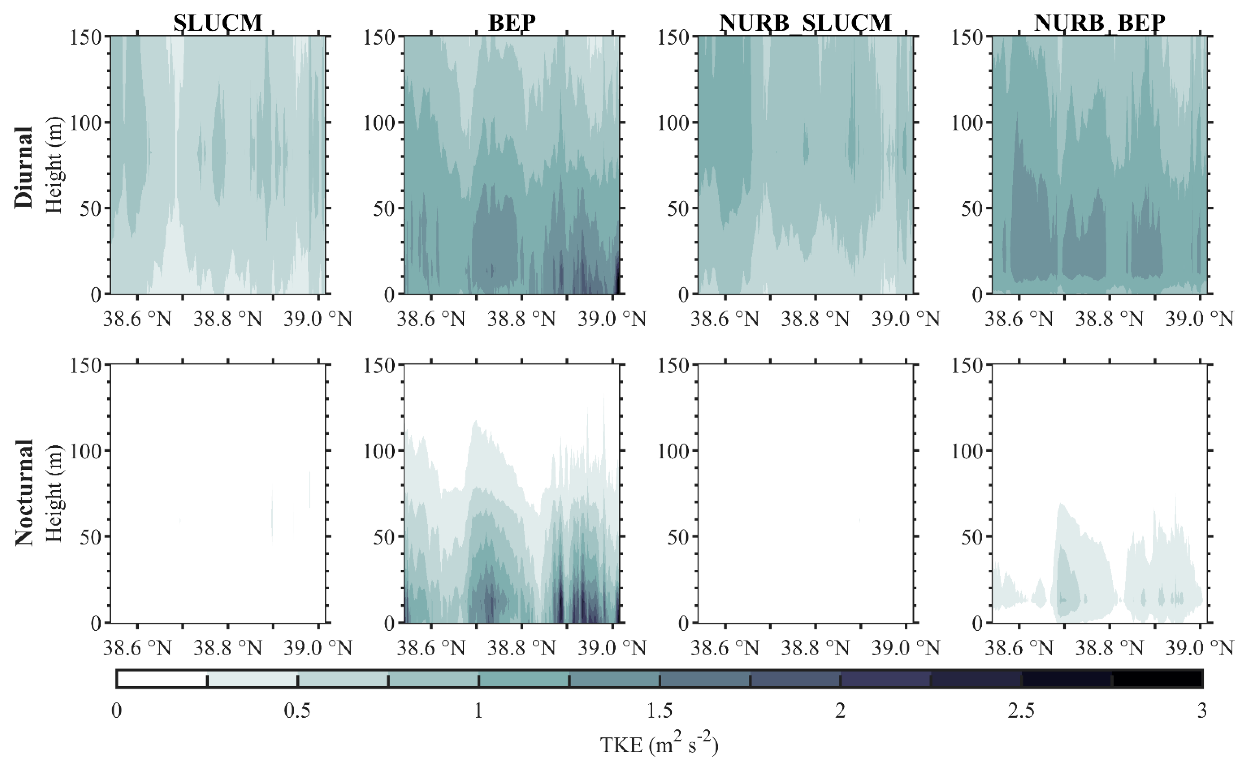
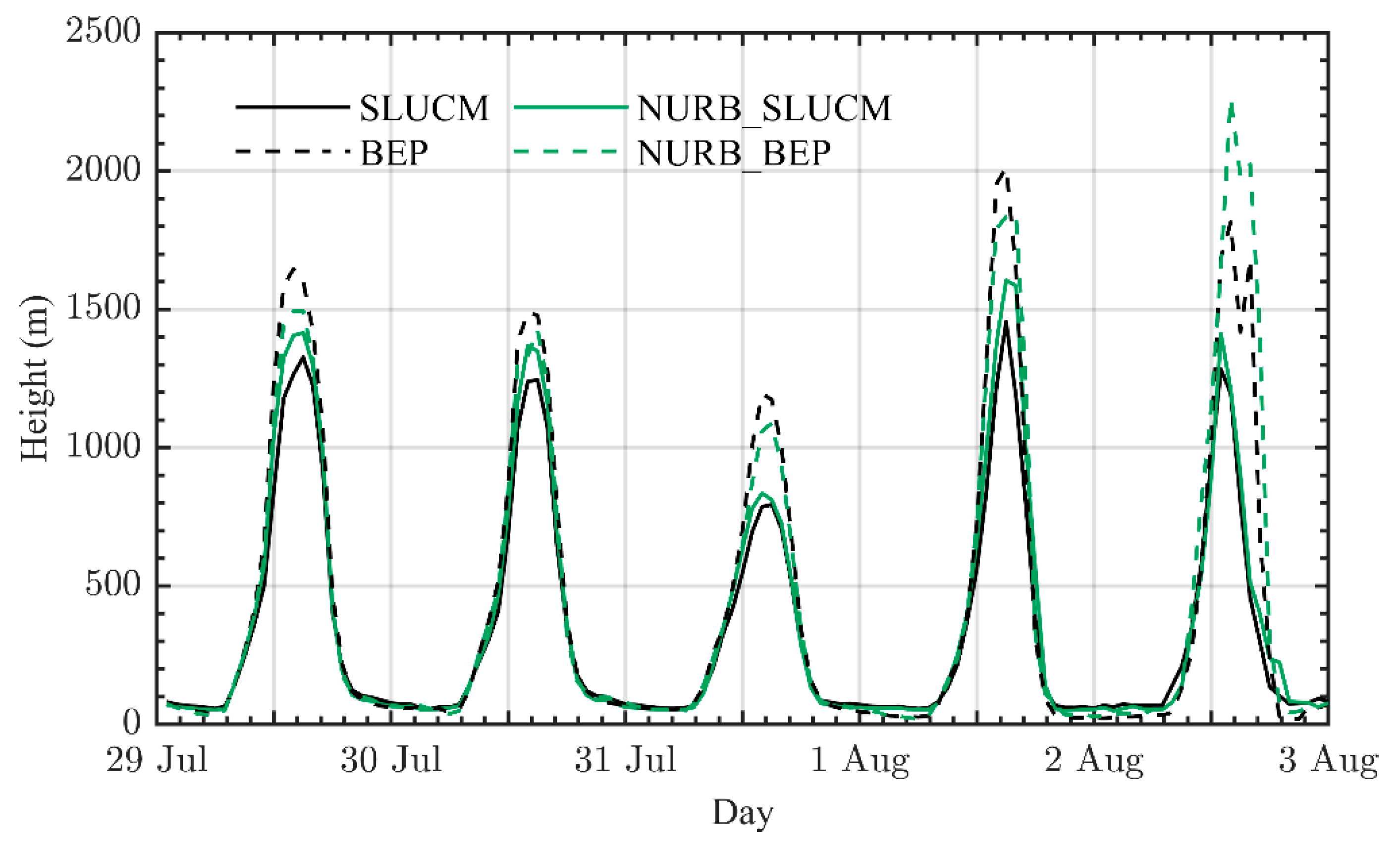
3.5. Vertical Analysis

Turbulent heat fluxes play a major role in the balance between surface and near-surface thermal properties. However, due to the low temporal frequency of the simulations output (60 min) it was not possible to compute the SH and LH turbulent fluxes. Instead, Figure 9 shows the heatwave averaged daytime and nighttime zonal means of TKE over urban grid points in the first 150 m of the PBL for SLUCM, NURB_SLUCM, BEP, and NURB_BEP simulations. SLUCM and NURB_SLUCM simulations produce smaller TKE values over urban locations than BEP and NURB_BEP during daytime, and very small TKE during nighttime. Additionally, nighttime values of TKE are much larger near the surface in BEP, dropping to very small values above ~100 m, although NURB_BEP has smaller TKE and only in the first 50 m of the PBL. This is due mainly to two reasons—the higher number of levels in the lower PBL in BEP and NURB_BEP simulations and to the different representation of the turbulent length scales in the TKE prognostic equation in BEP simulation, as this is the only UCM that directly parameterizes subgrid turbulent length scales within the urban canopy layer to account for the presence of buildings and that is specially designed to work with the BouLac PBL scheme [60,61]. Daytime TKE values in SLUCM and NURB_SLUCM are maximum at a height of ~90 m, which is ~36 m above the first model level in SLUCM/NURB_SLUCM simulations, while maximum values in BEP and NURB_BEP occur at ~20 m, which is ~8 m above the first model level in BEP/NURB_BEP simulations. Interestingly, the effect of the Tagus estuary on TKE is clearly visible a little lower than 38.7° N, where a decrease in TKE is seen in all simulations, especially during daytime. A similar behavior in TKE vertical structure was found for BEP and SLUCM by Teixeira et al. (2019) [69], which studied the Lisbon UHI surface to planetary boundary layer coupling during a heatwave event occurred between July 28 and August 22, 2010.

Through a retrospective analysis of the previous results, the high nighttime TKE values found for BEP in Figure 9 are possibly the main cause for its larger negative sensible heat fluxes shown in Figure 7 and for the lower near-surface UHII using Method 1 and Method 2 compared with SLUCM in HIR and IC classes. A possible mechanism that could explain these results is that larger turbulent sensible heat fluxes, associated with higher nighttime TKE values near the surface, promote rapid surface cooling and, hence, a greater thermal gradient between the surface and the lower atmosphere. To compensate for this rapid surface cooling, the heat accumulated in the ground during daytime and later converted into SH at the surface (at night), is immediately transported by the turbulent fluxes. This feedback mechanism can be clearly seen through the lower rate of change of GRD flux in BEP simulation between 1400 UTC and 2000 UTC (Figure 7) when comparing SLUCM, NURB_SLUCM, and NURB_BEP simulations.

Supporting the existence of such mechanism, Figure 10 shows the heatwave averaged mean diurnal cycle of surface skin temperature (TSK), first layer soil temperature (SOILT), and T2m, averaged over urban grid points. Despite having similar T2m values to SLUCM and sometimes even higher, on average TSK in BEP is 3 °C lower and 2 °C lower soil temperature than SLUCM during the nighttime period. However, during nighttime $\mathrm{T}{2}_{\mathrm{BEP}}>{\mathrm{SOILT}}_{\mathrm{BEP}}>{\mathrm{TSK}}_{\mathrm{BEP}}$, which together with the higher TKE close to the surface could explain the negative SH flux and the very small GRD flux shown in BEP simulation during nighttime.

Following the TKE analysis, Figure 11 shows the comparison between the modeled planetary boundary layer height (PBLH) time series of SLUCM, BEP, NURB_SLUCM, and NURB_BEP during the heatwave period. In WRF, the BouLac PBL scheme is responsible for the diagnostic of PBLH, which is defined within the scheme as the height where the prognostic TKE reduces to a value of 0.005 m² s⁻². As expected, the PBLH rapidly responds to surface forcings, as shown by its diurnal cycle where lower PBLH values are seen during nighttime and maximum values at local noon. The daytime maximums of PBLH decrease in the first three days of the heatwave period and increase afterwards, except for SLUCM and NURB_SLUCM simulations. Maximum absolute values are seen on August 1st for SLUCM (~1800 m) and NURB_SLUCM (~2300 m) and on August 2nd for BEP (~1400 m) and NURB_BEP (~1600 m). The PBLH during the middle of the day is always higher for simulations with larger number of vertical levels, especially for BEP simulation, except on August 2nd when NURB_BEP predicts higher PBLH. Interestingly, NURB_BEP predicts the highest PBLH of all the simulations on August 2, but in the previous days the PBLH is higher in BEP, which means that according to BEP, the inclusion of the urban classes contributes to an increase of the PBLH during the early afternoon. Contrarily to BEP, SLUCM predicts the lowest PBLH despite the higher roughness length of the urban classes.

Lastly, the modeled PBLH at 1200 UTC was compared with observations collected from soundings at the Lisbon Airport meteorological station during the entire heatwave period (Supplementary Material, Figure S2). To estimate the PBLH from the sounding profiles, a “simple parcel method” [70] was used, which defines the PBLH as the height at which virtual potential temperature equals its surface value. The results show that SLUCM consistently diagnoses better the PBLH than BEP and almost matches the sounding PBLH on July 29 and August 1 at 1200 UTC. BEP significantly overestimates PBLH, especially on July 29 and 30, which may be a consequence of its higher daytime TKE values. However, in all days, the mixed layer is still slightly stable and, therefore, not fully mixed. These results contrast with the ones obtained for the PBL height in Teixeira et al. (2019) [69] study, which uses only one model level within the urban canopy layer in BEP simulations. This shows that BEP model simulations results are highly sensitive to the number and vertical distribution of model levels within the urban canopy layer. Thus, UHI studies using BEP model should include a sensitivity analysis to the number and vertical distribution of the model levels within the urban canopy.

4. Conclusions

This work compared the performance and respective interactions of two UCMs and UHI identification methods during the record‑breaking August 2003 heatwave, in the city of Lisbon, Portugal. To this end, the WRF model was coupled with SLUCM and BEP UCMs, and two distinct UHI identification methods were used, namely, the “classic method” (Method 1) and “local method” (Method 2).

Results reveal significant improvements in modeled minimum and mean T2m when using WRF coupled with the UCMs, albeit SLUCM better predicts minimum and mean temperature and BEP maximum temperature. The domain averaged UHII using both identification methods revealed the existence of a nighttime UHI and a daytime UCI when using SLUCM or BEP, except for Method 1 using BEP. The domain averaged UHII for SLUCM and BEP is similar during nighttime, but very different during the day, with SLUCM producing higher UHII absolute values. Maximum near-surface UHII of around 1.5 °C and 0.8 °C are attained during the night using Method 1 and Method 2, respectively, with the application of Method 1 always resulting in higher UHII than Method 2. However, the analysis of the UHI spatial patterns using Method 1 revealed that the local geography has a great influence on the UHII and distribution at the metropolitan scale, due to the sheltering effect of the high topography in the north-western part of the domain, that blocks the prevailing northern winds during the heatwave and inhibits the advective cooling in the south-eastern part of the city’s metropolitan area. This effect contributes to the intensification of the UHI at the south of the high topography region and to the reduction over it, despite this dipole signal being much stronger during nighttime than during daytime. The spatial patterns using Method 2 during daytime and nighttime show an overall urban cooling effect and an overall urban warming effect across the whole domain, respectively. This spatial behavior due to the influence of the high northern topography sheltering effect is consistent with what was found in previous studies of the Lisbon UHI occurring under prevailing northern wind conditions [33,34,35,36,67].

The surface heat fluxes at urban locations revealed that the urban classes contribute for the reduction of the SH fluxes during the day compared with the case where the urban classes are replaced with natural vegetation, even if the reduction in BEP is greater. At night, SH fluxes are extremely small in SLUCM and negative in BEP, meaning that heat is being transferred from the atmosphere into the surface. The LH release also increases for both UCMs during the middle of the day when the urban fabric is considered, due to the larger green fraction of LIR class. Conversely, HIR and IC classes contribute to the reduction of the LH fluxes. GRD fluxes increase in SLUCM and decrease in BEP in comparison with simulations where the urban classes were replaced by natural vegetation. The analysis of TKE zonal averages in the first meters of the PBL at urban grid points locations shows that BEP produces large TKE values close to the surface during the night, while SLUCM TKE values are very small. This may be the cause of the negative SH fluxes and lower near‑surface UHII found in BEP during the night in HIR and IC classes. A closer look at the diurnal cycle profiles of SOILT, TSK, and T2m over urban grid points supports the idea that the larger negative SH fluxes found in BEP, associated with higher nocturnal TKE values near the surface, promote a rapid surface cooling and consequently a greater thermal gradient between the surface and the lower atmosphere. To compensate for this rapid surface cooling, the heat accumulated in the ground during the day and later converted into SH at the surface (at night), is immediately transported by the turbulent fluxes. As a result of its higher TKE, BEP predicts higher PBLH than SLUCM. Comparing the simulated PBLH with observed values derived from 1200 UTC soundings at Gago Coutinho station shows both SLUCM and BEP overestimate PBLH, but this overestimation is much larger in BEP.

Given the results and conclusions here presented, the importance and advantage of using WRF coupled with UCMs to study UHIs becomes clear. Although SLUCM model performed better than BEP for this particular heatwave and model setup, a previous study using a similar model configuration, but with only one level within the urban canopy for BEP (compared with three in this study), shows opposite results. Hence, UHI modeling studies using BEP should consider a sensitivity test to the number and distribution of vertical levels. Regarding the UHI identification methods, the use of both classic and local methods is important to differentiate the geographic and urban canopy contributions to UHIs, but since the ultimate goal of UHI studies is to develop UHI mitigation measures, the use of the “local method” (Method 2) is the best option. However, this method may present limitations in its application to other cities, regarding the type of land use that replaces the urban fabric. This is especially true for cities with more heterogeneous natural land use.

References

1. Oke, T. City Size and the Urban Heat Island. Atmos. Environ. 1973, 7, 769–779. [Google Scholar] [CrossRef]
2. Dong, L.; Mitra, C.; Greer, S.; Burt, E. The Dynamical Linkage of Atmospheric Blocking to Drought, Heatwave and Urban Heat Island in Southeastern US: A Multi-Scale Case Study. Atmosphere 2018, 9, 33. [Google Scholar] [CrossRef] [Green Version]
3. Rasul, A.; Balzter, H.; Smith, C.; Remedios, J.; Adamu, B.; Sobrino, J.; Srivanit, M.; Weng, Q. A Review on Remote Sensing of Urban Heat and Cool Islands. Land 2017, 6, 38. [Google Scholar] [CrossRef] [Green Version]
4. Rizwan, A.M.; Dennis, L.Y.C.; Liu, C. A Review on the Generation, Determination and Mitigation of Urban Heat Island. J. Environ. Sci. 2008, 20, 120–128. [Google Scholar] [CrossRef]
5. Markowski, P.; Richardson, Y. Mesoscale Meteorology in Midlatitudes; John Wiley & Sons, Ltd.: Chichester, UK, 2010; ISBN 978-0-470-68210-4. [Google Scholar]
6. Oke, T.R. Canyon Geometry and the Nocturnal Urban Heat Island: Comparison of Scale Model and Field Observations. J. Climatol. 1981, 1, 237–254. [Google Scholar] [CrossRef]
7. Arnfield, A.J. Two Decades of Urban Climate Research: A Review of Turbulence, Exchanges of Energy and Water, and the Urban Heat Island. Int. J. Climatol. 2003, 23, 1–26. [Google Scholar] [CrossRef]
8. Unger, J. Intra-Urban Relationship between Surface Geometry and Urban Heat Island: Review and New Approach. Clim. Res. 2004, 27, 253–264. [Google Scholar] [CrossRef] [Green Version]
9. Morini, E.; Touchaei, A.; Castellani, B.; Rossi, F.; Cotana, F. The Impact of Albedo Increase to Mitigate the Urban Heat Island in Terni (Italy) Using the WRF Model. Sustainability 2016, 8, 999. [Google Scholar] [CrossRef] [Green Version]
10. Weng, Q.; Lu, D.; Schubring, J. Estimation of Land Surface Temperature–Vegetation Abundance Relationship for Urban Heat Island Studies. Remote Sens. Environ. 2004, 89, 467–483. [Google Scholar] [CrossRef]
11. Wong, N.H.; Yu, C. Study of Green Areas and Urban Heat Island in a Tropical City. Habitat Int. 2005, 29, 547–558. [Google Scholar] [CrossRef]
12. Feng, J.-M.; Wang, Y.-L.; Ma, Z.-G.; Liu, Y.-H. Simulating the Regional Impacts of Urbanization and Anthropogenic Heat Release on Climate across China. J. Clim. 2012, 25, 7187–7203. [Google Scholar] [CrossRef]
13. Ziter, C.D.; Pedersen, E.J.; Kucharik, C.J.; Turner, M.G. Scale-Dependent Interactions between Tree Canopy Cover and Impervious Surfaces Reduce Daytime Urban Heat during Summer. Proc. Natl. Acad. Sci. USA 2019, 116, 7575–7580. [Google Scholar] [CrossRef] [Green Version]
14. Nastran, M.; Kobal, M.; Eler, K. Urban Heat Islands in Relation to Green Land Use in European Cities. Urban For. Urban Green. 2019, 37, 33–41. [Google Scholar] [CrossRef] [Green Version]
15. Li, D.; Liao, W.; Rigden, A.J.; Liu, X.; Wang, D.; Malyshev, S.; Shevliakova, E. Urban Heat Island: Aerodynamics or Imperviousness? Sci. Adv. 2019, 5, eaau4299. [Google Scholar] [CrossRef] [PubMed] [Green Version]
16. Manoli, G.; Fatichi, S.; Schläpfer, M.; Yu, K.; Crowther, T.W.; Meili, N.; Burlando, P.; Katul, G.G.; Bou-Zeid, E. Magnitude of Urban Heat Islands Largely Explained by Climate and Population. Nature 2019, 573, 55–60. [Google Scholar] [CrossRef]
17. Shahmohamadi, P.; Che-Ani, A.I.; Maulud, K.N.A.; Tawil, N.M.; Abdullah, N.A.G. The Impact of Anthropogenic Heat on Formation of Urban Heat Island and Energy Consumption Balance. Urban Stud. Res. 2011, 2011, 1–9. [Google Scholar] [CrossRef] [Green Version]
18. Salamanca, F.; Georgescu, M.; Mahalov, A.; Moustaoui, M.; Wang, M. Anthropogenic Heating of the Urban Environment Due to Air Conditioning: Anthropogenic Heating Due to AC. J. Geophys. Res. Atmos. 2014, 119, 5949–5965. [Google Scholar] [CrossRef]
19. Sailor, D.J.; Georgescu, M.; Milne, J.M.; Hart, M.A. Development of a National Anthropogenic Heating Database with an Extrapolation for International Cities. Atmos. Environ. 2015, 118, 7–18. [Google Scholar] [CrossRef] [Green Version]
20. Stewart, I.D. A Systematic Review and Scientific Critique of Methodology in Modern Urban Heat Island Literature. Int. J. Climatol. 2011, 31, 200–217. [Google Scholar] [CrossRef]
21. Lowry, W.P. Empirical Estimation of Urban Effects on Climate: A Problem Analysis. J. Appl. Meteorol. 1977, 16, 129–135. [Google Scholar] [CrossRef] [Green Version]
22. Georgescu, M.; Moustaoui, M.; Mahalov, A.; Dudhia, J. An Alternative Explanation of the Semiarid Urban Area “Oasis Effect”: The Semiarid Urban Area “Oasis Effect”. J. Geophys. Res. Atmos. 2011, 116. [Google Scholar] [CrossRef]
23. Ma, S.; Pitman, A.; Hart, M.; Evans, J.P.; Haghdadi, N.; MacGill, I. The Impact of an Urban Canopy and Anthropogenic Heat Fluxes on Sydney’s Climate. Int. J. Climatol. 2017, 37, 255–270. [Google Scholar] [CrossRef]
24. Li, D.; Bou-Zeid, E. Synergistic Interactions between Urban Heat Islands and Heat Waves: The Impact in Cities Is Larger than the Sum of Its Parts. J. Appl. Meteorol. Climatol. 2013, 52, 2051–2064. [Google Scholar] [CrossRef] [Green Version]
25. Ramamurthy, P.; González, J.; Ortiz, L.; Arend, M.; Moshary, F. Impact of Heatwave on a Megacity: An Observational Analysis of New York City during July 2016. Environ. Res. Lett. 2017, 12, 054011. [Google Scholar] [CrossRef]
26. Rogers, C.D.W.; Gallant, A.J.E.; Tapper, N.J. Is the Urban Heat Island Exacerbated during Heatwaves in Southern Australian Cities? Theor. Appl. Climatol. 2019, 137, 441–457. [Google Scholar] [CrossRef]
27. Heaviside, C.; Macintyre, H.; Vardoulakis, S. The Urban Heat Island: Implications for Health in a Changing Environment. Curr. Environ. Health Rep. 2017, 4, 296–305. [Google Scholar] [CrossRef] [PubMed]
28. IPCC Climate Change 2013: The Physical Science Basis. Contribution of Working Group I to the Fifth Assessment Report of the Intergovernmental Panel on Climate Change 2013; IPCC: Geneva, Switzerland, 2013.
29. Rocha, A.; Pereira, S.C.; Viceto, C.; Silva, R.; Neto, J.; Marta-Almeida, M. A Consistent Methodology to Evaluate Temperature and Heat Wave Future Projections for Cities: A Case Study for Lisbon. Appl. Sci. 2020, 10, 1149. [Google Scholar] [CrossRef] [Green Version]
30. Jacob, D.; Petersen, J.; Eggert, B.; Alias, A.; Christensen, O.B.; Bouwer, L.M.; Braun, A.; Colette, A.; Déqué, M.; Georgievski, G.; et al. EURO-CORDEX: New High-Resolution Climate Change Projections for European Impact Research. Reg. Environ. Chang. 2014, 14, 563–578. [Google Scholar] [CrossRef]
31. Schär, C.; Vidale, P.L.; Lüthi, D.; Frei, C.; Häberli, C.; Liniger, M.A.; Appenzeller, C. The Role of Increasing Temperature Variability in European Summer Heatwaves. Nature 2004, 427, 332–336. [Google Scholar] [CrossRef]
32. García-Herrera, R.; Díaz, J.; Trigo, R.M.; Luterbacher, J.; Fischer, E.M. A Review of the European Summer Heat Wave of 2003. Crit. Rev. Environ. Sci. Technol. 2010, 40, 267–306. [Google Scholar] [CrossRef]
33. Alcoforado, M.-J.; Andrade, H. Nocturnal Urban Heat Island in Lisbon (Portugal): Main Features and Modelling Attempts. Theor. Appl. Climatol. 2006, 84, 151–159. [Google Scholar] [CrossRef]
34. Lopes, A.; Alves, E.; Alcoforado, M.J.; Machete, R. Lisbon Urban Heat Island Updated: New Highlights about the Relationships between Thermal Patterns and Wind Regimes. Adv. Meteorol. 2013, 2013, 1–11. [Google Scholar] [CrossRef]
35. Alcoforado, M.-J.; Lopes, A.; Alves, E.; Canário, P. Lisbon’s Urban Heat Island. Statistical Study 2004–2012. Finisterra 2014, 48, 61–80. [Google Scholar] [CrossRef] [Green Version]
36. Oliveira, A.; Lopes, A.; Correia, E.; Niza, S.; Soares, A. Heatwaves and Summer Urban Heat Islands: A Daily Cycle Approach to Unveil the Urban Thermal Signal Changes in Lisbon, Portugal. Atmosphere 2021, 12, 292. [Google Scholar] [CrossRef]
37. Skamarock, W.; Klemp, J.; Dudhia, J.; Gill, D.; Barker, D.; Duda, M.; Huang, X.-Y.; Wang, W.; Powers, J. A Description of the Advanced Research WRF Version 3; University Corporation for Atmospheric Research: Boulder, CO, USA, 2008. [Google Scholar]
38. Powers, J.G.; Klemp, J.B.; Skamarock, W.C.; Davis, C.A.; Dudhia, J.; Gill, D.O.; Coen, J.L.; Gochis, D.J.; Ahmadov, R.; Peckham, S.E.; et al. The Weather Research and Forecasting Model: Overview, System Efforts, and Future Directions. Bull. Am. Meteorol. Soc. 2017, 98, 1717–1737. [Google Scholar] [CrossRef]
39. Dee, D.P.; Uppala, S.M.; Simmons, A.J.; Berrisford, P.; Poli, P.; Kobayashi, S.; Andrae, U.; Balmaseda, M.A.; Balsamo, G.; Bauer, P.; et al. The ERA-Interim Reanalysis: Configuration and Performance of the Data Assimilation System. Q. J. R. Meteorol. Soc. 2011, 137, 553–597. [Google Scholar] [CrossRef]
40. Marta-Almeida, M.; Teixeira, J.C.; Carvalho, M.J.; Melo-Gonçalves, P.; Rocha, A.M. High Resolution WRF Climatic Simulations for the Iberian Peninsula: Model Validation. Phys. Chem. Earth Parts ABC 2016, 94, 94–105. [Google Scholar] [CrossRef]
41. Miguez-Macho, G.; Stenchikov, G.L.; Robock, A. Spectral Nudging to Eliminate the Effects of Domain Position and Geometry in Regional Climate Model Simulations. J. Geophys. Res. Atmos. 2004, 109. [Google Scholar] [CrossRef] [Green Version]
42. Jacobs, S.J.; Gallant, A.J.E.; Tapper, N.J. The Sensitivity of Urban Meteorology to Soil Moisture Boundary Conditions: A Case Study in Melbourne, Australia. J. Appl. Meteorol. Climatol. 2017, 56, 2155–2172. [Google Scholar] [CrossRef]
43. Xue, H.; Jin, Q.; Yi, B.; Mullendore, G.L.; Zheng, X.; Jin, H. Modulation of Soil Initial State on WRF Model Performance Over China. J. Geophys. Res. Atmos. 2017, 122, 11278–11300. [Google Scholar] [CrossRef]
44. Li, M.; Wu, P.; Ma, Z. A Comprehensive Evaluation of Soil Moisture and Soil Temperature from Third-Generation Atmospheric and Land Reanalysis Data Sets. Int. J. Climatol. 2020, 40, 5744–5766. [Google Scholar] [CrossRef]
45. Hong, S.-Y.; Lim, J.-O.J. The WRF Single-Moment 6-Class Microphysics Scheme (WSM6). Asia-Pac. J. Atmos. Sci. 2006, 42, 129–151. [Google Scholar]
46. Dudhia, J. Numerical Study of Convection Observed during the Winter Monsoon Experiment Using a Mesoscale Two-Dimensional Model. J. Atmos. Sci. J Atmos. Sci. 1989, 46, 3077–3107. [Google Scholar] [CrossRef]
47. Mlawer, E.J.; Taubman, S.J.; Brown, P.D.; Iacono, M.J.; Clough, S.A. Radiative Transfer for Inhomogeneous Atmospheres: RRTM, a Validated Correlated-k Model for the Longwave. J. Geophys. Res. Atmos. 1997, 102, 16663–16682. [Google Scholar] [CrossRef] [Green Version]
48. Jiménez, P.A.; Dudhia, J.; González-Rouco, J.F.; Navarro, J.; Montávez, J.P.; García-Bustamante, E. A Revised Scheme for the WRF Surface Layer Formulation. Mon. Weather Rev. 2011, 140, 898–918. [Google Scholar] [CrossRef] [Green Version]
49. Bougeault, P.; Lacarrere, P. Parameterization of Orography-Induced Turbulence in a Mesobeta—Scale Model. Mon. Weather Rev. 1989, 117, 1872–1890. [Google Scholar] [CrossRef]
50. Chen, F.; Dudhia, J. Coupling an Advanced Land Surface–Hydrology Model with the Penn State–NCAR MM5 Modeling System. Part I: Model Implementation and Sensitivity. Mon. Weather Rev. 2001, 129, 569–585. [Google Scholar] [CrossRef] [Green Version]
51. Grell, G.A.; Freitas, S.R. A Scale and Aerosol Aware Stochastic Convective Parameterization for Weather and Air Quality Modeling. Atmos. Chem. Phys. 2014, 14, 5233–5250. [Google Scholar] [CrossRef] [Green Version]
52. Farr, T.; Rosen, P.; Caro, E.; Crippen, R.; Duren, R.; Hensley, S.; Kobrick, M.; Paller, M.; Rodriguez, E.; Roth, L.; et al. The Shuttle Radar Topography Mission. Rev. Geophys 2007, 45. [Google Scholar] [CrossRef] [Green Version]
53. Büttner, G. CORINE Land Cover and Land Cover Change Products. In Land Use and Land Cover Mapping in Europe: Practices & Trends; Manakos, I., Braun, M., Eds.; Springer: Dordrecht, The Netherlands, 2014; pp. 55–74. ISBN 978-94-007-7969-3. [Google Scholar]
54. Pineda, N.; Jorba, O.; Jorge, J.; Baldasano, J.M. Using NOAA AVHRR and SPOT VGT Data to Estimate Surface Parameters: Application to a Mesoscale Meteorological Model. Int. J. Remote Sens. 2004, 25, 129–143. [Google Scholar] [CrossRef]
55. Carvalho, D.; Martins, H.; Marta-Almeida, M.; Rocha, A.; Borrego, C. Urban Resilience to Future Urban Heat Waves under a Climate Change Scenario: A Case Study for Porto Urban Area (Portugal). Urban Clim. 2017, 19, 1–27. [Google Scholar] [CrossRef]
56. Stewart, I.D.; Oke, T.R. Local Climate Zones for Urban Temperature Studies. Bull. Am. Meteorol. Soc. 2012, 93, 1879–1900. [Google Scholar] [CrossRef]
57. Oliveira, A.; Lopes, A.; Niza, S. Local Climate Zones in Five Southern European Cities: An Improved GIS-Based Classification Method Based on Copernicus Data. Urban Clim. 2020, 33, 100631. [Google Scholar] [CrossRef]
58. Kusaka, H.; Kondo, H.; Kikegawa, Y.; Kimura, F. A Simple Single-Layer Urban Canopy Model For Atmospheric Models: Comparison With Multi-Layer And Slab Models. Bound. Layer Meteorol. 2001, 101, 329–358. [Google Scholar] [CrossRef]
59. Kusaka, H.; KIMURA, F. Coupling a Single-Layer Urban Canopy Model with a Simple Atmospheric Model: Impact on Urban Heat Island Simulation for an Idealized Case. J. Meteorol. Soc. Jpn. 2004, 82, 67–80. [Google Scholar] [CrossRef] [Green Version]
60. Martilli, A.; Clappier, A.; Rotach, M.W. An Urban Surface Exchange Parameterisation for Mesoscale Models. Bound. Layer Meteorol. 2002, 104, 261–304. [Google Scholar] [CrossRef]
61. Chen, F.; Kusaka, H.; Bornstein, R.; Ching, J.; Grimmond, C.S.B.; Grossman-Clarke, S.; Loridan, T.; Manning, K.W.; Martilli, A.; Miao, S.; et al. The Integrated WRF/Urban Modelling System: Development, Evaluation, and Applications to Urban Environmental Problems. Int. J. Climatol. 2011, 31, 273–288. [Google Scholar] [CrossRef]
62. Yang, J.; Wang, Z.-H.; Chen, F.; Miao, S.; Tewari, M.; Voogt, J.A.; Myint, S. Enhancing Hydrologic Modelling in the Coupled Weather Research and Forecasting–Urban Modelling System. Bound. Layer Meteorol. 2015, 155, 87–109. [Google Scholar] [CrossRef]
63. Keyser, D.; Anthes, R.A. The Applicability of a Mixed–Layer Model of the Planetary Boundary Layer to Real-Data Forecasting. Mon. Weather Rev. 1977, 105, 1351–1371. [Google Scholar] [CrossRef] [Green Version]
64. Pielke, R.A. Mesoscale Meteorological Modeling; Elsevier Science: Amsterdam, The Netherlands, 2013; ISBN 978-0-12-385238-0. [Google Scholar]
65. Trigo, R.M.; Pereira, J.M.C.; Pereira, M.G.; Mota, B.; Calado, T.J.; Dacamara, C.C.; Santo, F.E. Atmospheric Conditions Associated with the Exceptional Fire Season of 2003 in Portugal. Int. J. Climatol. 2006, 26, 1741–1757. [Google Scholar] [CrossRef]
66. Trigo, R.M.; Ramos, A.M.; Nogueira, P.J.; Santos, F.D.; Garcia-Herrera, R.; Gouveia, C.; Santo, F.E. Evaluating the Impact of Extreme Temperature Based Indices in the 2003 Heatwave Excessive Mortality in Portugal. Environ. Sci. Policy 2009, 12, 844–854. [Google Scholar] [CrossRef]
67. Alcoforado, M.-J.; Andrade, H.; Lopes, A.; Vasconcelos, J. Application of Climatic Guidelines to Urban Planning. Landsc. Urban Plan. 2009, 90, 56–65. [Google Scholar] [CrossRef]
68. Haider Taha Modifying a Mesoscale Meteorological Model to Better Incorporate Urban Heat Storage: A Bulk-Parameterization Approach. J. Appl. Meteorol. 1999, 38, 466–473. [CrossRef]
69. Teixeira, J.C.; Fallmann, J.; Carvalho, A.C.; Rocha, A. Surface to Boundary Layer Coupling in the Urban Area of Lisbon Comparing Different Urban Canopy Models in WRF. Urban Clim. 2019, 28, 100454. [Google Scholar] [CrossRef]
70. Seibert, P. Review and Intercomparison of Operational Methods for the Determination of the Mixing Height. Atmos. Environ. 2000, 34, 1001–1027. [Google Scholar] [CrossRef]
Figure 1. Domains’ configuration used in the WRF model simulations.
Atmosphere 12 00521 g001
Figure 2. Model land use/land cover representation in D‑5 with the location of the nine meteorological stations used to validate the WRF model simulations (1. Lisbon—Alvalade; 2. Amadora; 3. Lisbon—Baixa; 4. Lisbon—Benfica; 5. Barreiro—city station; 6. Cacém; 7. Lisbon—Estefânia; 8. Lisbon—Airport; 9. Lisbon—Geofísico).
Atmosphere 12 00521 g002
Figure 3. Representation of WRF model topography in the domain D‑5.
Atmosphere 12 00521 g003
Figure 4. Synoptic chart of the mean sea level pressure in hPa (contours), 850 hPa wind speed in m s−1 (vectors), and 850 hPa temperature in ˚C (shading), for 1 August 2003 at 1800 UTC.
Atmosphere 12 00521 g004
Figure 5. Heatwave averaged mean diurnal cycle of the Lisbon near-surface UHI: using Method 1 (M1—dashed lines) and Method 2 (M2—solid lines), for SLUCM (blue lines) and BEP (green lines) UCMs.
Atmosphere 12 00521 g005
Figure 6. Heatwave averaged daytime and nighttime fields of the near‑surface UHI identified using Method 1 and Method 2 and for SLUCM and BEP urban canopy models.
Atmosphere 12 00521 g006
Figure 7. Heatwave averaged mean diurnal cycle of the surface fluxes of sensible heat (SH), latent heat (LH), ground (GRD), and their net balance (NET), averaged over the urban grid points.
Atmosphere 12 00521 g007
Figure 8. Heatwave averaged mean diurnal cycle decomposition of the differences between SLUCM and NURB_SLUCM and BEP and NURB_BEP surface heat fluxes into the different urban classes.
Atmosphere 12 00521 g008
Figure 9. Heatwave averaged daytime and nighttime zonal means of the parameterized TKE in urban grid points (first 150 m of the PBL), for SLUCM and NURB_SLUCM (left column); BEP and NURB_BEP (right column) simulations.
Atmosphere 12 00521 g009
Figure 10. Heatwave averaged mean diurnal cycle of skin surface temperature (TSK), first layer soil temperature (SOILT), and T2m, averaged over the urban grid points.
Atmosphere 12 00521 g010
Figure 11. Time series of the modeled planetary boundary layer height (PBLH) averaged over urban grid points locations, for SLUCM, BEP, NURB_SLUCM, and NURB_BEP simulations.
Atmosphere 12 00521 g011