Snow Processes and Climate Sensitivity in an Arid Mountain Region, Northern Chile

Abstract

Seasonal snow and glaciers in arid mountain regions are essential in sustaining human populations, economic activity, and ecosystems, especially in their role as reservoirs. However, they are threatened by global atmospheric changes, in particular by variations in air temperature and their effects on precipitation phase, snow dynamics and mass balance. In arid environments, small variations in snow mass and energy balance can produce large changes in the amount of available water. This paper provides insights into the impact of global warming on the mass balance of the seasonal snowpack in the mountainous Copiapó river basin in northern Chile. A dataset from an experimental station was combined with reanalysis data to run a physically based snow model at site and catchment scales. The basin received an average annual precipitation of approximately 130 mm from 2001 to 2016, with sublimation losses higher than 70% of the snowpack. Blowing snow sublimation presented an orographic gradient resultant from the decreasing air temperature and windy environment in higher elevations. Under warmer climates, the snowpack will remain insensitive in high elevations (>4000 m a.s.l.), but liquid precipitation will increase at lower heights.

1. Introduction

Seasonal snow accumulated in mountains provides fresh water for vast regions of the world, sustaining natural ecosystems and human activities [1]. A better understanding of snow dynamics in high-elevation and arid regions is crucial to adapt to new extreme events, such as droughts and flooding. In these environments, the snow sublimation plays a significant role in the snow mass balance, due to low atmospheric water vapor, high wind speeds and low air temperature [2,3]. The relevance of surface and blowing snow sublimation has been reported both in observational and simulation studies in cold regions. For instance, in the North American prairies, blowing snow sublimation accounted for 10 to 74% of the seasonal snowfall [4,5,6]. In the German Alps, Strasser et al. [7] modeled sublimation for the 2003/2004 water year, finding mass losses between 10 and 20% of the snowpack in the valley area, above 50% in the forest canopy and above 90% at wind-exposed mountain crests. In the Dry Andes, Gascoin et al. [8] suggested that total sublimation accounted for around 71% of the total ablation. More recently, Réveillet et al. [9] compared the simulated snow sublimation by utilizing meteorological forcings from various Automatic Weather Stations (AWSs) and the Weather Research and Forecasting model (WRF). This study was carried out in a 513 km² catchment at 3150–5630 m a.s.l. using SnowModel. The results indicated a major difference in the average annual sublimation, between 42 and 49% using the AWSs, and 86–80% with the WRF forcing for the years 2014 and 2015.

The objective of this paper is to quantify the snow mass balance in the Copiapó watershed, and to analyze its sensitivity response to warmer conditions. To achieve this objective, we combined meteorological and snow observations with the Cold Regions Hydrological Model (CRHM) [10]. We intended to compensate the low density of AWSs in the region by employing reanalysis data and a local meteorological station network. Additionally, we explored sources of uncertainty affecting our results, suggesting areas for future research, and refining the current estimations.

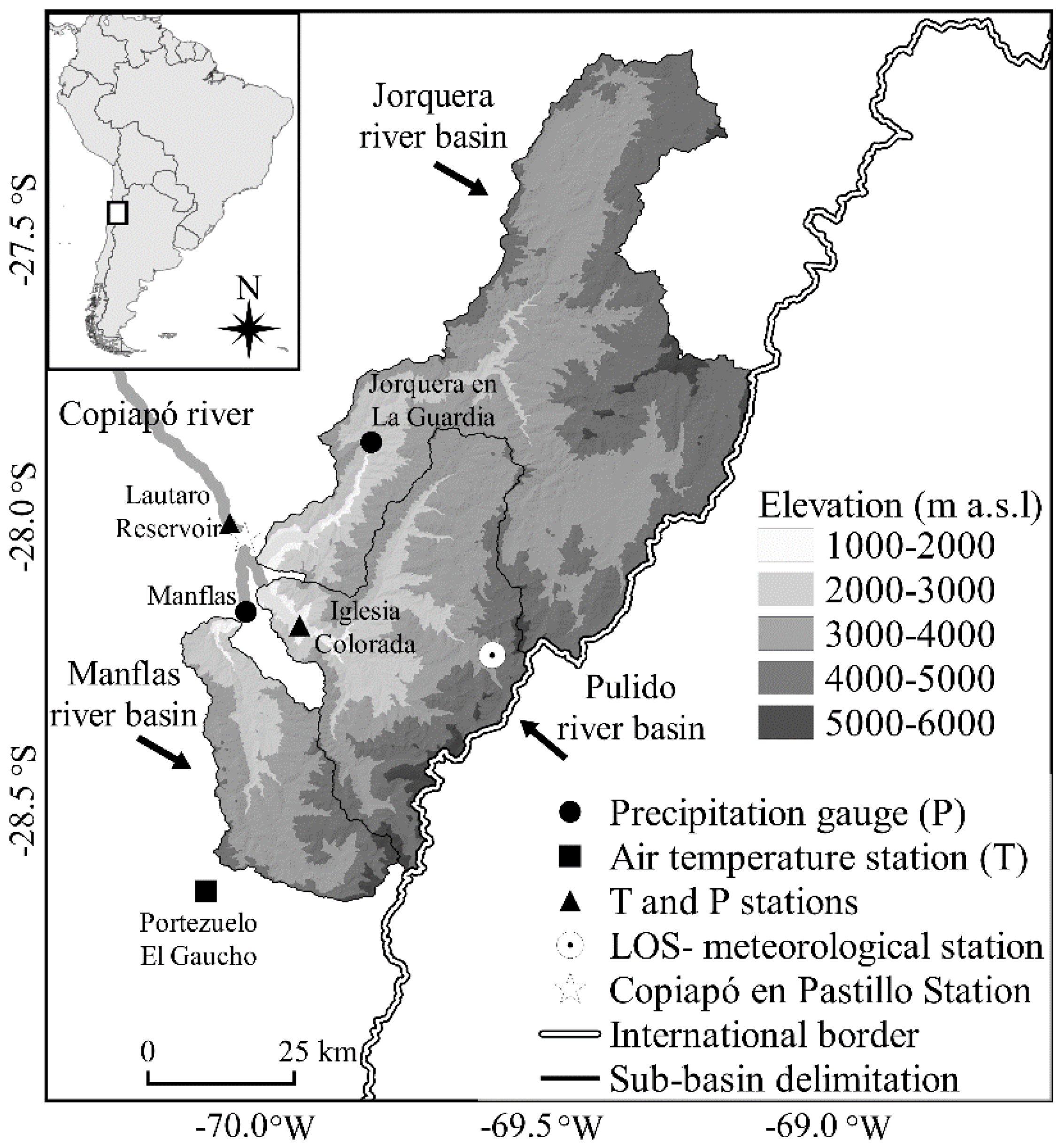
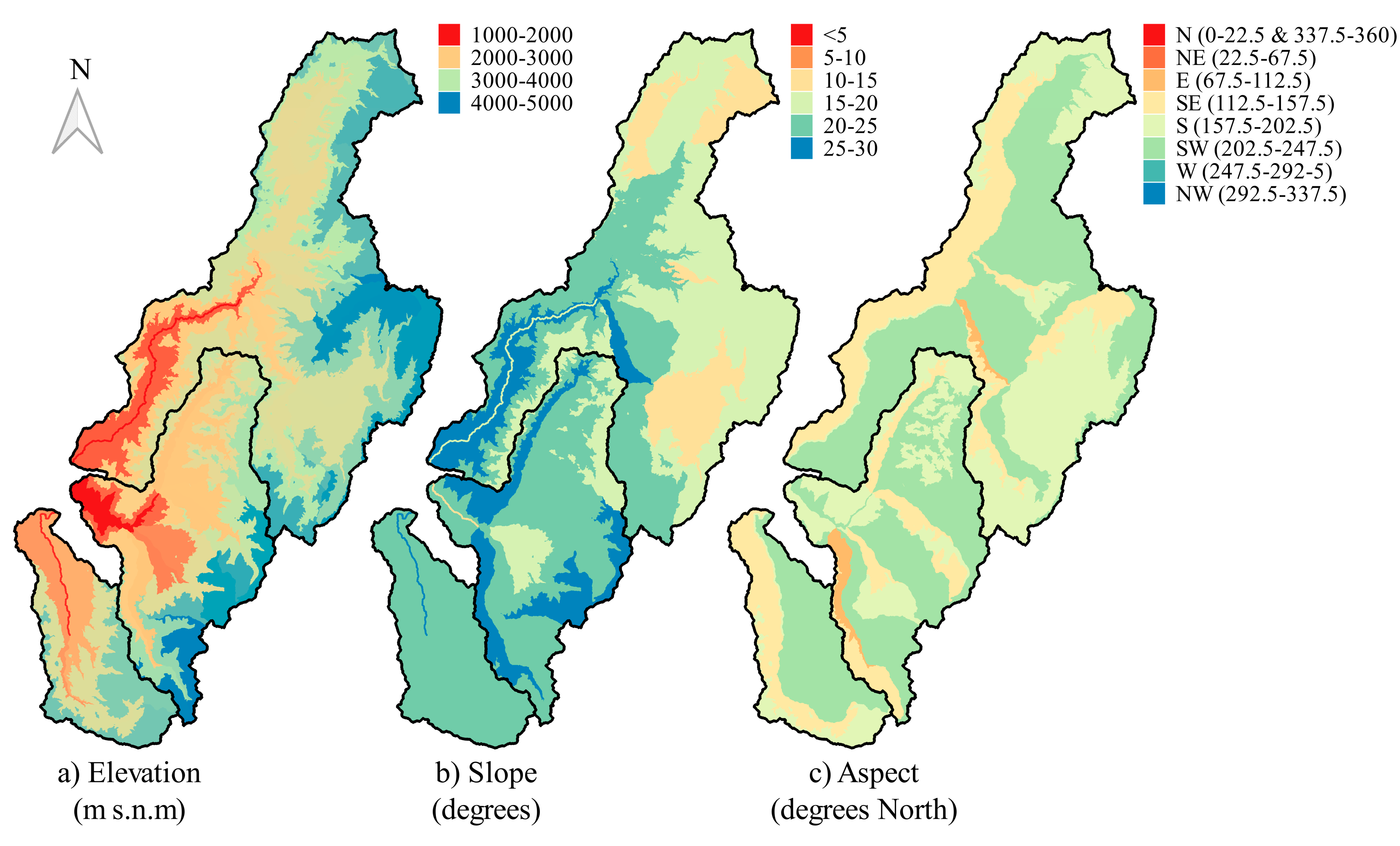
2. Study Area and Available Data

The study site is an extensive arid mountain region in the Atacama Desert, characterized not only by low annual precipitation, but by an excessive water demand from the agriculture and mining industries [11,12]. For that reason, the users of the river are interested to quantify the seasonal snowpack losses coming from sublimation and melting in order to improve the water management. It is likely that the water scarcity in the Copiapó region will be more drastic under climate change conditions, with temperature projections up to +6 °C by the end of the 21st century [13,14,15].

The Upper Copiapó River Basin (UCRB, 70.2°–69.1° W, 27.1°–28.7° S) is a 7194 km² watershed with elevations ranging from 1230 to 6000 m a.s.l. It is formed by the confluence of three rivers: Jorquera, Pulido and Manflas (Figure 1). The climatology of the region is characterized by a short, wet season with an average annual precipitation of 38.8 mm y⁻¹ and a mean annual temperature of 19.9 °C at Iglesia Colorada station (1550 m a.s.l). Rainfall events are highly variable in duration, occurrence, and magnitude year to year [16]. Above 3000 m a.s.l., snow is the dominant form of precipitation. Snow falls as early as April, then snowmelt and runoff occur generally from October to March. The average annual streamflow of Jorquera, Manflas, and Pulido (Figure 1) is 0.2, 0.4 and 0.5 m³/s, respectively. The watershed land cover is mainly barren, although there is some sparse low vegetation, mostly concentrated in gullies and wetlands.

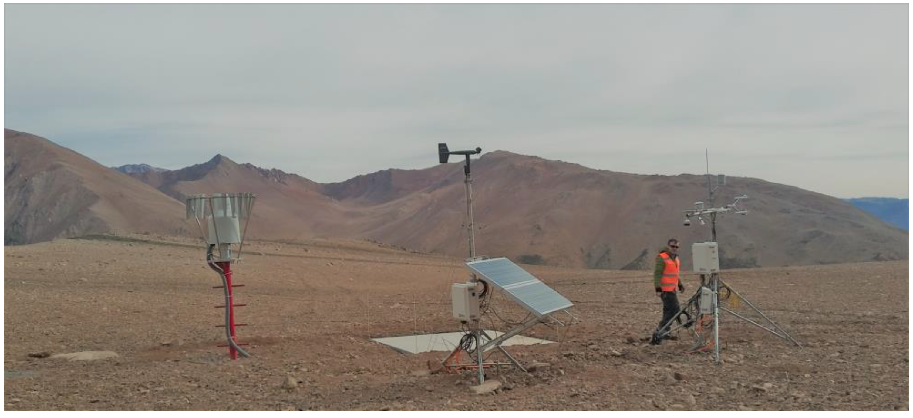
2.1. La Ollita Snow and Meteorological Station (LOS)

A fully instrumented AWS was installed on 15 December 2015 at La Ollita (LOS) site (Figure 2), located at 4320 m a.s.l. (28.21° S, 69.5° W). The station had three major components: energy supply, meteorological station (rainfall gauge, snow pillow) and micrometeorological instrumentation. The energy supply was delivered by two 90 W solar panels placed at 0.7 m above surface level. In addition, a deep cycle battery (80 Ah, 14V) and controller charger provided energy for up to 5 days without recharge. We installed an OTT Pluvio 2 gauge to record the cumulative and differential precipitation over a 2 m mast, including an Alter type wind protection shield. We incorporated antifreeze liquid to avoid accumulated ice inside the rain gauge. In terms of snow measurement, these instruments were complemented by a 3 × 3 m snow-scale sensor, located at the ground level. The meteorological instrumentation included air temperature and relative humidity sensors (Rotronic HC2S3, Campbell Scientific, Logan, UT, USA), a surface radiometric temperature sensor (SI-411, Apogee Instruments, Logan, UT, USA), and a wind speed and direction gauge (05608C, R. M. Young, Traverse City, MI, USA). Finally, the components of the radiative balance were measured by a four-way Net Radiometer (CNR-4 K&Z, Kipp & Zonen B.V., Delft, Netherlands). The measurements were recorded every 30 min in a CR3000 data logger. The eddy covariance sensor (Irgason, Campbell Scientific, Logan, UT, USA) was set up on the same date, however, around two months later, the mast fell unexpectedly before any precipitation event had taken place.

2.2. Hydrometeorological Network

The AWS network from the Chilean national water bureau (Dirección General de Aguas) provided the meteorological forcing for the distributed hydrological model (

Table 1. Automatic weather station (AWS) network used in this study. P: Precipitation, T: Temperature, RH: Relative humidity, ISR: Incident shortwave radiation, U: Wind speed.

Station	Latitude	Longitude	Elevation	Start–End	Measured
Name	(°)	(°)	(m a.s.l.)	date	variable
Iglesia Colorada	−28.1572	−69.8808	1550	1988–2016	P and T
Jorquera en La Guardia	−27.8364	−69.7550	2000	1966–2016	P
Lautaro Embalse	−27.9783	−70.0033	1110	1930–2016	P and T
Manflas	−28.1336	−69.9750	1410	1966–2016	P
Portezuelo El Gaucho	−28.6231	−70.0450	4000	2003–2016	T
Río Copiapó en Pastillo	−28.0003	−69.9747	1300	2013–2016	P
La Ollita	−28.2095	−69.5425	4320	December/15-July/16	P, T, RH, ISR, U

) [17], with a total of seven operational meteorological stations. According to satellite imagery from MOD10A and MYD10A [18] for the period 2001–2015, the mean elevation of the snow line was above 3000 m a.s.l. Notably, all the precipitation gauges were located below 2000 m a.s.l., and therefore there existed considerable uncertainty in the amount and distribution of the precipitation in higher elevations. The synoptic characteristics in the region are favorable to orographic enhancement [19], but also cut-off low pressure systems which produce negative orographic gradients in similar latitudes [20,21].

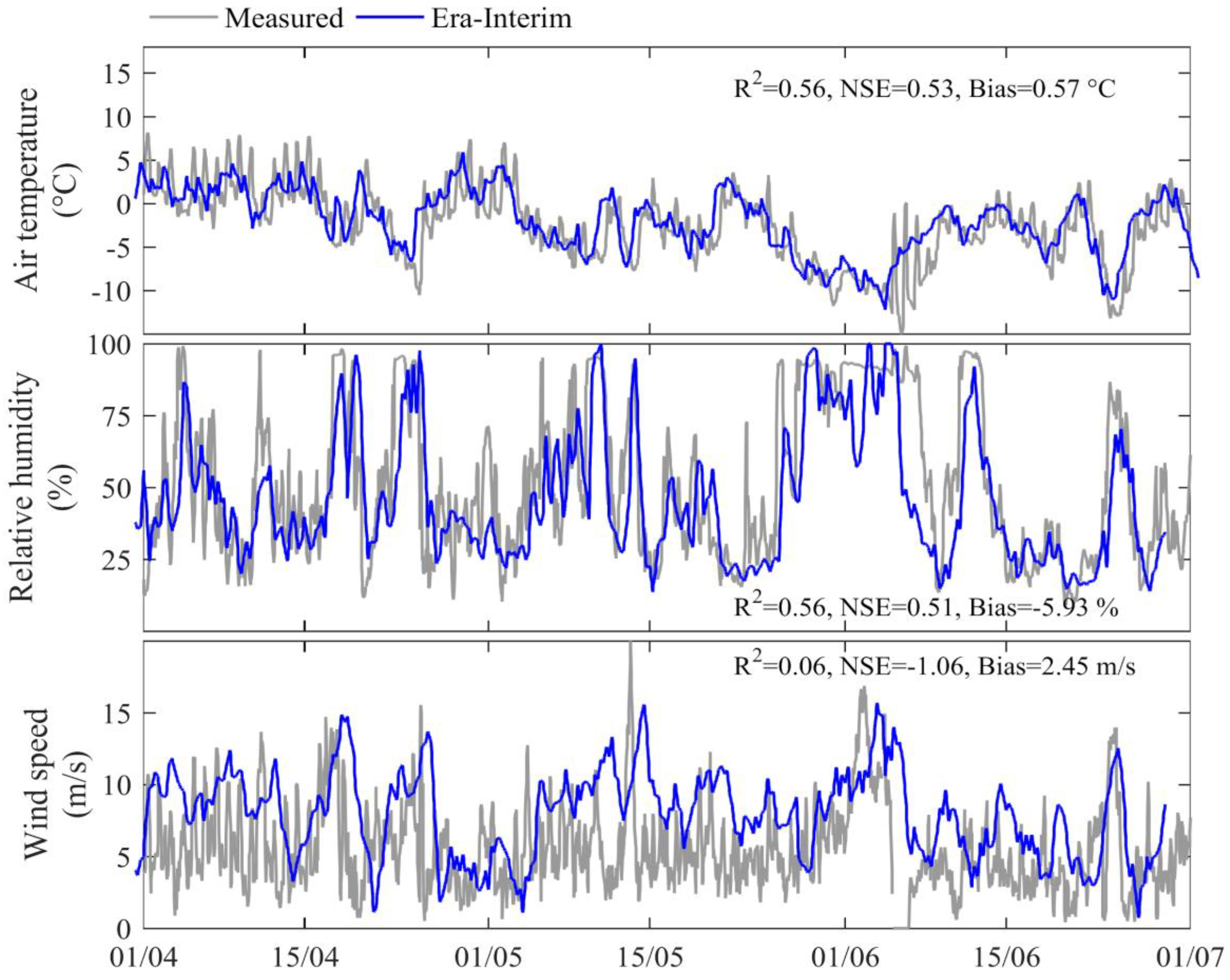
2.3. Reanalysis Data

The AWS’s inconsistent spatial distribution motivated the use of ERA-Interim reanalysis [22] to generate the meteorological forcing for the distributed hydrological model. ERA-Interim is a global atmospheric reanalysis produced by the European Centre for Medium-Range Weather Forecasts [23]. Gridded data products included a large variety of 3-hourly surface parameters and 6-hourly upper-air parameters covering the troposphere and stratosphere [24]. The ERA-Interim configuration has a spectral T255 horizontal resolution of 0.7° uniform grid (approximately 79 km) and 60 levels in the vertical, and the products are interpolated to resample the original grid using bilinear methods [22].

3. Methodology

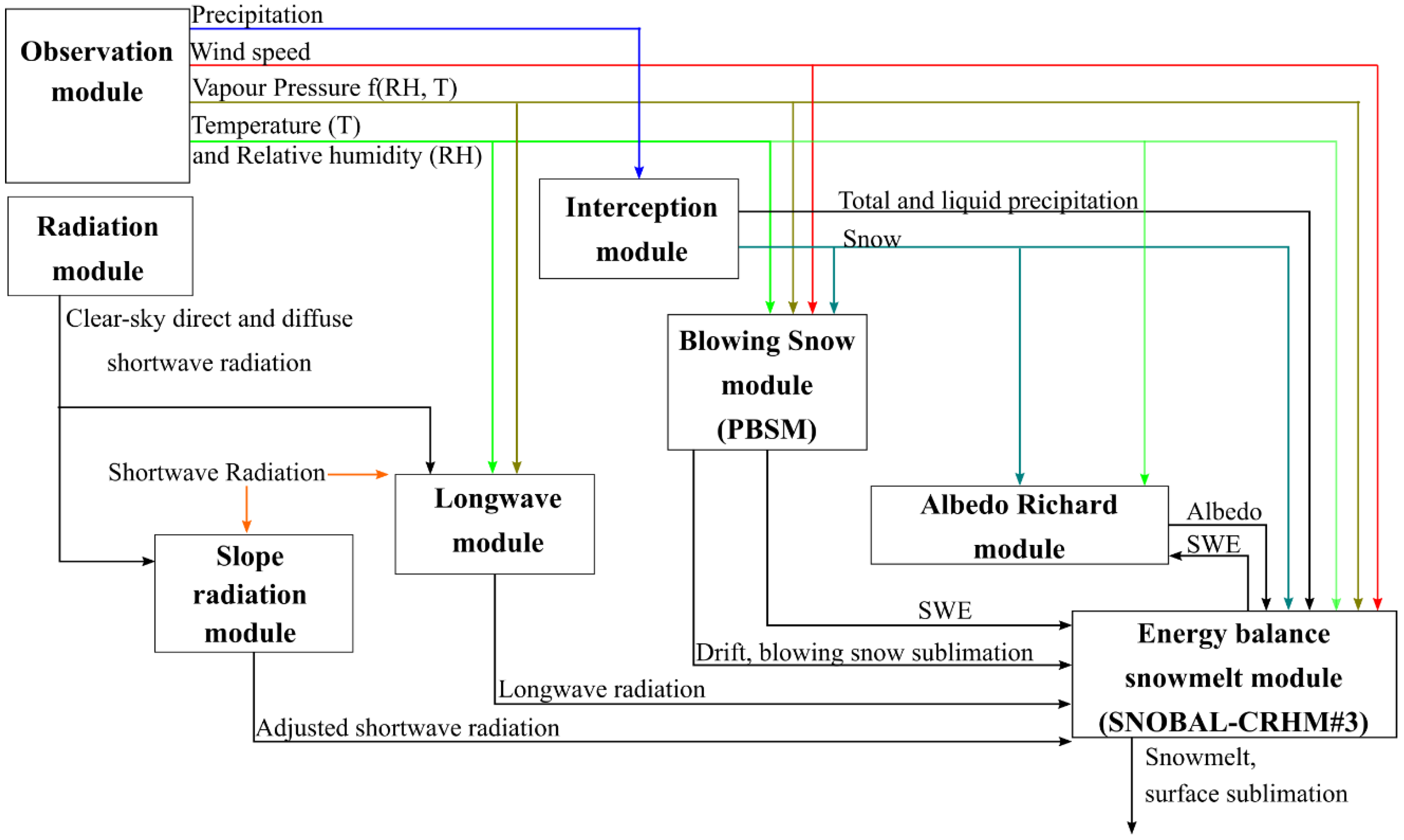
3.1. Snow Mass Balance Model

Snow processes were computed using the Cold Regions Hydrological Model (CRHM) [10], which employed a modular structure to simulate the sequence of processes of accumulation and ablation of snow. First, we ran a site-scale model at LOS with hourly observed data for the year 2016 including precipitation, air temperature, relative humidity, wind speed and incident shortwave radiation. The model parameters were set according to previous publications (see References in

Table 2. Parameters applied in Cold Regions Hydrological Model (CRHM) for the site-scale model and distributed hydrological model. UCRB: Upper Copiapó River Basin. LOS: La Ollita station.

Parameter	Description	Value	Units	Reference	Module
${\alpha }_{max}$	Maximum Albedo for fresh snow	0.85	-	[26]	Albedo
${\alpha }_{min}$	Minimum Albedo for aged snow	0.5	-	[27]
$\tau$	Albedo decay for cold snow	$1.2\times {10}^6$	s	[26]
$s_{min}$	Minimum snowfall amount required to refresh the albedo to ${\alpha }_{max}$	1	mm	Calibrated
$F$	Fetch length	LOS: 650 m UCRB: 1500 m	m	Calibrated	PBSM
${\rho }_{snow}$	Snow density of falling snow	100	kg m−3	[28]	SNOBAL
$max\_H_2{O}_{vol}$	Max liquid water content as volume ratio	0.01	-
$max\_z_{s0}$	Maximum active layer thickness	0.1	m
$z_0$	Roughness length	0.001	m

), but others such as the minimum snowfall to refresh the albedo and the fetch length were calibrated. We applied the Nash–Sutcliffe coefficient (NSE) [25] as a metric to calibrate the in-situ Snow Water Equivalent (SWE). The precipitation phase in CRHM was determined using a mixed-phase approach based on air temperature, considering a linear transition zone between 0 and 2°C. If the temperature was below this range, the precipitation was considered snowfall, and above 2 °C was considered rainfall.

Arranged within CRHM is the Prairie Blowing Snow Model (PBSM) [4] which simulates snow drift and blowing snow sublimation. Owing to the barren land cover of the region, the only relevant parameters for the PBSM were the fetch length and the distribution factor for snow transport. For the site-scale model, fetch length was determined using the dominant wind direction and field observations at the site, leading to a fetch value equal to 650 m, comparable in order of magnitude to small catchments [29]. Due to the topographical setting of the site (no obstacles on the predominant windward direction and low slopes leeward), it was simulated as an outgoing drift source. Snow albedo was parameterized with an exponential decay curve during the melt period [27]. DeBeer and Pomeroy [26] proposed arbitrarily an albedo decay equal to $\tau ={10}^6$ s, whereas Essery and Etchevers [27] calibrated $\tau$ for various cold regions of the world ranging between $7.2\cdot {10}^5$ and $1.8\cdot {10}^6$ s. We used $\tau =1.2\cdot {10}^6$ s which was close in magnitude to [26] and in the upper range of [27]. The maximum albedo for fresh snow was set at 0.85 and the minimum snow albedo to 0.5, following [27]. The value of $s_{min}$, the minimum snowfall amount required to refresh the albedo, was adapted to 1 mm to achieve a realistic albedo given the low precipitation climatology in the region. With higher $s_{min}$, similar to other studies (e.g., [27,28,29,30]), the albedo was not responsive to new storms. This parameter was above the reported precision of OTT Pluvio2 pluviometer [31].

Additionally, the SNOBAL parameters were defined as the defaults suggested by Marks et al. [28,32]. The maximum active layer thickness was first set to 0.25 m by [28] but afterward [32] found that setting it to 0.1 m improved the simulation of turbulent fluxes. The roughness length (z₀) was set to $1\cdot {10}^{-3}$ m, which was a realistic value for snow surfaces, following [33] and [34]. According to the simplified scheme proposed by Paeschke [35], we estimated that with an average grain size of about 3 cm the roughness length was $4\cdot {10}^{-3}$ m. The lack of vertical profiles of wind speed and air temperature prevented the calculation of surface instability, stress velocity, and therefore roughness.

The different modules in CRHM are linked to each other, first processing the meteorological forcing and then transferring the results to the following module (Figure 3). This sequence was applied for the UCRB distributed model and the site-scale model for LOS.

3.2. Distributed Hydrological Model

We built a spatially distributed snow model in CRHM for the UCRB in order to evaluate the importance of energy and mass fluxes at the catchment scale. CRHM was run for the period 1 April 2001 to 31 March 2016 at an hourly time step. For the analysis, the UCRB was divided into catchments: Jorquera, Pulido and Manflas (Figure 1). Each subcatchment was then discretized into hydrological response units (HRU), employing the physiographic characteristics expected to play a significant role in snow accumulation and ablation such as elevation, slope, and aspect (Figure 4), derived from the SRTM digital elevation model with 1 arc-second resolution. The HRU delineation was based on the following criteria: (i) division of the sub-basins, (ii) equal elevation bands for each sub-basin delimited in the previous step, (iii) division by sides of river and the aspect and (iv) a riverbed buffer of 200 m at the end of the river. The UCRB basin split into 81 HRU: 43 in Jorquera, 31 in Pulido and 7 in Manflas. For each HRU, the meteorological forcing and hydrological parameters were spatially homogeneous and therefore, the same hydrological processes were dominant.

Based on satellite imagery [36] and the land use of the basin, we set barren cover to each HRU above 3500 m a.s.l., where there were not significant boulder fields. For that reason, the only relevant parameters for the PBSM model were fetch length and the distribution factor for snow transport. A constant fetch length of 1500 m was adopted for each HRU in the UCRB, mainly due to the lack of wind direction measurements in the study period; however, we discuss possible consequences of this decision in the Section 5.2. A uniform distribution factor was assumed for the HRUs above 3500 m a.s.l., meaning those HRU may have received or delivered transported snow. Below this elevation, the drifted snow was deposited.

The ERA-Interim 6-hourly (06, 12, 18 and 24 UTC) air temperature and relative humidity was obtained for each HRU, based on the interpolated grid of 0.125° × 0.125°, considering pressure levels 600, 650, 700, 800, 850, 900 and 925 hPa from April 2001 to July 2016. An elevation correction for air temperature was implemented using the Lapse Rate methodology [37]. In this approach the ERA-Interim air temperature at a certain geographical elevation is defined through Equation (1):

$$T_{ERA-Interim}=T_{pressure-level}+\Gamma \cdot \Delta z$$

(1)

where $\Delta z=z_{DEM}-{\varphi }_{pressure-level}/g$ in meters, $z_{DEM}$ is the elevation of 1 arc-sec SRTM digital elevation model $\left(m\right)$, ${\varphi }_{pressure-level}$ is the average geopotential height of the pressure level (${\mathrm{m}}^2{\mathrm{s}}^{-2}$), $g$ is the acceleration of gravity ($9.81 \mathrm{m}{\mathrm{s}}^{-2}$). $T_{pressure-level} \left(°\mathrm{C}\right)$ was defined as the closest pressure level temperature respect to the DEM elevation, that is when $\Delta z$ is minimum. The lapse rate $\Gamma$ was calculated as the difference between the highest (600 hPa) and the lowest (925 hPa) level pressure air temperature. Then, we applied the nearest neighbor downscaling for each HRU centroid. Similarly, the relative humidity was determined using the closest pressure level respect to the DEM elevation with the nearest neighbor downscaling to each HRU centroid.

We generated an a-priori distribution of incoming solar radiation ($I{S}_w$) from the DEM using GRASS-GIS software, which considered the effect of the latitude, aspect, and slope. The solar radiation of each HRU ($I{S}_{w-@URH}$) was normalized by LOS’s nearest pixel ($I{S}_{w-@LOS}$). Finally, the incident shortwave radiation was calculated as the ERA-Interim time series radiation at LOS ($I{S}_{w-ERA@LOS}$) weighted by the normalized radiation ($I{S}_{w-ERA@LOS}\cdot I{S}_{w-@URH}/I{S}_{w-@LOS}$).

Wind speed was estimated based on the 10-m U and V wind components of the ERA-Interim 3-hourly data, downscaled to the centroid of each HRU through a nearest neighbor algorithm. Hourly data for air temperature, relative humidity, wind speed and shortwave radiation were calculated as the linear interpolation of the 6-hourly or 3-hourly data. Precipitation data were estimated using a reference station from each subbasin: Jorquera (Jorquera en La Guardia station), Pulido (Iglesia Colorada station) and Manflas (Manflas station). Observed daily precipitation data were extrapolated to the entire catchment using orographic weighting factors determined from the national annual precipitation official isolines, issued by the Chilean water authority [38]. This precipitation distribution is commonly used in local studies with sparsely gauged basins in the Chilean Andes, providing adequate basin-scale estimates which match observed water budgets (e.g., [39]). Hourly data were obtained based on the hourly statistics from 57 storms at the Río Copiapó en Pastillo station. Due to the proximity of the reference stations, it was assumed that the same relationship holds between storm length and precipitation amounts; thus, from daily precipitation values at the reference stations, both storm length and hourly precipitation were derived.

To validate the distributed snow model, we compared modeled fSCA and MODIS snow cover products. The simulated fSCA was reconstructed using SWE, each HRU was flagged as snow covered when the simulated SWE was greater than 1 mm, similar to [8]. This rather crude approach allows us to estimate catchment-scale fSCA as the area-weighted average of HRU fractional snow cover. We compared this catchment-scale value with the daily MODIS fSCA at 500 × 500 m resolution, obtained as a combination of MYD10A and MOD10A products [18].

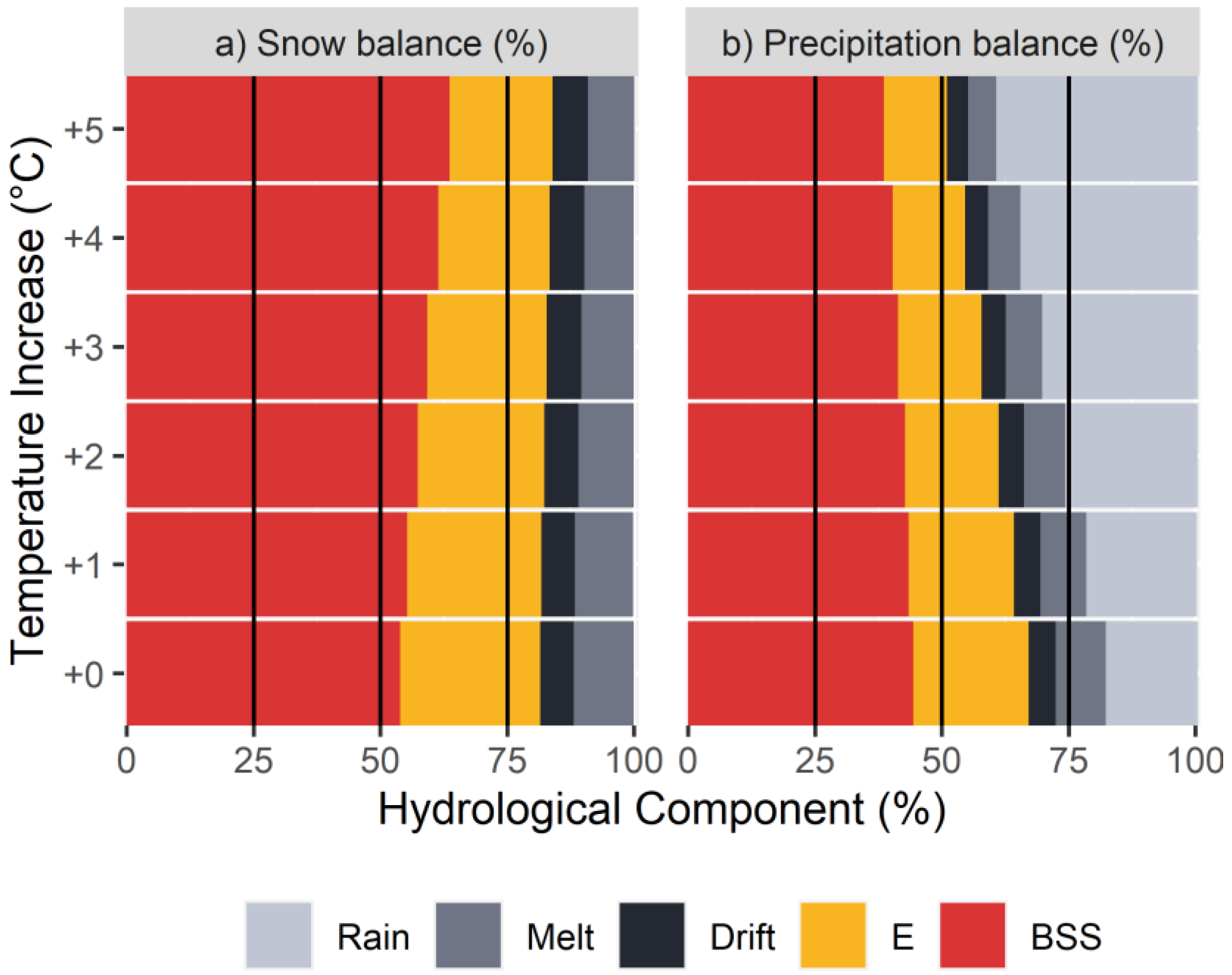
3.3. Climate Sensitivity Analysis

Most of the RCP8.5 climate projections for the north of Chile had forecasted incremental trends in temperature, ranging from 0 to +5 °C at the end of the 21st century in the Copiapó region [15]. We performed a sensitivity analysis of the snow ablation components (blowing snow sublimation, surface sublimation, melt and snow drift) by perturbing air temperature in the climatological period 2001–2016.

4. Results

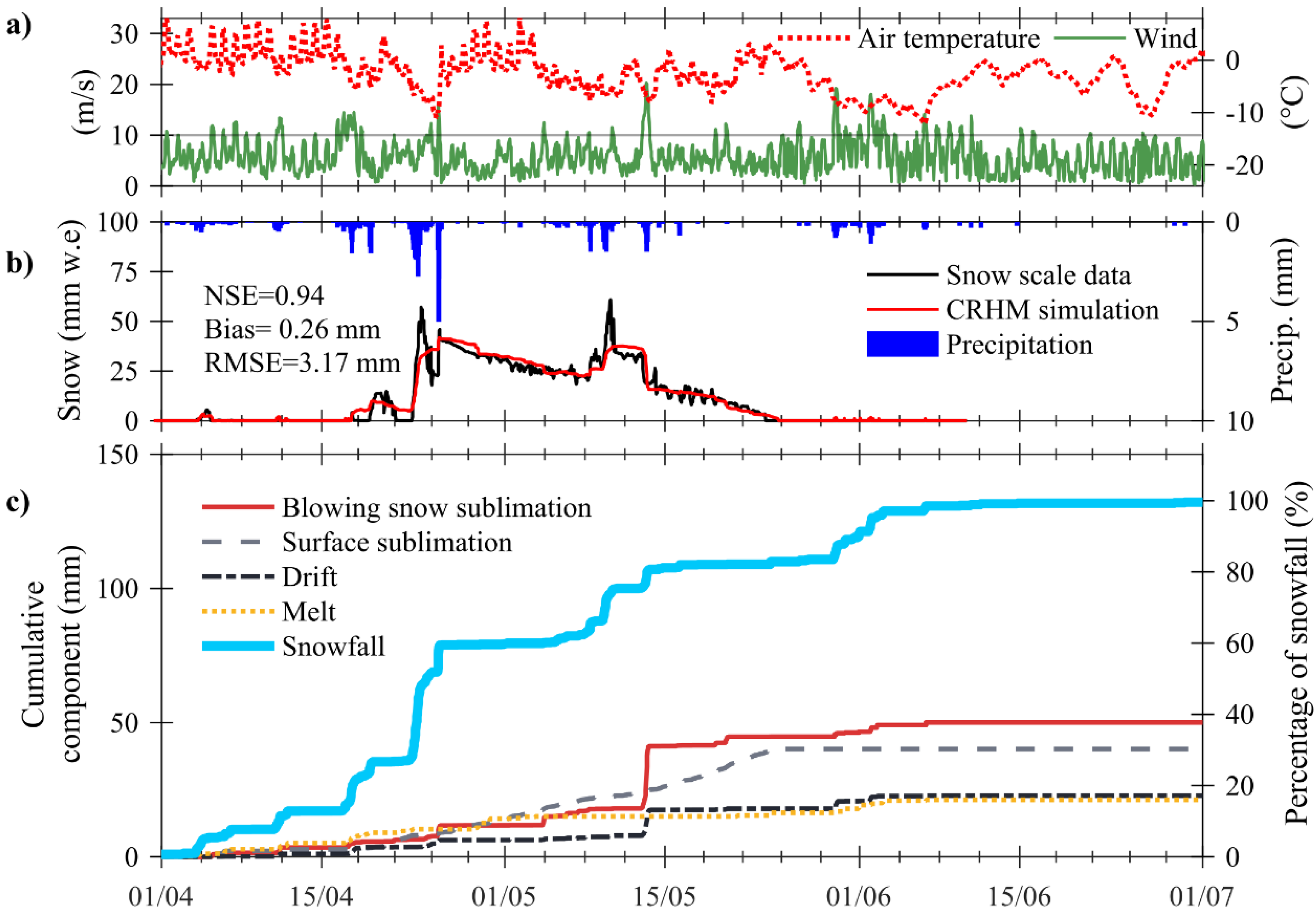
4.1. Simulations at LOS

We simulated the snow processes by employing LOS’s in-situ measurements between April and July 2016 (Figure 5). The snowpack (SWE) was calibrated using the snow scale measurement (Figure 5b). The model reproduced the snowpack dynamics during this period with a Nash–Sutcliffe efficiency of 0.94 and an RMSE of 3.17 mm, showing a bias of 0.26 mm. Even though the highest peak in snow accumulation of 57 mm was missed by the model, the difference between the observed and simulated SWE was not larger than 5 mm in the following days. Importantly, the simulated SWE decay slope matched to the observed data, especially after snowfalls.

At the station, the observed accumulated precipitation was nearly 132 mm (Figure 5c), distributed along the season in minor events. Two major storms accounted for most of the snowpack in the season: 24 April 2016 and 13–15 May 2016. In the first major snowfall, the snowpack melted rapidly, as air temperature was near 0 °C and wind speed lower than 10 m s^-1. It accounted for 40 mm in SWE with a similar share of losses between the ablation snow components. Between 13 and 15 May 2016, the snowfall added roughly 25 mm of SWE (Figure 5b), completing around 45 mm in the snowpack. However, on this occasion, as wind speed was greater than 20 m s⁻¹, nearly 10 mm drifted off the site and blowing snow sublimation was up to 25 mm. After 15 May, the snowpack continued to disappear at an almost constant rate of surface sublimation, finishing the snow cover on the 23 May. Finally, a storm of almost 20 mm on 29 May 2016 did not accumulate significant SWE, due to a combination of wind speed over 15 m s⁻¹ and temperatures below −5 °C, leading to the erosion of the snowpack by blowing snow sublimation and transport.

CRHM results at LOS suggested that blowing snow sublimation was the most significant component of the mass partition in the 2016 season and it accounted for almost 36% of the snowfall losses between April and July. Nearly half of this amount can be attributed to the 13–15 May event with strong wind speed and low temperature. Equally, surface sublimation losses were 30% of the snowfall, while drift and melt each represented approximately 17% of the ablation during the season.

As a way to assess the distributed meteorological forcing from ERA-Interim, we compared the measurements at LOS with the 0.7° pixel in ERA-Interim, including air temperature, wind speed and relative humidity (Figure 6). In general, ERA-Interim represented the average meteorological conditions at LOS of temperature and relative humidity, but not the intraday variability. The temperature, precipitation and wind speed biases were 0.57 °C, −5.93% and 2.45 m s⁻¹, respectively, and the determination coefficient was 0.56 for both air temperature and relative humidity. However, the modeled wind speed’s R² was 0.06, poorly representing the intraday cycles and biased positively.

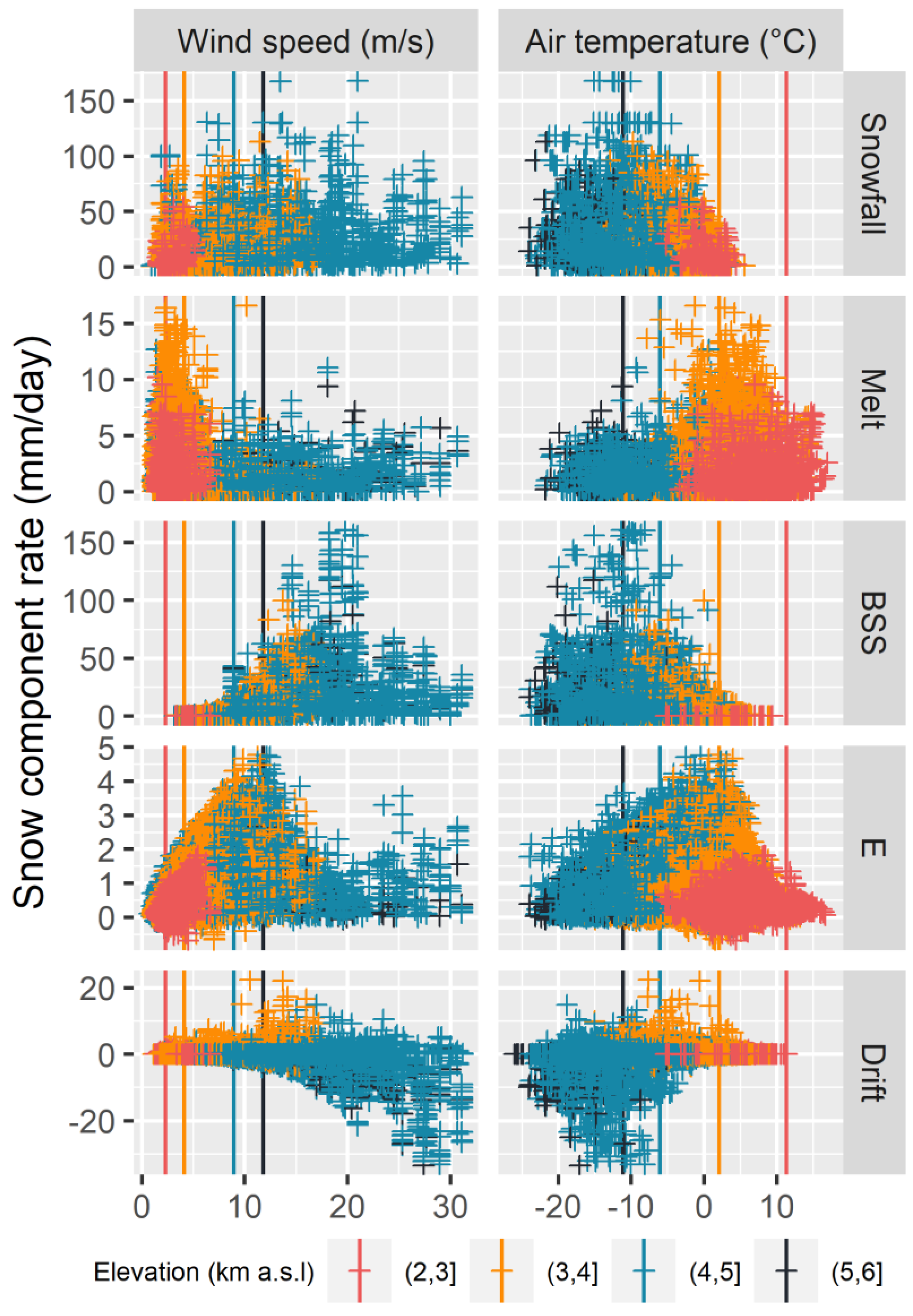
4.2. Simulations at Catchment-Scale

The fractional snow cover area was compared in order to verify the snow distribution along the basin and seasonal duration coherence. Contrasting MODIS imagery and simulated snow cover revealed a moderate correlation with coefficients of determination of 0.58, 0.50, 0.61 at Jorquera, Pulido and Manflas basins, respectively, (See Figure S1 for time series). Because of the difference in spatial resolution in these two approaches (kilometric HRU vs. 500 m pixels), this exercise was considered as a rough assessment of the snowpack extension and duration at the catchment level.

Simulations of the average monthly snow balance indicate that in Jorquera and Pulido blowing snow sublimation represented half of the wintertime ablation for the period 2001–2016, while in fall and spring (March to April and September to November) the melted snow signified up to 40% of the ablation (Figure 7). In Manflas, however, the melted snow reached up to 75% of snow ablation in the driest months of the year (October to February) and blowing snow sublimation was lower compared to the other basins, which is attributed to the relatively higher temperatures of the basin and lower wind speeds (lowest-elevation basin). On the other hand, surface sublimation remained in the range 5 to 7.5 mm/month across the three basins, declining in spring and summer given the retreat of the snow cover, where melting began to dominate the snow mass balance as the radiation was higher.

The elevation influenced the snow dynamics due to the spatial variability of the meteorological forcing (Figure 8). At the lowest band (2000–3000 m a.s.l.), wind speed never reached 10 m s⁻¹ and air temperature was generally greater than 0°C in 2001–2016, which provided conditions for higher daily rates of melt and surface sublimation. Generally, melting rates were lower than 15 mm/day and 3.5 mm/day of surface sublimation below 4000 m. Even though this range of elevation concentrated the least volume of snow (Figure 9), following the orographic effect implemented in the precipitation distribution scheme. The blowing snow mechanisms increased in rates and volume with the elevation, influenced by the higher wind speeds and lower temperatures, whereas snow melting and surface sublimation tended to decrease in rates and volume above 4000 m (Figure 8). Blowing snow sublimation represented 73% of the snow volume between 4000 and 6000 m (Figure 9c). The transported snow rates increased in a cumulative normal distribution above 5 m s⁻¹ wind speed, as a direct consequence of the probability of blowing snow and a higher boundary layer in PBSM [5]. The simulated rates of drifted snow in high elevations (4000–6000 m) went up to 28 mm/day and accounted for around 10% of the snowfall’s volume. As implemented in the model, the snow in high elevations was redistributed to the surroundings or to lower elevations, which produced a reception of transported snow up to 20 mm/day in the 3000–4000 m level.

The sensitivity analysis of the temperature indicated a general decrease in the availability of snow due to a rise (reduction) of liquid (solid) precipitation by 4% °C⁻¹ (Figure 10b). Previously, other studies have noticed a projected reduction in the snowpack per degree increase of 10% °C⁻¹ in Svalbard [40] and 15% °C⁻¹ decline in the Swiss Alps [41]. [42] conducted a statistical sensitivity analysis for 44 mountain regions in the world under warmer conditions, which suggested that places with cold winters (mean lower temperatures than −8 °C) did not respond significantly to changes in rainfall ratio (~ +5% per C°) and presented insensitive snowpack peaks and snow duration.

In the snow balance, the least affected components under warming conditions will be transported and melted snow (Figure 10a). Surface sublimation, however, will be reduced by 1.5% per degree increase, as this component is dependent on the duration of the snowpack. Blowing snow sublimation will increase in a warmer climate as a percentage of the snowpack (+2% per degree increase), but as the rainfall ratio will be more significant in terms of the precipitation, less blowing snow will be available to sublimate.

The monthly UCRB’s average snow cover area between 2001 and 2016 (SCA, Figure 11a) revealed an expected seasonal snow between April and September, that peaked in July where 25% of the basin was covered by snow. In warmer conditions, the fraction of SCA will decline by 2% per degree increase during winter (Figure 11a), which represents nearly 145 km² °C⁻¹ of less snow at UCRB.

The seasonal snowpack duration widely fluctuated year to year (Figure 11b). Between 2001 and 2015, the driest year offered only 36 days of snow, whereas the wettest year reached up to 225 days. The average duration of the snowpack declined steadily under warmer climate, almost 6 days or −5% °C⁻¹. The wettest years were more susceptible to reductions, whereas in the driest years the seasonal duration will remain approximately constant. Other regional studies, such as [42], projected a reduction in snow duration in 44 basins of between 2 and 27% per degree increase, and remarkably, a similar location in the semi-arid Andes of Chile anticipated −5.5 days °C⁻¹ [43], while other locations in the same study expected at least 25 days °C⁻¹ less.

The annual peak SWEs at UCRB ranged from 4.7 to 140.0 mm in the simulation period, with a median of 26 mm and an average of 43 mm (Figure 11c). Under a warmer climate, the 75th percentile exhibited a sharp reduction of −5.3 mm °C⁻¹, whilst the declination of the mean was roughly -3.4 mm °C⁻¹; or 7.9%°C⁻¹. The maximum SWE in the driest years remained almost constant with temperature increment (−0.5 mm °C⁻¹). [42] observed a large variability in the response of the peak SWE to warmer climates in different basins, with a decrease between 0.3 and 45% per °C.

5. Discussion

5.1. Meteorological Uncertainties

Due to the scarce coverage of instrumentation in the north of Chile, one of the prevailing sources of uncertainty is the spatial distribution of meteorological variables. This condition limits the reliability of snow mass and energy simulations in the Dry Andes. In this study, the precipitation parametrization based on AWSs and the orographic enhancement affected the simulated snow in magnitude and distribution. In Copiapó, frequent winter cold fronts are expected from the Pacific [44], characterized by westerly and southerly flows which lead to a prominent positive latitudinal height gradient in the Andes [19,45,46]. This precipitation distribution is due to the South East Pacific Anticyclone [47,48] that normally prevents convective precipitation due to subsidence [21]. Low frequency events were neglected in this study, such as cutoff lows [20], which feed anomalous events of convective precipitation in austral summer and temporarily reverse the precipitation gradient (e.g., [21]). Furthermore, global reanalyses used to compensate the lack of stations in remote regions still present large bias in precipitation in the Dry Andes and moderate correlation with annual observations [49,50], which brings substantial uncertainty in high-elevation snow simulations [8,9]. Additionally, the precipitation gauge measurements in the AWSs network could be underestimated, owing to the physical constraints of the instruments in capturing precipitation in the surrounding area, especially during snowfall and windy storms [51,52]. More studies exploring gridded modeled precipitation in the area, such as Weather Research and Forecast model (WRF) and under catch corrections, are required to study the precipitation distribution effect.

Snow processes are highly sensitive to wind as turbulent energy fluxes and blowing snow directly depend on the magnitude of wind speed [4,32]. Wind fields are, however, one of the hardest variables to be estimated, given the complexity of air motion in mountain regions and the unavailability of long-term records to assimilate global reanalyses [53]. Micrometeorological models can be applied to simulate synoptic wind, but they tend to be more unreliable in local wind fields such as katabatic and anabatic winds [8]. We acknowledge a possible positive bias in wind speed derived from the ERA-Interim product, and therefore in the blowing snow processes, as the comparison with the local station LOS presented a bias of around 2.5m s⁻¹ for the season 2016. This is a similar to the error expected in the WRF model for wind energy applications in Chile [54].

Air temperature is one of the main driving forces in the snow ablation process, and is partly responsible for the changes in sensible energy flux, air density, relative humidity, vapor pressure deficit and therefore, directly related to the sublimation and snow melt [4,32]. The temperature from the ERA-Interim reanalysis generally presents an agreement with the local station in magnitude and variability in high Andes areas [49] and for the current applications in macroscale, the parametrization of the temperature provides reliable magnitude and temporality.

5.2. Model Limitations

The PBSM model was originally designed for the Canadian Prairies, which are characterized by relatively flat terrain and homogenous vegetation [4]. The model equations are resultant from field observations, idealization of snow particles in the air and thermodynamic equilibrium [4,5,55]. One of PBSM’s highlighted assumptions is the development of the snow processes within a stable boundary layer (comprised by a saltation and suspension layer) in the wind predominant direction [5]. The suspension boundary layer is highly sensitive to fetch after a threshold of wind speed (greater than 8 m s⁻¹, Pomeroy, 1988). The PBSM equations are integrated along the fetch and boundary layer, an increase in each of them translates in more blowing snow to sublimate.

In this study, the LOS is located in an exposed and relatively flat area that allows wind to flow for at least 500 m without obstacles. However, the topography of the catchment is complex and diverse, and for that reason we applied a uniform fetch length in each HRU to compensate for the topography effect of the mountains and the lack of wind directions across the large scale of the basin. As we are interested in the macroscale system, the current model is sufficient to estimate the ablation components in the areal average of each HRU, as the SCA of the basin showed a reasonable coherence with satellite imagery. The implications in the snow model are that a longer fetch will increase the blowing snow sublimation, and the inverse is also valid. Fetch length in exposed areas generally range from 300 to 3000 m in other basins [56,57]. Several PBSM-SNOBAL-CRHM models have been successfully applied in mountainous conditions, such as subarctic mountains [29], the Canadian Rocky Mountains [58], Yukon river in Canada [59], Patagonia [60] and in particular, applied for sensitivity analysis in various mountain regions around the world [42,43].

5.3. Potential Impact of Warmer Conditions

Air temperature is highly embedded within PBSM and SNOBAL in non-linear functions, where the blowing snow sublimation rate is modeled as a snow spherical particle that gains or losses mass from solid to water vapor at a rate of $dm/dt=f\left(T\right).$ This rate is integrated along the fetch and the boundary layer, which are independent of air temperature. Additionally, the perturbation of air temperature alters some snow properties, such as longwave radiation, energy fluxes (especially sensible heat and melting rates) and the rainfall ratio. In this study, relative humidity remained unchanged, supported by the low relative humidity change projected by 1% K⁻¹ [61] and allowed water vapor pressure to vary in a coherent way with temperature changes (following [43,59]). Under warmer conditions, a decrease in snowpack was expected, due to an increment in latent heat of fusion, which in CRHM was modeled as more precipitation falling into the liquid–solid transition phase between 0 and 2°C, or higher. The remarkable result is that phase change is the most sensitive process in the mass balance compared to ablation components. The different snowpack sensitivity analyses showed a low response to warmer climates, in terms of the snow duration, snow depth, SCA and slight fluctuations in ablation components. This phenomenon has been observed in other cold regions where the average temperature May–December (November–June for Northern hemisphere) is less than −5 °C [42,43], which was the range of temperatures above 4000 m a.s.l. in this study (Figure 8). Below 4000 m a.s.l., the rainfall ratio is highly susceptible to perturbations in air temperature; thus, it is expected to be the most vulnerable region to climate change.

5.4. Snow Ablation Results in Other Studies

Snowmelt was the smallest fraction of snow mass across the catchment for the period 2001–2015 and the season 2016 at LOS, even though it was highly relevant when wind speed was under 5 m s⁻¹ and air temperature around 0 °C. Those conditions were normally met in areas below 4000 m with rated of melt up to 15 mm/day and where melt represented 25% of snowfall.

Due to the orographic gradient of precipitation, the region above 4000 m received 63% of snowfall volume. At these elevations, the average temperature in the period May–December was below −6 °C and wind speed over 9 m s⁻¹ (Figure 8), which explained the predominant importance of blowing snow sublimation and secondarily, surface sublimation. These large sublimation losses have been reported in other studies in the semi-arid Andes such as [3] with 81% of the ablation in Guanaco Glacier and over 70% in Pascua-Lama [8]. Ref. [9] in La Laguna basin estimated around 80–86% of sublimation when WRF forcings were applied and 42–49% of sublimation with station-based forcing and [43] found an expected 39% of sublimation in Tascadero (31° S). In general, the consensus to explain the high sublimation in the Andes is that storms are restricted to the coldest months, combined with high incoming solar radiation, low relative humidity, and high wind speeds [3,8,43,62,63]. Further studies with long term measurement of the energetic fluxes and blowing snow are required to validate the simulation applied in these rare regions, which might test the simplifications and limited capacities of the current snow models.

6. Conclusions

This work has presented a physically based distributed snow hydrology model for an arid mountain river system, with parameters derived from short-term observed data and forced with a combination of observed and reanalysis meteorological inputs. The ability to use directly observed parameters within the model, with minimum calibration, increased our confidence in the estimations, as we extrapolated model parameters in space and time. In this extreme environment, it was estimated that surface and blowing snow sublimation played a significant role in the water budget, representing more than 70% of the snow balance over the 16-year period between 2001 and 2016.

The sensitivity analysis showed that under warmer conditions, a larger fraction of precipitation may be available in the form of water resources, due to two effects: (1) a larger rain ratio, and (2) a relative insensitivity of the snowpack in high elevations. Potentially, the available rain could infiltrate and become part of the groundwater system, which currently is the most relevant form of water supply in the Copiapó. Future work should aim to unravel the interplay between snowmelt, river flow, and natural groundwater recharge, in order to better understand the possible feedback of climate change effects, which can yield better predictive models for water resource planning.

References

1. Barnett, T.P.; Adam, J.C.; Lettenmaier, D.P. Potential impacts of a warming climate on water availability in snow-dominated regions. Nature 2005, 438, 303. [Google Scholar] [CrossRef]
2. Hoffman, M.J.; Fountain, A.G.; Liston, G.E. Surface energy balance and melt thresholds over 11 years at Taylor Glacier, Antarctica. J. Geophys. Res. Earth Surf. 2008, 113. [Google Scholar] [CrossRef] [Green Version]
3. MacDonell, S.; Kinnard, C.; Mölg, T.; Nicholson, L.; Abermann, J. Meteorological drivers of ablation processes on a cold glacier in the semi-arid Andes of Chile. Cryosphere 2013, 7, 1513. [Google Scholar] [CrossRef] [Green Version]
4. Pomeroy, J.W.; Gray, D.M.; Landine, P.G. The prairie blowing snow model: Characteristics, validation, operation. J. Hydrol. 1993, 144, 165–192. [Google Scholar] [CrossRef]
5. Pomeroy, J.W.; Li, L. Prairie and arctic areal snow cover mass balance using a blowing snow model. J. Geophys. Res. Atmos. 2000, 105, 26619–26634. [Google Scholar] [CrossRef] [Green Version]
6. Reba, M.L.; Pomeroy, J.; Marks, D.; Link, T.E. Estimating surface sublimation losses from snowpacks in a mountain catchment using eddy covariance and turbulent transfer calculations. Hydrol. Processes 2012, 26, 3699–3711. [Google Scholar] [CrossRef]
7. Strasser, U.; Bernhardt, M.; Weber, M.; Liston, G.E.; Mauser, W. Is snow sublimation important in the alpine water balance? Cryosphere 2008, 2, 53–66. [Google Scholar] [CrossRef] [Green Version]
8. Gascoin, S.; Lhermitte, S.; Kinnard, C.; Bortels, K.; Liston, G.E. Wind effects on snow cover in Pascua-Lama, Dry Andes of Chile. Adv. Water Resour. 2013, 55, 25–39. [Google Scholar] [CrossRef] [Green Version]
9. Réveillet, M.; MacDonell, S.; Gascoin, S.; Kinnard, C.; Lhermitte, S.; Schaffer, N. Impact of forcing on sublimation simulations for a high mountain catchment in the semiarid Andes. Cryosphere 2020, 14, 147–163. [Google Scholar] [CrossRef] [Green Version]
10. Pomeroy, J.W.; Gray, D.M.; Brown, T.; Hedstrom, N.R.; Quinton, W.L.; Granger, R.J.; Carey, S.K. The cold regions hydrological model: A platform for basing process representation and model structure on physical evidence. Hydrol. Process. 2007, 21, 2650–2667. [Google Scholar] [CrossRef]
11. Trefry, M.; McFarlane, D.; Moffat, K.; Littleboy, A.; Norgate, T. Copiapó River Basin Water Management: Terms of Reference for Future Governance and Research Activities; Report to AusAID and Chilean Stakeholders from the Minerals Down under Flagship; CSIRO: Canberra, Australia, 2012. [Google Scholar] [CrossRef]
12. Olivera-Guerra, L.; Mattar, C.; Merlin, O.; Durán-Alarcón, C.; Santamaría-Artigas, A.; Fuster, R. An operational method for the disaggregation of land surface temperature to estimate actual evapotranspiration in the arid region of Chile. ISPRS J. Photogramm. Remote Sens. 2017, 128, 170–181. [Google Scholar] [CrossRef] [Green Version]
13. Urrutia, R.; Vuille, M. Climate Change Projections for the Tropical Andes Using a Regional Climate Model: Temperature and Precipitation Simulations for the End of the 21st Century. J. Geophys. Res. Atmos. 2009, 114. [Google Scholar] [CrossRef]
14. Ortega, C.; Vargas, G.; Rojas, M.; Rutllant, J.A.; Muñoz, P.; Lange, C.B.; Ortlieb, L. Extreme ENSO-driven torrential rainfalls at the southern edge of the Atacama Desert during the Late Holocene and their projection into the 21th century. Glob. Planet. Chang. 2019, 175, 226–237. [Google Scholar] [CrossRef]
15. Araya-Osses, D.; Casanueva, A.; Román-Figueroa, C.; Uribe, J.M.; Paneque, M. Climate change projections of temperature and precipitation in Chile based on statistical downscaling. Clim. Dyn. 2020, 1–22. [Google Scholar] [CrossRef]
16. Juliá, C.; Montecinos, S.; Maldonado, A. Características Climáticas de la Región de Atacama; Libro Rojo de la Flora Nativa y de los Sitios Prioritarios para su Conservación: Región de Atacama; Universitarias de La Serena: La Serena, Chile, 2008; pp. 25–42. [Google Scholar]
17. DGA. Estadística Hidrológica en Línea. 2020. Available online: https://snia.mop.gob.cl/BNAConsultas/reportes (accessed on 20 August 2017).
18. NASA. MODIS Imagery MOD10A and MYD10A database. Available online: https://nsidc.org/data/mod10a1 (accessed on 8 September 2016).
19. Garreaud, R.D. The Andes climate and weather. Adv. Geosci. 2009, 22, 3. [Google Scholar] [CrossRef] [Green Version]
20. Garreaud, R.; Fuenzalida, H.A. The Influence of the Andes on Cutoff Lows: A Modeling Study. Mon. Weather Rev. 2007, 135, 1596–1613. [Google Scholar] [CrossRef] [Green Version]
21. Barrett, B.S.; Campos, D.A.; Veloso, J.V.; Rondanelli, R. Extreme temperature and precipitation events in March 2015 in central and northern Chile. J. Geophys. Res. Atmos. 2016, 121, 4563–4580. [Google Scholar] [CrossRef] [Green Version]
22. Berrisford, P.; Dee, D.; Poli, P.; Brugge, R.; Fielding, K.; Fuentes, M.; Simmons, A. The ERA-Interim Archive, Version 2.0. European Centre for Medium-Range Weather Forecasts, Reading, U.K. 2011. Available online: https://www.ecmwf.int/en/forecasts/datasets/reanalysis-datasets/era-interim (accessed on 8 November 2016).
23. ECMWF. ERA Interim Dataset. 2020. Available online: https://www.ecmwf.int/en/forecasts/datasets/reanalysis-datasets/era-interim (accessed on 8 November 2016).
24. Dee, D.P.; Uppala, S.M.; Simmons, A.J.; Berrisford, P.; Poli, P.; Kobayashi, S.; Bechtold, P. The ERA-Interim reanalysis: Configuration and performance of the data assimilation system. Q. J. R. Meteorol. Soc. 2011, 137, 553–597. [Google Scholar] [CrossRef]
25. Nash, J.; Sutcliffe, J. River flow forecasting through conceptual models part I—A discussion of principles. J. Hydrol. 1970, 10, 282–290. [Google Scholar] [CrossRef]
26. DeBeer, C.M.; Pomeroy, J.W. Simulation of the snowmelt runoff contributing area in a small alpine basin. Hydrol. Earth Syst. Sci. 2010, 14, 1205–1219. [Google Scholar] [CrossRef] [Green Version]
27. Essery, R.; Etchevers, P. Parameter sensitivity in simulations of snowmelt. J. Geophys. Res. Atmos. 2004, 109, 1–15. [Google Scholar] [CrossRef] [Green Version]
28. Marks, D.; Domingo, J.; Susong, D.; Link, T.; Garen, D. A spatially distributed energy balance snowmelt model for application in mountain basins. Hydrol. Processes 1999, 13, 1935–1959. [Google Scholar] [CrossRef]
29. MacDonald, M.K.; Pomeroy, J.W.; Pietroniro, A. Parameterizing redistribution and sublimation of blowing snow for hydrological models: Tests in a mountainous subarctic catchment. Hydrol. Processes 2009, 23, 2570–2583. [Google Scholar] [CrossRef]
30. Pomeroy, J.W.; MacDonald, M.; DeBeer, C.; Brown, T. Modelling alpine snow hydrology in the Canadian Rocky Mountains. In Proceedings of the 77th Annual Meeting of the Western Snow Conference, Canmore, Canada, 20 April 2009. [Google Scholar]
31. OTT HydroMet. OTT Pluvio Weighing Rain Gauge. 2021. Available online: https://www.otthydromet.com/en/Ott/p-ott-pluvio-weighing-rain-gauge/70.040.000.9.0 (accessed on 26 January 2021).
32. Marks, D.; Winstral, A.; Flerchinger, G.; Reba, M.; Pomeroy, J.; Link, T.; Elder, K. Comparing simulated and measured sensible and latent heat fluxes over snow under a pine canopy to improve an energy balance snowmelt model. J. Hydrometeorol. 2008, 9, 1506–1522. [Google Scholar] [CrossRef]
33. Harding, R.J. Exchanges of energy and mass associated with a melting snowpack. In Modelling Snowmelt-Induced Processes; Morris, E.M., Ed.; IAHS Publication: Wallingford, UK, 1986; Volume 155, pp. 3–15. [Google Scholar]
34. DeWalle, D.; Rango, A. Principles of Snow Hydrology; Cambridge University Press: Cambridge, UK, 2008. [Google Scholar] [CrossRef] [Green Version]
35. Paeschke, W. Experimentelle untersuchungen zum rauhigkeits-und stabilitatsproblem in der boden-nahen luftschicht. Beit. Phys. Freien Atmos. 1937, 24, 163–189. [Google Scholar]
36. SINIA. National Service of Environmental Information. Soil Use Layer from the Atacama Region, Chile. Available online: http://ide.mma.gob.cl/ (accessed on 23 May 2016).
37. Gao, L.; Bernhardt, M.; Schulz, K. Elevation correction of ERA-Interim temperature data in complex terrain. Hydrol. Earth Syst. Sci. 2012, 16, 4661–4673. [Google Scholar] [CrossRef] [Green Version]
38. DGA. Balance Hídrico de Chile (Chilean Water Balance); Dirección General de Aguas, Ministerio de Obras Públicas: Santiago, Chile, 1987; 24p. [Google Scholar]
39. Lagos-Zúñiga, M.A.; Vargas, M.X. PMP and PMF estimations in sparsely-gauged Andean basins and climate change projections. Hydrol. Sci. J. 2014, 59, 2027–2042. [Google Scholar] [CrossRef] [Green Version]
40. López-Moreno, J.I.; Boike, J.; Sanchez-Lorenzo, A.; Pomeroy, J.W. Impact of climate warming on snow processes in Ny-Ålesund, a polar maritime site at Svalbard. Glob. Planet. Chang. 2016, 146, 10–21. [Google Scholar] [CrossRef]
41. Beniston, M.; Keller, F.; Koffi, B.; Goyette, S. Estimates of snow accumulation and volume in the Swiss Alps under changing climatic conditions. Theor. Appl. Climatol. 2013, 76, 125–140. [Google Scholar] [CrossRef] [Green Version]
42. López-Moreno, J.I.; Pomeroy, J.W.; Alonso-González, E.; Morán-Tejeda, E.; Revuelto, J. Decoupling of warming mountain snowpacks from hydrological regimes. Environ. Res. Lett. 2020, 15, 114006. [Google Scholar] [CrossRef]
43. López-Moreno, J.I.; Gascoin, S.; Herrero, J.; Sproles, E.A.; Pons, M.; Alonso-González, E.; Sickman, J. Different sensitivities of snowpacks to warming in Mediterranean climate mountain areas. Environ. Res. Lett. 2017, 12. [Google Scholar] [CrossRef]
44. Barrett, B.S.; Garreaud, R.; Falvey, M. Effect of the Andes Cordillera on precipitation from a midlatitude cold front. Mon. Weather Rev. 2009, 137, 3092–3109. [Google Scholar] [CrossRef] [Green Version]
45. Viale, M.; Garreaud, R. Orographic effects of the subtropical and extratropical Andes on upwind precipitating clouds. J. Geophys. Res. Atmos. 2015, 120, 4962–4974. [Google Scholar] [CrossRef]
46. Scaff, L.; Rutllant, J.A.; Rahn, D.; Gascoin, S.; Rondanelli, R. Meteorological interpretation of orographic precipitation gradients along an Andes west slope basin at 30 S (Elqui Valley, Chile). J. Hydrometeorol. 2017, 18, 713–727. [Google Scholar] [CrossRef]
47. Mechoso, C.R.; Wood, R.; Weller, R.; Bretherton, C.S.; Clarke, A.D.; Coe, H.; Fairall, C.; Farrar, J.T.; Feingold, G.; Garreaud, R.; et al. Ocean–Cloud–Atmosphere–Land Interactions in the Southeastern Pacific: The VOCALS Program. Bull. Am. Meteorol. Soc. 2014, 95, 357–375. [Google Scholar] [CrossRef] [Green Version]
48. Muñoz, R.C.; Garreaud, R. Dynamics of the Low-Level Jet off the West Coast of Subtropical South America. Mon. Weather Rev. 2005, 133, 3661–3677. [Google Scholar] [CrossRef]
49. Rusticucci, M.; Zazulie, N.; Raga, G.B. Regional winter climate of the southern central Andes: Assessing the performance of ERA-Interim for climate studies. J. Geophys. Res. Atmos. 2014, 119, 8568–8582. [Google Scholar] [CrossRef]
50. Schumacher, V.; Justino, F.; Fernández, A.; Meseguer-Ruiz, O.; Sarricolea, P.; Comin, A.; Comin, A.; Venancio, L.; Althoff, D. Comparison between observations and gridded data sets over complex terrain in the Chilean Andes: Precipitation and temperature. Int. J. Climatol. 2020, 40, 5266–5288. [Google Scholar] [CrossRef]
51. Wolff, M.A.; Isaksen, K.; Petersen-Øverleir, A.; Ødemark, K.; Reitan, T.; Brækkan, R. Derivation of a new continuous adjustment function for correcting wind-induced loss of solid precipitation: Results of a Norwegian field study. Hydrol. Earth Syst. Sci. 2015, 19, 951–967. [Google Scholar] [CrossRef]
52. Kochendorfer, J.; Rasmussen, R.; Wolff, M.; Baker, B.; Hall, M.E.; Meyers, T.; Landolt, S.; Jachcik, A.; Isaksen, K.; Brækkan, R.; et al. The quantification and correction of wind-induced precipitation measurement errors. Hydrol. Earth Syst. Sci. 2017, 21, 1973–1989. [Google Scholar] [CrossRef] [Green Version]
53. Torralba, V.; Doblas-Reyes, F.J.; Gonzalez-Reviriego, N. Uncertainty in recent near-surface wind speed trends: A global reanalysis intercomparison. Environ. Res. Lett. 2017, 12, 114019. [Google Scholar] [CrossRef]
54. Mattar, C.; Borvarán, D. Offshore wind power simulation by using WRF in the central coast of Chile. Renew. Energy 2016, 94, 22–31. [Google Scholar] [CrossRef]
55. Pomeroy, J.W. Wind Transport of Snow; University of Saskatchewan: Saskatoon, SK, Canada, 1988; p. 226. [Google Scholar]
56. Fang, X.; Pomeroy, J.W.; Westbrook, C.J.; Guo, X.; Minke, A.G.; Brown, T. Prediction of snowmelt derived streamflow in a wetland dominated prairie basin. Hydrol. Earth Syst. Sci. 2010, 14, 991–1006. [Google Scholar] [CrossRef] [Green Version]
57. Zhou, J.; Pomeroy, J.W.; Zhang, W.; Cheng, G.; Wang, G.; Chen, C. Simulating cold regions hydrological processes using a modular model in the west of China. J. Hydrol. 2014, 509, 13–24. [Google Scholar] [CrossRef] [Green Version]
58. MacDonald, M.K.; Pomeroy, J.W.; Pietroniro, A. On the importance of sublimation to an alpine snow mass balance in the Canadian Rocky Mountains. Hydrol. Earth Syst. Sci. 2010, 14, 1401–1415. [Google Scholar] [CrossRef] [Green Version]
59. Rasouli, K.; Pomeroy, J.W.; Janowicz, J.R.; Carey, S.K.; Williams, T.J. Hydrological sensitivity of a northern mountain basin to climate change. Hydrol. Processes 2014, 28, 4191–4208. [Google Scholar] [CrossRef]
60. Krogh, S.A.; Pomeroy, J.W.; McPhee, J. Physically based mountain hydrological modeling using reanalysis data in Patagonia. J. Hydrometeorol. 2015, 16, 172–193. [Google Scholar] [CrossRef] [Green Version]
61. Schneider, T.; O’Gorman, P.A.; Levine, X.J. Water vapor and the dynamics of climate changes. Rev. Geophys. 2010, 48. [Google Scholar] [CrossRef] [Green Version]
62. Favier, V.; Falvey, M.; Rabatel, A.; Praderio, E.; López, D. Interpreting discrepancies between discharge and precipitation in high-altitude area of Chile’s Norte Chico region (26–32° S). Water Resour. Res. 2009, 45, 1–20. [Google Scholar] [CrossRef] [Green Version]
63. Ginot, P.; Kull, C.; Schwikowski, M.; Schotterer, U.; Gäggeler, H.W. Effects of postdepositional processes on snow composition of a subtropical glacier (Cerro Tapado, Chilean Andes). J. Geophys. Res. Atmos. 2001, 106, 32375–32386. [Google Scholar] [CrossRef] [Green Version]
Figure 1. Location of the Upper Copiapó river basin and its three tributaries; from north to south, Jorquera river basin, Pulido river basin and Manflas river basin.
Atmosphere 12 00520 g001
Figure 2. La Ollita meteorological station and the snow scale, on 15 December, 2015 (photo by Miguel Lagos).
Atmosphere 12 00520 g002
Figure 3. Flowchart of the interaction of state variables and fluxes calculated by physically based hydrological process modules using CRHM. All the above modules are currently available in the CRHM platform.
Atmosphere 12 00520 g003
Figure 4. Main physiographic characteristics: elevation (a), slope (b) and aspect (c) derived from Shuttle Radar Topography Mission’s digital elevation model, spatially averaged for each hydrological response unit (HRU) at UCRB.
Atmosphere 12 00520 g004
Figure 5. Measured wind speed and air temperature at La Ollita station (a), observed and simulated snow water equivalent (SWE) measured precipitation in the rain gauge (b), simulated cumulative components of the snow water balance (c) hourly between 1 April and 1 July 2016.
Atmosphere 12 00520 g005
Figure 6. Comparison between measured (gray line) and reanalysis ERA-Interim (blue line) hourly meteorological data at La Ollita station during water year 2016.
Atmosphere 12 00520 g006
Figure 7. Monthly average snow water balance components at the Upper Copiapó basin between 2001 and 2015. Average monthly snow mass components (top) and percent of the ablation (bottom). B.S: blowing snow.
Atmosphere 12 00520 g007
Figure 8. Daily rates of the snow components (mm/day) compared to the average wind speed and air temperature between 2001 and 2016. Colored by altitudinal bands of 1 km derived from the HRU in UCRB. BSS: blowing snow sublimation and E: surface sublimation. Vertical lines indicate the average May–December of wind speed and air temperature in each band.
Atmosphere 12 00520 g008
Figure 9. Annual average amount (a) and volume (amount times the area) (b) of the snow mass balance component by HRU ranges of elevation in the Copiapó basin, between 1 April 2000 and 1 April 2016. The volume is portrayed as snow water equivalent (b) and as percentage of snowfall (c). BSS: blowing snow sublimation and E: surface sublimation.
Atmosphere 12 00520 g009
Figure 10. Sensitivity analysis on the UCRB’s mass balance components with the variation of temperature per one degree Celsius added.
Atmosphere 12 00520 g010
Figure 11. Sensitivity analysis to warmer conditions of the monthly fractional snow cover area (a), annual snowpack cover duration (SCD, panel (b)) and maximum annual snow water equivalent (SWE) (c). The increment in temperature was in respect to the reference period between April 2001 and 1 April 2016. For the panel b and c, the slope was estimated using the average duration (“diamond symbols”, −6.2 d °C−1) and average annual max SWE (−3.4 mm C−1), respectively. The cross marks (+) represent the outliers of the dataset.
Atmosphere 12 00520 g011