Article

Flight Data-Based Wind Disturbance and Air Data Estimation

1
College of Civil Aviation, Nanjing University of Aeronautics and Astronautics, Nanjing 211106, China
2
Aviation Safety Institute, China Academy of Civil Aviation Science and Technology, Beijing 100028, China
*
Author to whom correspondence should be addressed.
Atmosphere 2021, 12(4), 470; https://doi.org/10.3390/atmos12040470
Submission received: 28 February 2021 / Revised: 25 March 2021 / Accepted: 2 April 2021 / Published: 8 April 2021
(This article belongs to the Section Atmospheric Techniques, Instruments, and Modeling)

Abstract

:
The instantaneous wind field and air data, including true airspeed, angle of attack, angle of sideslip, cannot be measured and recorded accurately in wind disturbance. A new air data and wind field estimation method is proposed based on flight data in this study. Since the wind field is the horizontal prevailing wind added by turbulence, the slowly time-varying prevailing wind and small-scale turbulence are described by the exponentially correlated stochastic wind model and von Karman turbulence model, respectively. The system update equation of air data is built based on inertial measurements instead of the complex aerodynamic and aero-engine model of aircraft. Benefitted by the post-analysis characteristics of flight data, a forward–backward filtering algorithm was designed to improve the estimation accuracy. Simulation results indicate that the forward–backward filter integrated with the von Karman turbulence model can reduce the estimation error and ensure filtering stability. A further test with actual flight data shows that the forward–backward filter is not only able to track the wide-range change in prevailing wind but also reduce the adverse effects of uncertain disturbance on estimation accuracy.

1. Introduction

Flight data, recorded by the airborne flight data acquisition system, provide a fundamental way to analyze flight quality and accident [1]. Air data, including barometric altitude, ambient air temperature, environmental wind, aircraft flight speed relative to the air, are computed by the Air Data System (ADS) onboard the aircraft and recorded as a part of flight data. The environmental wind disturbance not only deteriorates flight quality and riding comfort, inducing flight accidents in extreme cases but also leads to inaccurate measurement of air data [2]. The ADS is unable to respond in time and compute accurately due to the rapid change in wind disturbance, which brings about measuring error of air data. In particular, true airspeed V T , angle of attack α , and angle of sideslip β , the three significant air data for the aerodynamic performance of aircraft, are difficult to measure and record accurately in wind disturbance [3,4].
Since the study of air data ( V T , α and β ) and wind field estimation were separated in the early days, the adverse effects of wind disturbance on air data estimation were not considered, thus leading to inaccurate estimation. The estimation of α and β was first derived from aircraft acceleration measurements, in which wind disturbance was described by random noise [5]. Since the acceleration-based algorithm failed to provide adequate stability under severe disturbance, the equations of motion of aircraft were integrated, in which α and β were estimated with measured attitude angles from inertial sensors [6,7]. The independent wind field estimation based on navigation and pitot system parameters appeared in the study of airspeed calibration [8] and formation flight [9], in which the measurements of air data were assumed to be accurate.
In recent years, the Virtual Air Data System (VADS) was put forward by making full use of available airborne information [10]. A major improvement in VADS is that the air data and wind field are estimated simultaneously to obtain the wind-affected air data [11]. Providing a systematic data fusion algorithm, VADS holds promise to integrate the aerodynamic model into the estimation of air data and wind field [12,13]. However, the accuracy of the aerodynamic model has major impacts on estimation. It is difficult to obtain accurate aerodynamic force in wind disturbance. In the VADS study, the steady wind [14], shear wind [15], and gust wind models [16] were built respectively to counteract the adverse wind effects on air data estimation. However, turbulence was still regarded as random noise and described by stochastic models, including the uncorrelated model with exponential correlation function [17], random-walk model [18,19,20], and Gauss–Markov model [21,22]. These stochastic models cannot describe the real characteristics of turbulence. Another problem is that in developing the navigation-oriented VADS, only horizontal wind components were considered.
To better describe the characteristics of wind disturbance during flight, the wind field should be divided by the horizontal prevailing wind and three-dimensional turbulence. Compared to the slowly-time varying prevailing wind, the characteristics of rapidly changing turbulence must be described by a specific turbulence model rather than random noise. In high-altitude above 2500 ft (762 m), the turbulence is generally well-developed with a scale smaller than the Ozimidov scale. The spatial turbulence is generally described by the Dryden or the von Karman model [23]. To estimate wind-affected air data with better accuracy, the slowly time-varying prevailing wind and rapid-changing turbulence should be dealt with separately. A turbulence model must be used to describe the rapid-changing turbulence. Wind disturbance with the Dryden turbulence model was first estimated in [24]. However, the modeling of prevailing wind was neglected. In other words, the changing rate of prevailing wind was assumed to be zero.
The complementary filtering, Extended Kalman filtering (EKF), and its extended algorithms are commonly used to estimate air data. In the early study on α and β estimation, complimentary filtering was commonly used as an information fusion tool to blend estimates from different measurements. A cascaded filter structure for air data estimation was built in [25], in which complementary filtering was used to combine inertial and air data measurements. As a common algorithm of state estimation, 2-state and 9-state EKF algorithms were put forward to estimate the air data [26]. Some extended filtering algorithms were applied to air data estimation to improve the accuracy, including three-step EKF [4], Unscented Kalman Filtering (UKF) [9], and Moving Horizon Estimation (MHE) [27]. In fact, flight data is recorded during flight but decoded and analyzed afterward. Unlike traditional forward filtering, backward filtering, also known as smoother, holds the promise to improve the estimation accuracy based on flight data further [28].
This paper deals with the estimation of the wind field and three air data, including true airspeed, angle of attack, angle of sideslip, in wind disturbance based on the flight data of civil aviation aircraft. These air data are important to compute accurate aerodynamic performance and beneficial for flight quality and accident analysis. In view of the difficulty in building an accurate aerodynamic model of aircraft, the filtering system is based on inertial measurements rather than the aerodynamic model of aircraft. To improve the estimation accuracy, the prevailing wind and turbulence are modeled and integrated into the filtering system independently. Given that the flight data is recorded in real-time but decoded and analyzed afterward, a forward–backward filtering algorithm is designed, in which the backward filtering is used to improve the accuracy further. A simulation scheme is designed to validate the proposed method. In addition, the test with real flight data is further analyzed to verify the effectiveness of the method.

2. Method

2.1. Preprocessing of Flight Data

The airborne flight data acquisition system provides hundreds of flight parameters in the form of time series, including parameters from flight dynamics, pilot manipulations, control surface deflections, aero-engine, and other airborne systems. Taking the Boeing 737–800 aircraft as an example, the flight parameters are recorded by the airborne Digital Flight Data Acquisition Unit (DFDAU). The characteristics of related parameters are shown in Appendix (Table A1). The recorded airspeed and angle of attack, horizontal wind speed and direction are susceptible to wind disturbance. On the contrary, collected and computed by airborne Inertial Reference System (INS), the inertial measurements, including the roll, pitch, yaw angle of aircraft [ ϕ , θ , ψ ] T , the angular rate [ p , q , r ] T , and inertial acceleration [ a x , a y , a z ] T in three axes, and the ground speed V G = [ V G x , V G y , V G z ] T are more authentic and reliable because these parameters are not affected by wind disturbance.
The preprocessing of flight parameters involves the initial value estimation of air data and wind field. The initial estimation is not only beneficial to further filtering but also used to build the measuring equation of the filter.
The true airspeed V T is obtained according to the recorded Mach number and ambient air temperature. With the local sound speed derived from the Kelvin temperature t of ambient air, V T can be computed by
V T = M × κ g R t ,
where M is the recorded Mach number, κ = 1.4 is the adiabatic exponent, g = 9.8   m / s 2 is the gravitational acceleration, and R = 8.314   J · K 1 · m o l 1 is the gas constant.
The recorded angle of attack α ¯ needs to be converted into the angle of attack α in the aircraft body axis before being used. The body-axis angle of attack α is obtained from α ¯ through
α = a 0 + a 1 α ¯ .
In straight and level flight, α should be approximately equal to the pitching angle θ under nominal smooth conditions. The calibration constants a 0 and a 1 are estimated by a preprocessing step using a least-squares linear fit of θ = a 0 + a 1 α ¯ . Since there is no angle of sideslip record in flight data, β is assumed to be zero in straight and level flight.
The initial value of the wind field is derived according to the relationship among the ground speed V G , true airspeed V T , and wind speed W . The wind speed vector is the vector difference of V G and V T , which can be described by
W = V G C b g C w b V T .
In Equation (3), W = [ W x , W y , W z ] T , C w b = [ c α c β c α s β s α s β c β 0 s α c β s α s β c α ] stands for the transfer matrix from wind frame to body frame, while C b g = [ c θ c ψ s ϕ s θ c ψ c ϕ s ψ c ϕ s θ c ψ + s ϕ s ψ c θ s ψ s ϕ s θ s ψ + c ϕ c ψ c ϕ s θ s ψ s ϕ c ψ s θ s ϕ c θ c ϕ c θ ] represents the transfer matrix from body frame to ground frame. Since the angle of sideslip is relatively small and can be assumed to be zero for wind field derivation, wind field components are derived by expanding Equation (3) as
{ W x = V G x V T ( c α c θ c ψ + s ψ s ϕ s α + c ψ s θ c ϕ s α ) W y = V G y V T ( c α s ψ c θ c ψ s α s ϕ ) W z = V G z V T ( s α c θ c ϕ c α s θ ) .
W x and W y as shown in Equation (4) form the two components of horizontal prevailing wind in high-altitude. The initial value of W x and W y are obtained by solving Equation (4). Based on W x and W y , the average value W ¯ p and variance σ p 2 of prevailing wind are obtained.
The main component of vertical wind W z in Equation (4) is turbulence. The standard variance of turbulence is defined as the turbulence intensity with the unit m/s [29]. By further detrending the time series of W z , the sample standard variance of the vertical wind is solved as the turbulence intensity,
σ = 1 n 1 i = 1 n ( W z ( i ) W ¯ z ( i ) ) 2 .
As a result, the initial value of true airspeed, angle of attack, horizontal prevailing wind, and turbulence intensity are obtained according to a certain time series of flight data.

2.2. Wind Field Modeling

2.2.1. Modeling of Horizontal Prevailing Wind

In view of the distinct differences in temporal and spatial characteristics, the prevailing wind and turbulence should be modeled respectively to better estimate air data and wind field.
The horizontal prevailing wind refers to the mean value of wind direction and speed at a large scale geographically, mainly leading to the flight path deviation of aircraft. To improve the estimation accuracy of air data and wind field in wind disturbance, the prevailing wind is separated from the wind disturbance and modeled independently. This study uses an exponentially correlated stochastic model to describe the slowly time-varying characteristics of horizontal prevailing wind, rather than different kinds of wind models. As a probabilistic modeling method, the two components of horizontal prevailing wind are described by
{ W ˙ p x = τ w W p x + a w τ w w p x W ˙ p y = τ w W p y + a w τ w w p y ,
where W p = [ W p x , W p y ] T is the two components of the horizontal prevailing wind. a w = 2 ( W ¯ p 2 + σ p 2 ) is the coefficient describing the mean square value of the prevailing wind. τ w is the correlation time constant, which controls the correlation degree of the two wind components. ( w p x , w p y ) is the zero mean Gaussian white noise with a one-sided power spectrum density of one.

2.2.2. Turbulence Modeling

Since the small-scale and high-altitude turbulence conforms to the von Karman and Kolmogorov turbulence theory, the stochastics characteristics of turbulence can be better described by a turbulence model than a stochastic process model. The Dryden and von Karman turbulence models allow researchers to describe the stochastic behavior of small-scale turbulence better, while the von Karman model is preferable. For large frequencies in the inertial subrange, the energy spectrum of the von Karman model is consistent with that of Kolmogorov theory [30]. In addition, the spectrum function of the von Karman model has a roll-off rate of −5/3 in the high-frequency section. However, as an approximation of the von Karman model, the roll-off rate of the Dryden model is −2 [23,30]. The temporal spectra of three turbulence components in the von Karman model are
{ Φ 1 ( ω ) = σ 1 2 L 1 π V T 1 [ 1 + ( a L 1 ω V T ) 2 ] 5 / 6 Φ i ( ω ) = σ i 2 L i π V T 1 + 8 3 ( 2 a L i ω V T ) 2 [ 1 + ( 2 a L i ω V T ) 2 ] 11 / 6 , i = 2 , 3 ,
where ω is the temporal frequency of turbulence and a = 1.339 . Φ 1 , Φ 2 and Φ 3 represent the temporal spectra of longitudinal, lateral, and vertical turbulence, respectively. According to the von Karman model, the length scales are selected as L 1 = L 2 = L 3 = 669   m for above 762 m of flight altitude, while the turbulence intensity variates [23]. The turbulence components are generated by exciting the forming filters with unit-intensity white noise. The transfer functions of forming filters are obtained by spectrum decomposition as
{ G 1 ( s ) = K 1 T 1 s + 1 , K 1 = σ 1 L 1 π V T , T 1 = ( a L 1 V T ) 5 / 6 G i ( s ) = K i T i s + 1 , K i = σ i L i π V T , T i = ( 2 a L i V T ) 11 / 6 8 3 · 2 a L i V T , i = 2 , 3 .
To integrate the turbulence model into a filtering system, the forming filters in Equation (8) are transformed into the following differential equations by reducing to the first order for rational approximation and further discretizing with the first-order backward differential method [31]
y ( k ) = K i T s T i + T s x ( k ) + T i T i + T s y ( k 1 ) , i = 1 , 2 , 3 ,
where T s stands for the sampling period. As a result, the state equation of W t = [ W t x , W t y , W t z ] T for filtering is derived as
[ W ˙ t x W ˙ t y W ˙ t z ] = [ T 1 1 T 2 1 T 3 1 ] [ W t x W t y W t z ] + [ T 1 1 K 1 T 2 1 K 2 T 3 1 K 3 ] [ w t x w t y w t z ] ,
where [ w t x , w t y , w t z ] T is the Gaussian white noise following the standard normal distribution.

2.3. Design of Forward–Backward Filter

2.3.1. Building the Filtering System

The Kalman filter of a common VADS integrates the dynamics model of target aircraft, which includes the aerodynamic force in the translational dynamics and the aerodynamic moment in the rotational dynamics. The state update equations including V T , α , and β can be derived by [32]
[ V ˙ T α ˙ β ˙ ] = ε 1 ω ˜ ( C w b V T ) ε 1 C g b W ˙ + 1 m ε 1 ( C g b G + C w b F A + F P ) ,
where ε 1 = [ c α c β s β s α c β s α V T c β 0 c α V T c β c α s β / V T c β / V T s α s β / V T ] and ω ˜ = [ 0 r q r 0 p q p 0 ] are the skew-symmetric matrices. C g b = ( C b g ) 1 is the transition matrix from ground frame to body frame, C b w = ( C w b ) 1 represents the transition matrix from body frame to wind frame. V T = [ V T , 0 , 0 ] T , G = [ 0 , 0 , m g ] T , F A is the vector of aerodynamic force, and F P is the vector of aero-engine thrust.
Since it is difficult to compute the aerodynamic force and aero-engine thrust accurately in wind disturbance, the derivations of aerodynamic and aero-engine forces are replaced in the estimation algorithm by an alternative method in this study. Since the inertial measurements a = [ a x , a y , a z ] T in flight data are reliable and credible, the inertial measurements are used for the system update of the estimation. The state update equations including V T , α , and β are replaced by
[ V ˙ T α ˙ β ˙ ] = ε 1 ω ˜ ( C w b V T ) ε 1 C g b W ˙ + ε 1 C g b a .
For air data and wind field estimation in turbulent flight, the integrated system update equations are assembled by Equations (6), (10), and (12) as
[ V ˙ T α ˙ β ˙ W ˙ x W ˙ y W ˙ z ] = [ ε 1 ω ˜ ( C w b V T ) ε 1 C g b W ˙ + ε 1 C g b a τ w W p x + a w τ w · w p x T 1 1 W t x T 1 1 K 1 w t x τ w W p y + a w τ w · w p y T 2 1 W t y T 2 1 K 2 w t y T 3 1 W t z T 3 1 K 3 w t z ] ,
where W = W p + W t . Accordingly, the measuring equations are assembled by Equation (1), (2), and (4) as
[ V T α β W x W y W z ] = [ M · k g R T a 0 + a 1 α ¯ β V z e V T ( c α c θ c ψ + s ψ s ϕ s α + c ψ s θ c ϕ s α ) V y e V T ( c α s ψ c θ c ψ s α s ϕ ) V z e V T ( s α c θ c ϕ c α s θ ) ] .
By one-order partial differentiating computation, the system update and measuring equations of filtering system become
{ x k = F k 1 x k 1 + w k 1 y k = H k x k + v k w k ~ ( 0 , Q k ) v k ~ ( 0 , R k ) ,
where F k 1 = f x | x ^ is the state transition matrix. H k = h x | x ^ is the measuring matrix. w k is the process noise with the covariance matrix Q k , and v k is the measuring noise with the covariance matrix R k . Both covariance matrices are built by referring to the accuracy characteristics of each type of recorded flight data.

2.3.2. Design of the Forward–Backward Filtering Algorithm

As a recursive minimum-variance estimation in the time domain, the estimation error of the Kalman filter decreases with the increase in input measurements. If the subsequent measurements are obtained beforehand, backward filter, also known as smoother, can be used to improve the estimation accuracy further [28]. The fixed-point smoother, fixed-delay smoother, and fixed-interval smoother are commonly used for specific applications [33,34]. Since the flight data is recorded during flight but decoded and analyzed afterward, a forward–backward filtering algorithm was designed, in which the backward filtering is used to improve the accuracy further.
Based on the time series of flight data with total time span k = 1 , , N , the air data and wind field are obtained by a forward–backward filter. The forward filter is initialized as
{ x ^ f 0 + = E ( x 0 ) P f 0 + = E [ ( x 0 x ^ f 0 + ) ( x 0 x ^ f 0 + ) T ] ,
where x ^ f 0 + is a posteriori estimation of system states in forward filter. In the filtering system of Equation (15), the initial value of all the states x 0 is set by preprocessing the flight data. P f 0 + is the posteriori covariance of x ^ f 0 + . Before the time step m ( m < N ) , the standard Kalman filtering algorithm is executed recursively based on the measurements of k = 1 , , m , in which the forward estimation x ^ f m + and its covariance P f m + are derived by
{ P f k = F k 1 P f , k 1 + F k 1 T + Q k 1 K f k = P f k H k T ( H k P f k H k T + R k ) 1 x ^ f k = F k 1 x ^ f , k 1 + x ^ f k + = x ^ f k + K f k ( y k H k x ^ f k ) P f k + = ( I K f k H k ) P f k .
At the time step m, the measurements of k = 1 , , m are used for forward filtering, while the backward measurements of k = m + 1 , , N can also be used to improve the estimation accuracy, forming a backward filter, as shown in Figure 1.
Base on the times series of flight data, at any time step, two estimated values are obtained, one is the x ^ f by standard forward filtering, the other is x ^ b by backward filtering. The optimized estimation is obtained by combining the two values [28].
x ^ = K f x ^ f + K b x ^ b .
In Equation (18), K f and K b are determined by
{ K f = P b ( P f + P b ) 1 K b = P f ( P f + P b ) 1 ,
where P f and P b are the covariance of forward and backward estimation, respectively. The total covariance of the forward–backward filter is
P = ( P f 1 + P b 1 ) 1 .
In this way, the estimation of forward and backward filtering is fused by Equations (18) and (20). After the estimation of x ^ f m is obtained at the time step m, the measurements of k = N , , m + 1 are further used for backward filtering. The backward filter is initialized by
{ s N = 0 I b N = 0 .
In Equation (21), s k = P b k 1 x ^ b k . Since the estimation of P b N cannot be obtained before the input of measurement of time step N, the priori estimate P b N is set as infinity and s N = 0 . In addition, I b N = ( P b N ) 1 = 0 . The backward filtering is executed within k = N , , m + 1 by
{ I b k + = I b k + H k T R k 1 H k s k + = s k + H k T R k 1 y k I b , k 1 = F k 1 T [ Q k 1 1 Q k 1 1 ( I b k + + Q k 1 1 ) 1 Q k 1 1 ] F k 1 s k 1 = I b , k 1 F k 1 1 ( I b k + ) 1 s k + .
At time step m, the backward priori estimation x ^ b m and its covariance P b m are obtained by the time refreshment as
{ I b m = Q m 1 Q m 1 F m 1 ( I b , m + 1 + + F m T Q m 1 F m 1 ) 1 F m T Q m 1 P b m = ( I b m ) 1 s m = I b m F m 1 ( I b , m + 1 + ) 1 s m + 1 + x b m = ( I b m ) 1 s m .
Finally, based on the forward posteriori estimation x ^ f m + with its covariance P f m + , and the backward priori estimation x ^ b m with its covariance P f m , the state estimation x ^ m and its covariance P m are derived according to the Equations (18)–(20) as
{ K f = P b m ( P f m + + P b m ) 1 x ^ m = K f x ^ f m + + ( I K f ) x ^ b m P m = [ ( P f m + ) 1 + ( P b m ) 1 ] 1 .
To summarize, after preprocessing the flight data with time span k = 1 , , N , a Kalman filtering system with the prevailing wind and turbulence model was built, in which the inertial measurements a = [ a x , a y , a z ] T were used to replace aerodynamic and aero-engine model of target aircraft. Furthermore, a forward–backward filtering algorithm was used to improve the estimation accuracy of air data and wind field by using the measurements fully.

3. Experiments and Discussion

3.1. Simulation Analysis

3.1.1. Simulation Settings

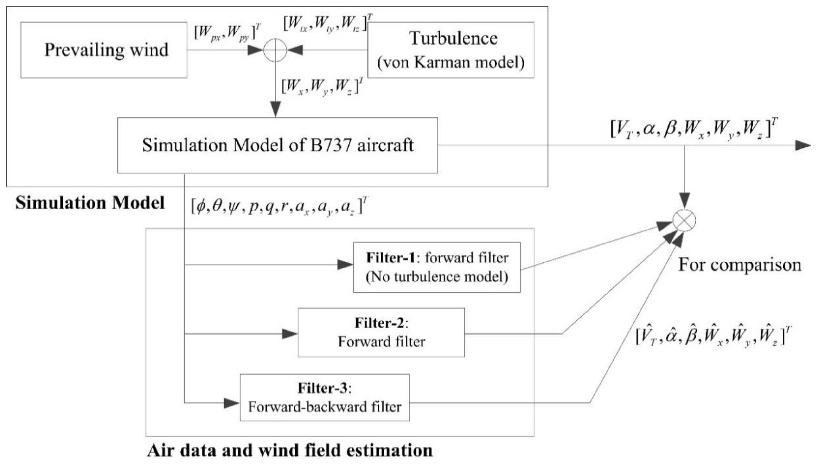
Since it is impractical to verify the method by directly comparing the estimated results to the inaccurate recorded flight data, a simulation verification scheme was designed. A blended wind field combining prevailing wind and turbulence was generated, and a simulated Boeing 737–800 aircraft was flying through the wind field, as shown in Figure 2. The simulation model of the B737–800 aircraft was built based on the aerodynamic and aero-engine performance data provided by [35,36,37]. There are three advantages to this simulation scheme. First, during the simulation, the flight parameters obtained by numerical integration can be used as inertial measurements. Second, the estimated air data and wind components can be compared with simulation results. Third, the estimated turbulence can also be compared with the theoretical turbulence model.
Four simulation conditions (SC) with different turbulence intensities and different flight states were set for algorithm verification, as shown in Table 1. Turbulence can be classified as light, moderate, or severe turbulence, depending on the turbulence intensity [29]. Level flight and turn flight scenarios were used to test the algorithm, while the latter can be further used to test the instantaneous tracking performance of different filters. Spatial turbulence based on the von Karman model was generated and integrated into the simulation model. Furthermore, the sinusoidal prevailing wind in the horizontal plane was set by
{ W p x = W sin ( 2 π T t + φ ) cos γ W p y = W sin ( 2 π T t + φ ) sin γ ,
where W is the amplitude of prevailing wind, γ , represents the wind angle relative to the aircraft. Compared to the rapid-changing turbulence, the period of prevailing wind was set by the parameter T . In this study, T was set to 120 s to describe the slowly time-varying gust wind.
Taking SC-3 as an example, after trimming the simulation model at SC-3, the simulated wind components [ W x , W y , W z ] T and inertial measurements [ a x , a y , a z , p , q , r , ϕ , θ , ψ ] T of a period of 120 s are shown in Figure 3. In moderate turbulence, the aircraft was first controlled to turn right during 20~50 s with turn rate r = 1.2 / s and sideslip angle of β = 1.2 . After that, during 60~90 s, the aircraft was controlled to turn left with r = 1.2 / s . The first subgraph shows the wind components [ W x , W y , W z ] T , which are the assembly of horizontal prevailing wind and turbulence. The second subgraph shows the simulated acceleration [ a x , a y , a z ] T along three axes. The third subgraph shows the angular rate [ p , q , r ] T , while the fourth subgraph shows the attitude angle [ ϕ , θ , ψ ] T along three axes.
Three filters were used for comparison in this study. The first filter, Filter-1, was the forward Kalman Filter in which Equations (6) and (12) were assembled as the system update equations, and the turbulence was only regarded as random noise. The second filter, Filter-2, was the forward filter with turbulence model using Equation (13) as the system update equation. The third filter, Filter-3, was the forward–backward filter proposed in Section 2.3.2.

3.1.2. Performance Comparison of Three Filters

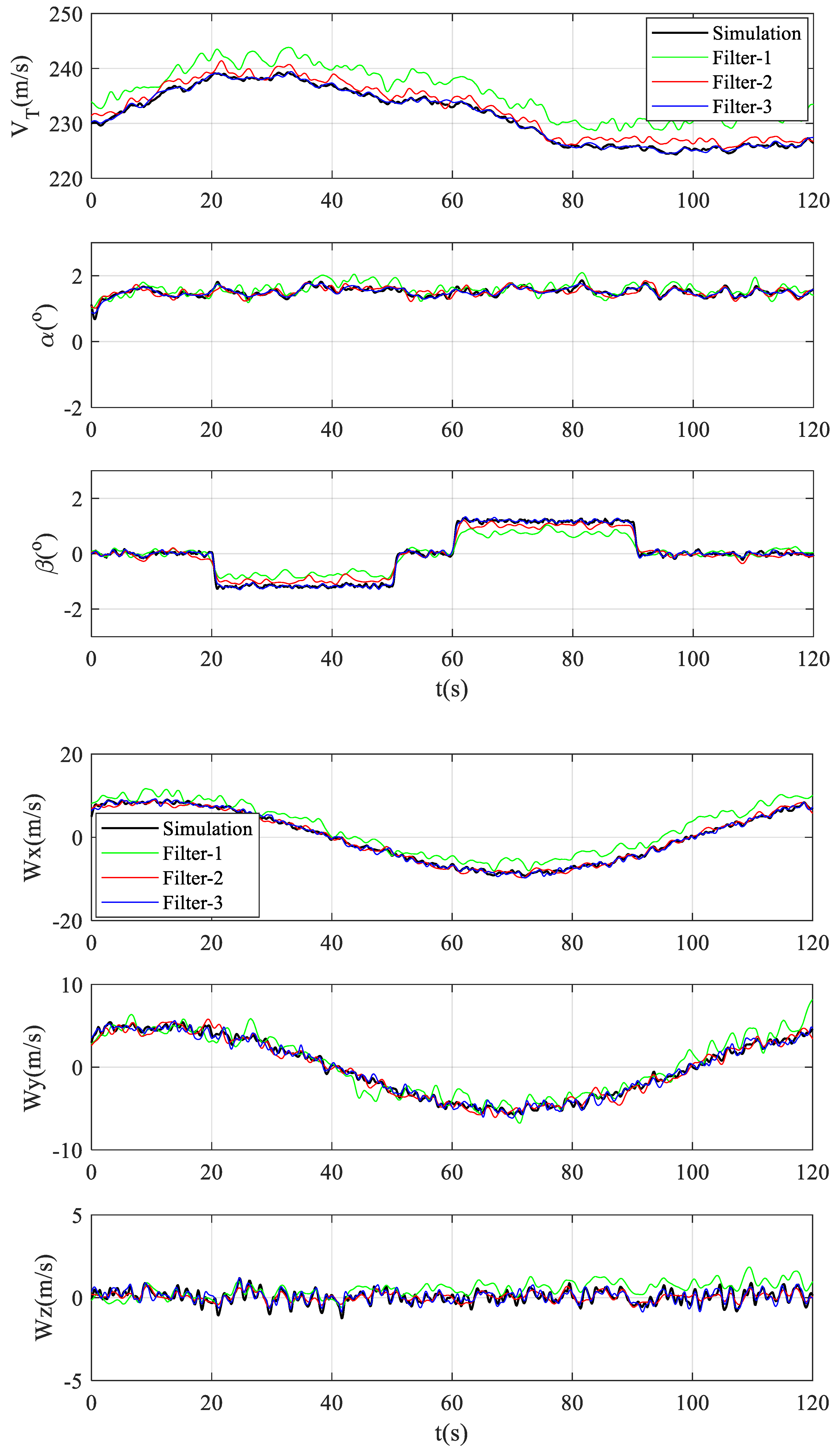
The SC-3 with turn flight maneuvers was first used to test the estimation performance of three filters. The 120-s filtering results of Filter-1, Filter-2, and Filter-3, including the air data [ V T , α , β ] T , and wind components [ W x , W y , W z ] T , are shown in Figure 4.
Based on the generated flight parameters by simulation, the initial value of air data and wind components in three filters were set in advance according to Equations (1)–(5). Benefitted by the initial value settings, three filters were able to track the simulation results within several steps. The experiments also indicate that a better initial value not only lowers the risk of divergence but also improves the convergence rate and accuracy of the filters. The air data filtering system built by inertial measurements is effective. From the tracking process, the estimation accuracy of Filter-2 and Filter-3 was much better than that of Filter-1. It shows that the integrated von Karman turbulence model can effectively reduce the tracking error. Filter-3 with forward–backward filter showed the best tracking accuracy. Furthermore, it also showed stronger instantaneous tracking ability in the tracking process of sideslip angle.
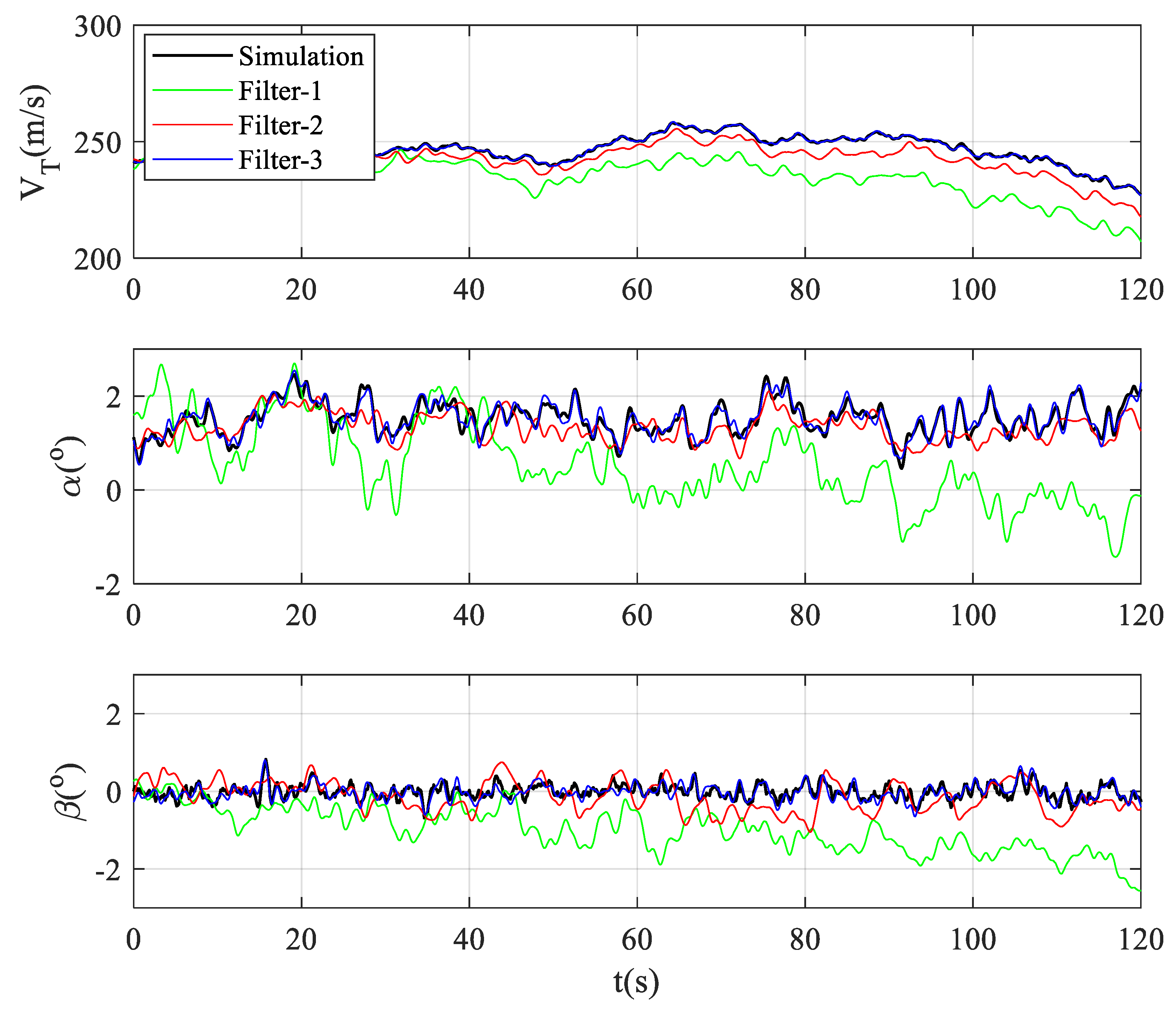
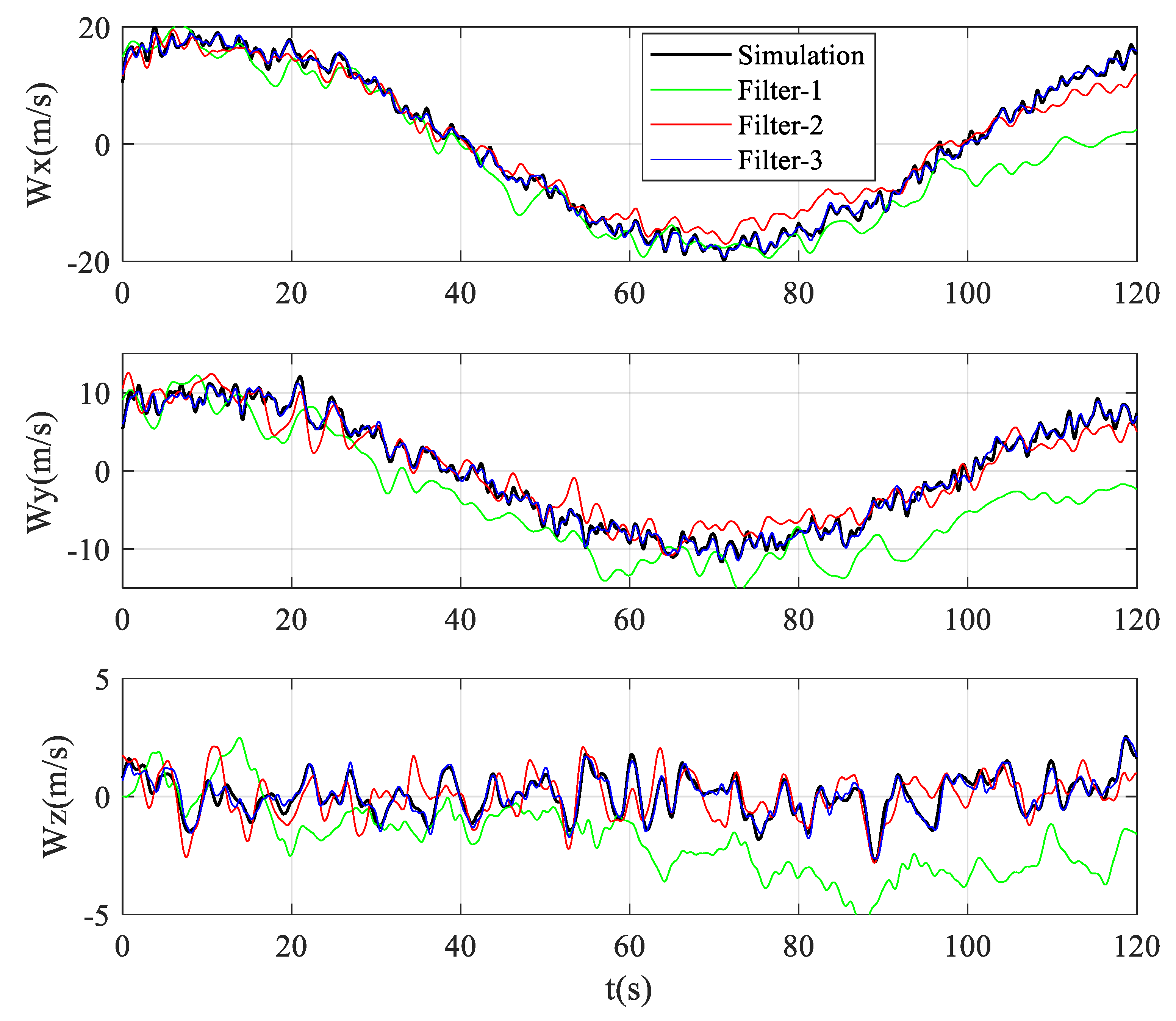
A severe turbulent flight scenario, SC-4, was used to test the performance of three filters further. As shown in Figure 5, the estimation performance of Filter-1 and Filter-2 further deteriorated. On the contrary, Filter-3 was able to track the simulation results well, and there was no instability with the increase in estimation error. Experiments showed that Filter-3 had the best convergence rate, estimation accuracy, and stability than the other two filters. When it comes to Filter-1 with random noise as the turbulence, it leads to a poor estimation accuracy in severe turbulence because the deviation of Filter-1 increases sharply. Compared to Filter-2, the backward filter in Filter-3 can effectively improve the estimation accuracy. With the standard variation of v k set as 1, the tracking error of Filter-3 can be reduced by 63.1% by backward filtering.
Here is a further analysis on the trace of the covariance matrix, t r ( P ) , which was used to describe the error change in the estimation process. Figure 6 shows the change in t r ( P ) of different standard variations of measuring noise, σ ( v k ) = 1 , σ ( v k ) = 5 and σ ( v k ) = 10 . Taking σ ( v k ) = 5 as an example, at the time t = 50 s, the trace of covariance matrix reduced to and maintained at 1.753 in Filter-2. It shows that the estimation accuracy cannot be improved further by forward filtering only. The trace of backward filter also reduced to 1.753 from initial infinity at t = 120 s. However, the final t r ( P ) at t = 70 s was reduced to 0.551 by Filter-3. In the post-process of flight data, the estimation accuracy in the fixed time interval can be effectively improved by the backward filter because more measurements are used in the filtering system. Another finding is that with the increase in σ ( v k ) , the percentage of accuracy improvement by backward filter became smaller. The reason is that if the measuring noise increases, more measurements are not helpful for the accuracy improvement. However, according to accuracy characteristics shown in Table A1, the standard variation of recorded inertial measurements is acceptable. As a result, it is an effective way for estimation accuracy improvement by backward filtering based on flight data.
One of the advantages of the simulation verification is that the estimated turbulence can also be compared to the theoretical von Karman model. Due to the randomness of turbulence, it was difficult to ensure that the filtering algorithm could estimate accurately at every time step. However, the statistical characteristics of estimated turbulence can be obtained from a large number of filtering results. If the statistical characteristics of the estimated turbulence approach that of the turbulence model, it can be concluded that the estimated turbulence is credible.
An analysis was conducted on the frequency content of three turbulence components. To obtain the spectral density of the estimated turbulence, the Welch spectrum density estimation with the Hamming window was adopted based on a long time series of turbulence components [38]. The data length in the time-domain for each curve was 2560 points, representing a length of 640 s turbulence component. With the sampled turbulence components at 4 Hz, the window length was 10 × fs = 40, and the overlapping was set to 50%.
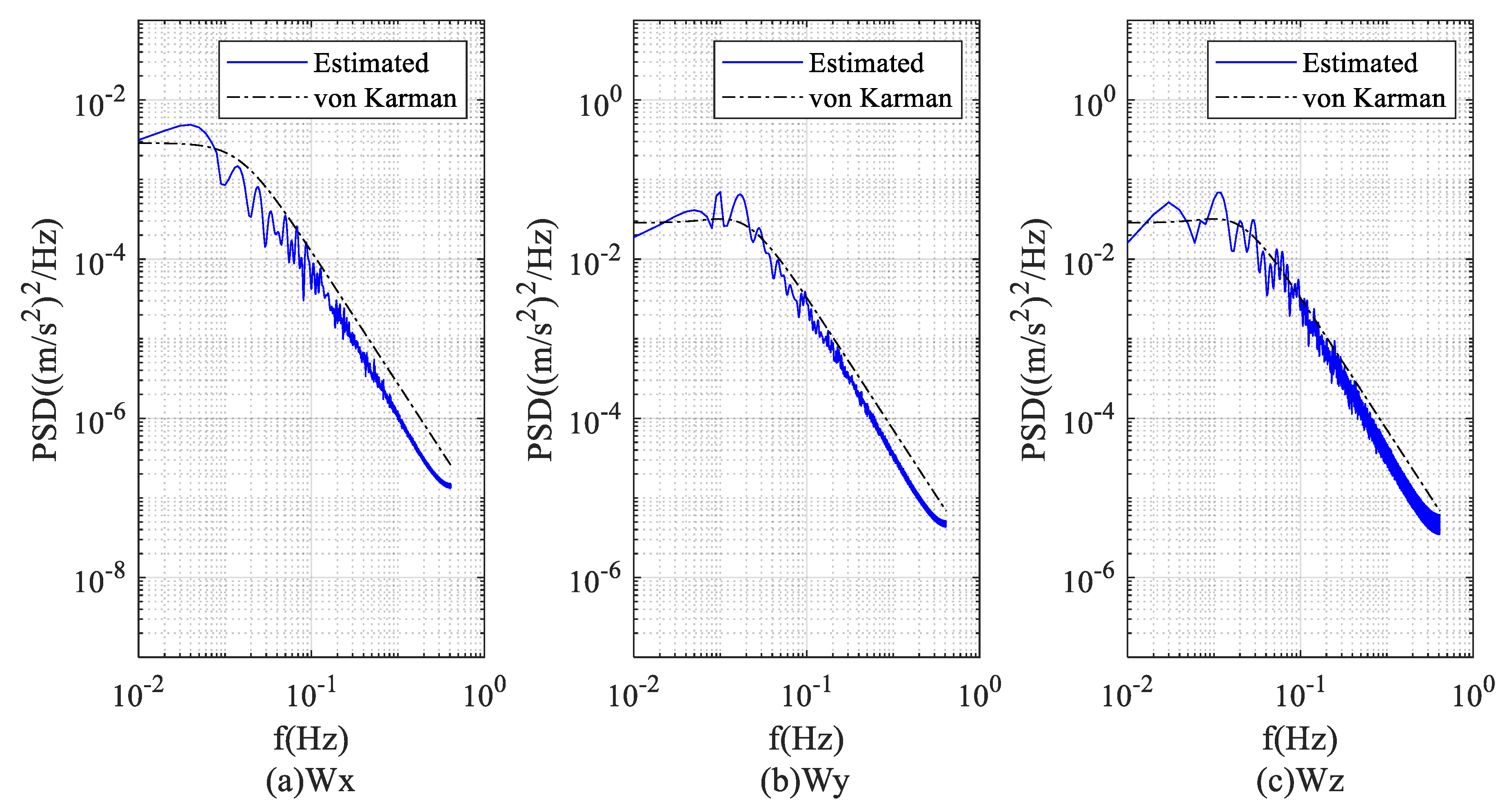
Taking SC-2 as an example, Figure 7 indicates that the spectra of estimated turbulence components by Filter-3 were consistent with that of the theoretical model. Especially in the high-frequency section, the estimation results had a gradual property with a slope of −5/3, which conforms to Kolmogorov turbulence theory. On the contrary, without the turbulence model, Filter-1 did not have similar results as the theoretical model. Results showed that the estimated turbulence is credible in a statistical sense. The estimation results, as shown in Figure 4 and Figure 5, also indicate that the integration of the von Karman model improves the estimation accuracy remarkably.
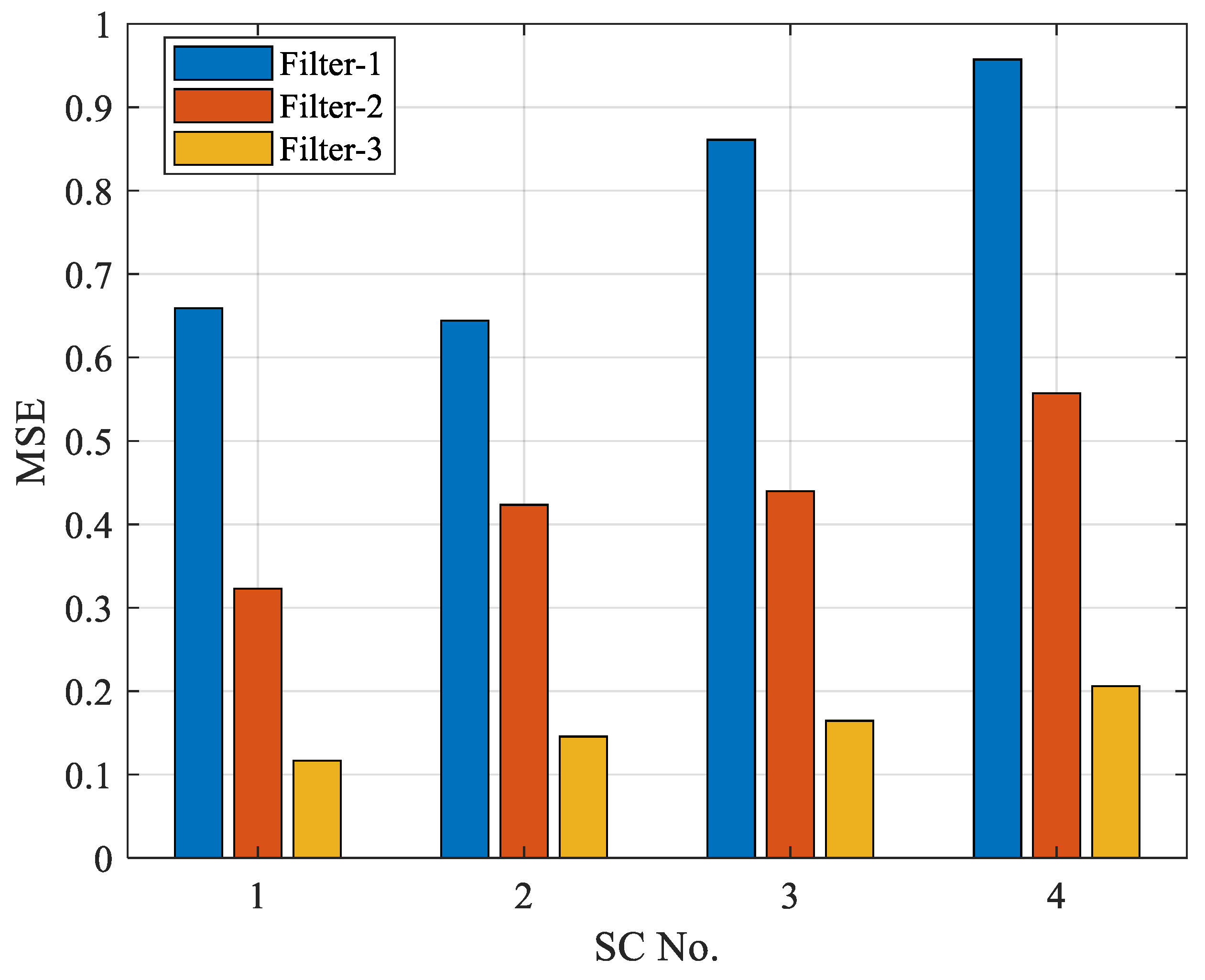
The influence of different turbulence intensities on three filters was further analyzed. After standardizing six state parameters, a statistical analysis of the mean square estimation error (MSE) after convergence was conducted on the four SCs, as shown in Figure 8. Benefitted by the von Karman turbulence model and backward filtering, Filter-3 had the best estimation performance. With the increase in turbulence intensity, the estimation error of Filter-3 scarcely changed. In addition, compared with SC-2, turn flight maneuver (in SC-3) had few effects on the accuracy and stability of Filter-3.
With this simulation scheme, the proposed method was verified by simulation. It was difficult to build the aerodynamic and aero-engine model with enough accuracy in wind disturbance. However, the proposed filtering system with inertial measurements was capable of estimating wind-affected air data and wind field. In particular, the integration of the von Karman turbulence model can effectively reduce the tracking error and assured filtering stability. Furthermore, the forward–backward filtering algorithm can further improve the filtering accuracy.

3.2. Experiments with Flight Data

This section uses the Quick Access Recorder (QAR) flight data for the test. Supported by Chinese airlines, the flight data were gathered from the B737–800 aircraft on the same scheduled air route. The time series of flight data contained related parameters for filtering but with different sampling rates and resolutions.

3.2.1. In-Turbulence Air Data and Wind Field Estimation

The forward–backward filtering was carried out in this section based on actual flight data. Because of the different sampling rates of required flight data shown in Table A1, the measurement and system update operations could not be executed simultaneously. Unequal interval filtering is commonly used to solve this problem [28]. Taking the forward filter as an example, if there were no measurements output at this moment because of low sampling rate, only the system update was executed as
{ x ^ f k = F k 1 x ^ f , k 1 + P f k = F k 1 P f , k 1 + F k 1 T + Q k 1 .
Once there were measurements output, the system and measurement update were executed simultaneously as
{ K f k = P f k H k T ( H k P f k H k T + R k ) 1 x ^ f k + = x ^ f k + K f k ( y k H k x ^ f k ) P f k + = ( I K f k H k ) P f k .
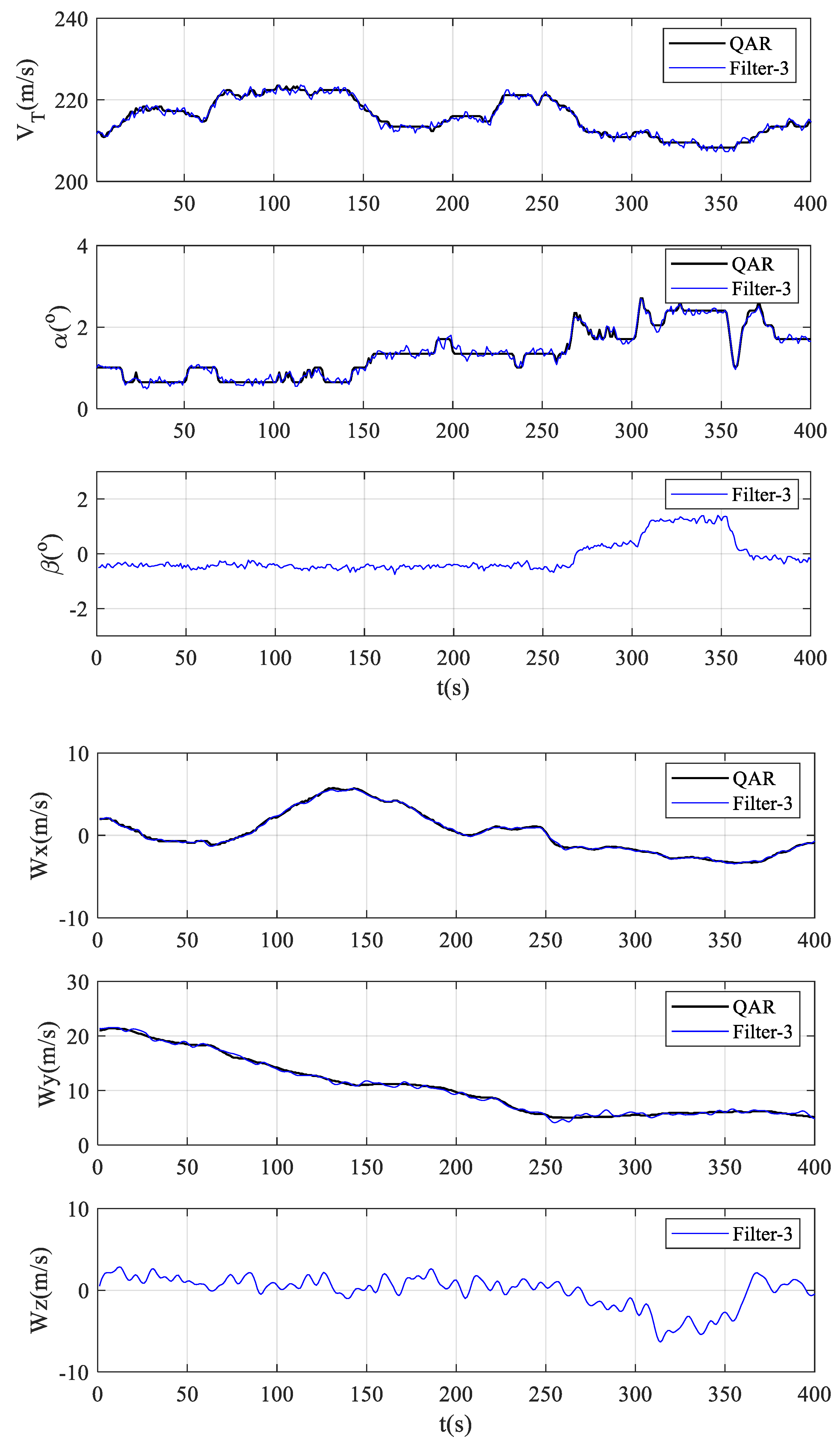
The filtering results of Filter-3 based on a time series of flight data in severe turbulence are shown in Figure 9, in which the trend of estimated air data and wind field approximates the derived value from recorded fight data. In turbulent flight, the ADS onboard the aircraft cannot respond to the rapid change in wind disturbance, which makes the recorded airspeed and angle of attack show the characteristics of low-pass filtering. However, the instantaneous change in air data can be estimated by Filter-3. In addition, compared to the assumption of sinusoidal prevailing wind in Section 3.1, the actual wind field was irregular. With the exponentially-correlated wind model integrated, Filter-3 was able to track the change in prevailing wind in a wide range.

3.2.2. Effects of Uncertain Disturbance on Filtering

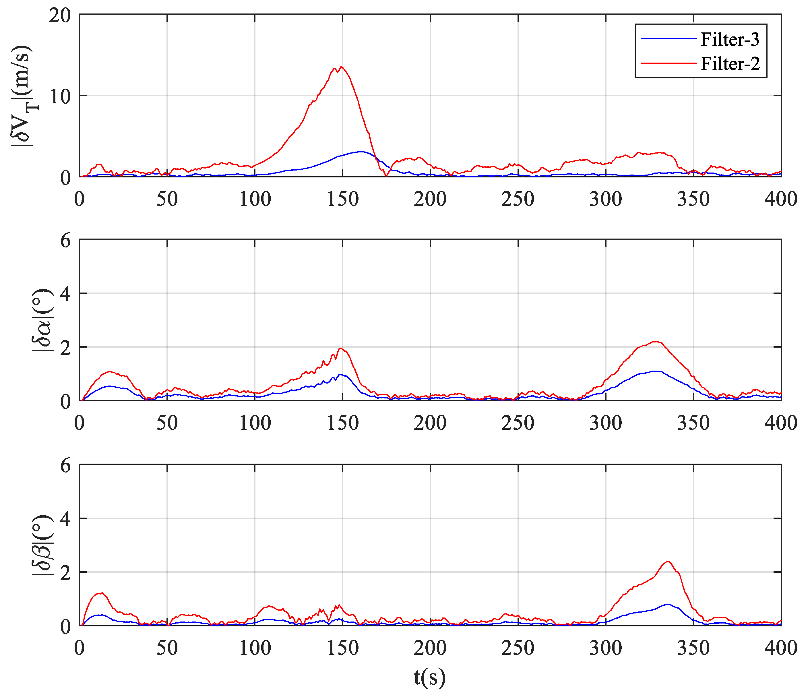
In the collecting and transmitting procedure, the flight data may easily be disturbed, leading to serious deviations of the recorded value. Thus there inevitably exists uncertain disturbance in flight data. A time series of abnormal flight data shows that a sudden external disturbance occurred on the acceleration measurements at 100~150 s, resulting in a serious deviation from the real value. At 300~320 s, there was a non-zero noise with greater covariance that affected the measurements of angular rate. Under the unexpected disturbance, all three filters lack fault tolerance. Figure 10 shows the comparison of estimated results of Filter-2 and Filter-3.
Compared to Filter-2 without backward filtering, the estimation error of Filter-3 was reduced. In backward filtering, more measurements make the estimation procedure smoother, which is also helpful to reduce the estimation error caused by sudden disturbance. As a result, the forward–backward filter had better stability and adaptability to deal with uncertain disturbances in flight data.
The proposed filtering method showed its practicability from the test with actual flight data. The instantaneous change in air data and wind components can be estimated by the proposed method, which is fundamental to obtaining the accurate aerodynamic performance of aircraft in adverse wind effects. Moreover, in response to a sudden disturbance, the backward filter can effectively reduce the estimation error by using more measurements.

4. Conclusions

To obtain air data and wind field with better accuracy is fundamental to obtaining accurate aerodynamic performance, thus assisting flight quality and accident analysis of civil aviation aircraft. This paper put forward a new in-turbulence air data and wind field estimation method based on flight data. Some innovations are as follows:
(1) A new filtering system was built to estimate the air data and wind field. The inertial measurements, insensitive to wind disturbance, were used to build the system update equation. With the recorded inertial measurements, it is no longer necessary to build an accurate aerodynamic and aero-engine model in wind disturbance.
(2) To better describe the wind field characteristics in high-altitude, the exponentially correlated stochastic model and von Karman turbulence model were integrated into the filtering system to describe the horizontal prevailing wind and turbulence, respectively.
(3) Benefitted by the post-processing characteristics of flight data, a forward–backward filtering algorithm was designed, in which the backward filter is capable of improving the estimation accuracy further.
The simulation shows that the proposed filtering system can not only ensure stability but also reduce the estimation error effectively. By backward filtering, the estimation error is reduced with the increase in measurements. Experiments with real QAR data showed that the instantaneous change in air data and wind components could be estimated. For the fixed-length time series of flight data, the forward–backward filter can be used to reduce the adverse effects of uncertain disturbance on air data and wind field estimation.
This study is the first attempt to apply forward–backward filtering to process flight data. One potential weakness of this study is that the noises of inertial measurements were assumed to follow a normal distribution. However, the actual noise model of flight data is uncertain. Some extended filtering algorithms should be developed to solve this problem. Furthermore, different turbulence models describing the intermittent wind fluctuation need to be developed and integrated into the filtering system.

Author Contributions

Conceptualization, Z.G.; methodology, Z.G. and H.W.; software, D.W. and Z.X.; validation, Z.G., H.W.; formal analysis, Z.G.; investigation, H.W.; resources, D.W.; data curation, Z.X.; writing—original draft preparation, Z.G.; writing—review and editing, H.W. and Z.X.; visualization, D.W.; supervision, Z.G.; project administration, Z.G.; funding acquisition, Z.G. All authors have read and agreed to the published version of the manuscript.

Funding

This research was funded by the Natural Science Foundation of China, grant number [NSFC: U1733122].

Institutional Review Board Statement

Not applicable.

Informed Consent Statement

Not applicable.

Data Availability Statement

Exclude.

Conflicts of Interest

The authors declare no conflict of interest.

Appendix A

According to “Digital flight data acquisition unit 737-600/-700/-700C/-800/-900 data frame interface control and requirements document”, the characteristics of related parameters in this paper are listed as follows.
Table A1. Characteristics of recorded parameters.
Parameter TypeParameter AssignmentSymbol (Unit)Sampling Rate/HzOut ResolutionOut RangeAccuracy
Inertial measurementsLongitudinal acceleration a x   ( g ) 40.000976563−1~+10.01
Lateral acceleration a y   ( g ) 40.00203649−1~+10.01
Vertical acceleration a z   ( g ) 80.001953125−3~60.046
Roll angle ϕ   ( ) 40.005493164−90~900.05
Pitch angle θ   ( ) 40.005493164−90~900.05
Yaw angle ψ   ( ) 20.005493164−180~1800.05
Roll angular rate p   ( / s ) 80.00390625−45~450.1
Pitch angular rate q   ( / s ) 80.00390625−45~450.1
Yaw angular rate r   ( / s ) 80.00390625−45~450.1
Ground speed V G   ( k n o t ) 40.10~1024N/A
Air dataMach number M 10.0010~1.024N/A
Angle of attack α ¯   ( ) 10.17578125−90~90N/A
Total temperature t   ( ° C ) 10.5−512~512N/A

References

  1. Burns, A.A.; Chenkovich, G.A. Digital Flight Data Acquisition Unit 737-600/-700/-700C/-800/-900 Data Frame Interface Control and Requirements Document; Report. No. D226A101-2; The Boeing Company: Seattle, WA, USA, 2003. [Google Scholar]
  2. Sharman, R.D.; Lane, T. Aviation Turbulence: Processes, Detection, Prediction; Springer: Cham, Switzerland, 2016. [Google Scholar]
  3. Sikkel, L.N.C.; Croon, G.C.H.E.; Wagter, C.D.; Chu, Q.P. A novel online model-based wind estimation approach for quadrotor micro air vehicles using low cost MEMS IMUs. In Proceedings of the 2016 IEEE/RSJ International Conference on Intelligent Robots and Systems (IROS), Daejeon, Korea, 9–14 October 2016; pp. 2141–2146. [Google Scholar]
  4. Li, R.; Lu, C.; Liu, J.; Lei, T. Air data estimation algorithm under unknown wind based on information fusion. J. Aerosp. Eng. 2018, 31, 040418072. [Google Scholar] [CrossRef]
  5. Colgren, R.D.; Frye, M.T.; Olson, W.M. A proposed system architecture for estimation of angle of attack and sideslip angle. In Proceedings of the AIAA Guidance, Navigation, and Control Conference and Exhibit, Portland, OR, USA, 9–11 August 1999. [Google Scholar]
  6. Myschik, S.; Holzapfel, F.; Sachs, G. Low-cost sensor based integrated air data and navigation system for general aviation aircraft. In Proceedings of the AIAA Guidance, Navigation, and Control Conference and Exhibit, Honolulu, HI, USA, 18–21 August 2008. [Google Scholar]
  7. Wise, K.A. Flight testing of the X-45A J-UCAS computational alpha-beta system. In Proceedings of the AIAA Guidance, Navigation, and Control Conference and Exhibit, Keystone, CO, USA, 21–24 August 2006. [Google Scholar]
  8. Cho, A.; Kim, J.; Lee, S.; Kee, C. Wind estimation and airspeed calibration using a UAV with a single-antenna GPS receiver and Pitot tube. IEEE Trans. Aerosp. Electron. Syst. 2011, 47, 109–117. [Google Scholar] [CrossRef]
  9. Larrabee, T.; Chao, H.; Rhudy, M.; Gu, Y.; Napolitano, M.R. Wind field estimation in UAV formation flight. In Proceedings of the American Control Conference, Portland, OR, USA, 4–6 June 2014; pp. 5408–5413. [Google Scholar]
  10. Lie, F.A.P.; Egziabher, D.G. Synthetic air data system. J. Aircr. 2013, 50, 1234–1249. [Google Scholar] [CrossRef]
  11. Nebula, F.; Palumbo, R.; Morani, G. Virtual air data: A fault-tolerant approach against ADS failures. In Proceedings of the AIAA Infotech at Aerospace Conference, Boston, MA, USA, 19–22 August 2013. [Google Scholar]
  12. Lv, P.; Lai, J.; Liu, J.; Zhu, B.; Song, Y. Overview and progress on study of aircraft aerodynamics model aided navigation method. Control Decis. 2015, 30, 2113–2120. [Google Scholar]
  13. Karlgaard, C.D.; Kutty, P.; Schoenenberger, M. Coupled inertial navigation and flush air data sensing algorithm for atmosphere estimation. J. Spacecr. Rocket. 2017, 54, 128–140. [Google Scholar] [CrossRef]
  14. Johansen, T.A.; Cristofaro, A.; Sorensen, K.; Hansen, J.M.; Fossen, T.I. On estimation of wind velocity, angle of attack and sideslip angle of small UAVs using standard sensors. In Proceedings of the International Conference on Unmanned Aircraft Systems (ICUAS), Denver, CO, USA, 23–25 November 2015; pp. 510–519. [Google Scholar]
  15. Lee, J.H.; Sevil, H.E.; Dogan, A.; Hullender, D. Estimation of maneuvering aircraft states and time-varying wind with turbulence. In Proceedings of the AIAA Guidance, Navigation and Control Conference, Minneapolis, MN, USA, 13–16 August 2012. [Google Scholar]
  16. Grillo, C.; Montano, F. Wind component estimation for UAS flying in turbulent air. Aerosp. Sci. Technol. 2019, 93, 1–7. [Google Scholar] [CrossRef]
  17. Mutlu, T.; Hajiyev, C. An integrated air data/GPS navigation system for helicopters. Positioning 2011, 2, 103–111. [Google Scholar] [CrossRef] [Green Version]
  18. Guo, D.; Zhong, M.; Zhou, D. Multi sensor data-fusion-based approach to airspeed measurement fault detection for unmanned aerial vehicles. IEEE Trans. Instrum. Meas. 2018, 67, 317–327. [Google Scholar] [CrossRef]
  19. Rhudy, M.B.; Gu, Y.; Gross, J.N.; Chao, H. Onboard wind velocity estimation comparison for unmanned aircraft systems. IEEE Trans. Aerosp. Electron. Syst. 2017, 53, 55–66. [Google Scholar] [CrossRef]
  20. Hajiyev, C.; Guler, D.C.; Hacizade, U. Two-stage Kalman filter for estimation of wind speed and UAV flight parameters based on GPS/INS and pitot tube measurements. In Proceedings of the 9th International Conference on Recent Advances in Space Technologies (RAST), Istanbul, Turkey, 11–14 June 2019; pp. 875–880. [Google Scholar]
  21. Rhudy, M.B.; Fraolini, M.L.; Porcacchia, M.; Napolitano, M.R. Comparison of wind speed models within a Pitot-free airspeed estimation algorithm using light aviation data. Aerosp. Sci. Technol. 2019, 86, 21–29. [Google Scholar] [CrossRef]
  22. Sun, K.; Regan, C.D.; Egziabher, D.G. GNSS/INS based estimation of air data and wind vector using flight maneuvers. In Proceedings of the IEEE/ION Position, Location and Navigation Symposium (PLANS), Monterey, CA, USA, 23–26 April 2018; pp. 838–849. [Google Scholar]
  23. Gao, Z.; Wang, H.; Qi, K.; Xiang, Z.; Wang, D. Acceleration-based in situ eddy dissipation rate estimation with flight data. Atmosphere 2020, 11, 1247. [Google Scholar] [CrossRef]
  24. Wenz, A.; Johansen, T.A. Moving horizon estimation of air data parameters for UAVs. IEEE Trans. Aerosp. Electron. Syst. 2020, 56, 2101–2121. [Google Scholar] [CrossRef] [Green Version]
  25. Tian, P.; Chao, H.; Gu, Y.; Hagerott, S.G. UAV flight test evaluation of fusion algorithms for estimation of angle of attack and sideslip angle. In Proceedings of the AIAA Guidance, Navigation, and Control Conference, San Diego, CA, USA, 4–8 January 2016. [Google Scholar]
  26. Tian, P.; Chao, H. Model aided estimation of angle of attack, sideslip angle, and 3D wind without flow angle measurements. In Proceedings of the AIAA Guidance, Navigation, and Control Conference, Kissimmee, FL, USA, 8–12 January 2018. [Google Scholar]
  27. Wang, Y.; Keviczky, T. Real-time fault-tolerant moving horizon air data estimation for the reconfigure benchmark. IEEE Trans. Control Syst. Technol. 2019, 27, 997–1011. [Google Scholar]
  28. Simon, D. Optimal State Estimation: Kalman, H Infinity and Nonlinear Approaches; Wiley: Hoboken, NJ, USA, 2006. [Google Scholar]
  29. Wright Patterson Air Force Base. Flying Qualities of Piloted Airplanes, MIL-F-8785C; U.S. Air Force: Dayton, OH, USA, 1980.
  30. Duran, I.B.; Schmidli, J.; Bhattacharya, R. A budget-based turbulence length scale diagnostic. Atmosphere 2020, 11, 425. [Google Scholar] [CrossRef] [Green Version]
  31. Rabbath, C.A.; Lechevin, N. Discrete-Time Control System Design with Application; Springer: New York, NY, USA, 2014. [Google Scholar]
  32. Stevens, B.L. Aircraft Control and Simulation, 3rd ed.; Wiley: New York, NY, USA, 2015. [Google Scholar]
  33. Ienkaran, A.; Simon, H. Cubature Kalman smoothers. Automatica 2011, 47, 2245–2250. [Google Scholar]
  34. Pnevmatikakis, E.A.; Rad, K.R.; Huggins, J.; Paninski, L. Fast Kalman filtering and forward–backward smoothing via a low-rank perturbative approach. J. Comput. Graph. Stat. 2014, 23, 316–339. [Google Scholar] [CrossRef]
  35. Ernst, D.O.; Grammens, D. CFM56-7 Propulsion System Data for the 737-600/-700/-800 Training Simulator; Report No. D611A025; The Boeing Company: Seattle, WA, USA, 2005. [Google Scholar]
  36. Jens, D.R.; Neville, K.W.; Draxler, J.G. Aerodynamic Data and Flight Control System Description for the 737-600/-700/-800/-900 Training Simulator; Report No. D611A001-VOL1; The Boeing Company: Seattle, WA, USA, 2003. [Google Scholar]
  37. Shikany, D.A.; Neville, K.W.; Harrington, T.A. Aerodynamic Data for the 737-800 Training Simulator; Report No. D611A001-VOL3; The Boeing Company: Seattle, WA, USA, 2003. [Google Scholar]
  38. Stoica, P.; Moses, R. Spectral Analysis of Signals; Pearson Education: Cranbury, NJ, USA, 2005. [Google Scholar]
Figure 1. Forward–backward filtering.
Atmosphere 12 00470 g001
Figure 2. The simulation verification process.
Atmosphere 12 00470 g002
Figure 3. Simulated wind field and inertial measurements in simulation conditions 3 (SC-3).
Atmosphere 12 00470 g003
Figure 4. Air data and wind field estimation in SC-3.
Atmosphere 12 00470 g004
Figure 5. Air data and wind field estimation in SC-4.
Atmosphere 12 00470 g005aAtmosphere 12 00470 g005b
Figure 6. The change in the trace of the covariance matrix.
Atmosphere 12 00470 g006
Figure 7. Spectrum analysis of theoretical model and estimated turbulence. (a) Estimated and theoretical spectra of Wx. (b) Estimated and theoretical spectra of Wy. (c) Estimated and theoretical spectra of Wz.
Atmosphere 12 00470 g007
Figure 8. Mean square estimation error (MSE) of estimation results under different SCs.
Atmosphere 12 00470 g008
Figure 9. Air data and wind field estimation based on Quick Access Recorder (QAR) flight data.
Atmosphere 12 00470 g009
Figure 10. The convergence performance in uncertain disturbances.
Atmosphere 12 00470 g010
Table 1. Simulation conditions (SC).
Simulation
Condition
Prevailing WindTurbulence
Intensity
Flight State
SC-1 W = 5   m / s , γ = 0 , φ = 0 Light, σ = 0.5   m / s Level flight, h = 8000   m , M = 0.74
SC-2 W = 10   m / s , γ = 30 , φ = 30 Moderate, σ = 2   m / s Level flight, h = 10,000   m , M = 0.76
SC-3 W = 10   m / s , γ = 30 , φ = 30 Moderate, σ = 1.5   m / s Turn flight, h = 10,000   m , M = 0.76 , r = 1.2 / s
SC-4 W = 20   m / s , γ = 30 , φ = 60 Severe, σ = 5   m / s Level flight, h = 12,000   m , M = 0.78
Publisher’s Note: MDPI stays neutral with regard to jurisdictional claims in published maps and institutional affiliations.