Article

Estimation of the Latent Heat Flux over Irrigated Short Fescue Grass for Different Fetches

by
Francesc Castellví
1,* and
Pedro Gavilán
2
1
Department Medi Ambient i Cienciès del Sòl, University of Lleida, E.T.S.E.A, Rovira Roure 191, 25198 Lleida, Spain
2
Instituto de Investigación y Formación Agraria y Pesquera, Área de Agricultura y Medio Ambiente, Centro Alameda del Obispo, Avda. Menéndez Pidal s/n, 14004 Córdoba, Spain
*
Author to whom correspondence should be addressed.
Atmosphere 2021, 12(3), 322; https://doi.org/10.3390/atmos12030322
Submission received: 29 December 2020 / Revised: 21 February 2021 / Accepted: 23 February 2021 / Published: 1 March 2021
(This article belongs to the Special Issue Agricultural Microclimate and Irrigation Water Management)

Abstract

:
Often in agrometeorology the instrumentation required to estimate turbulent surface fluxes must be installed at sites where fetch is not sufficient for a sector of wind directions. For different integrated flux-footprints (IFFP) thresholds and taking as a reference the half-hourly latent heat fluxes (LE) measured with a large weighing lysimeter (LELys), the eddy covariance (EC) method and two methods based on surface renewal (SR) analysis to estimate LE were tested over short fescue grass. One method combined SR with the flux-gradient (profile) relationship, SR-P method, and the other with the dissipation method, SR-D method. When LE was estimated using traces of air moisture, good performances were obtained using the EC and the SR-P methods for samples with IFFP higher than 85%. However, the closest LE estimates were obtained using the residual method. For IFFP higher than 50%, the residual method combined with the sensible heat flux estimates determined using the SR-P method performed close to LELys and using the SR-D method good estimates were obtained for accumulated LELys. To estimate the sensible heat flux, the SR-D method can be recommended for day-to-day use by farmers because it is friendly and affordable.

1. Introduction

Evapotranspiration, or latent heat flux (LE), is required as input to improve weather forecasting, fire index, irrigation, dynamics of ecosystems and many other applications. In agriculture, most of the complexity to estimate LE is greatly reduced in lands where homogeneous crops grow in an open and flat terrain scenario [1,2,3]. Two crucial simplifications to estimate LE for such scenario are the following. First, the simplified surface energy balance equation holds. That is, the net radiation, Rn, minus ground heat flux, G, often is close to the sum of sensible heat, H, and LE; (Rn − G) = (H + LE). This equation is involved in different methods to estimate LE, such as in the Penman-Monteith equation, the Bowen ratio-surface energy balance method and the residual method [1,4,5,6,7,8,9,10]. Second, measurements can be taken in the inertial sublayer (i.e., it is not required to install tall masts) where the Monin–Obukhov Similarity Theory (MOST) relationships hold. As a rule of thumb, the basis of the inertial sublayer is estimated as at least two times the canopy height and crucial canopy parameters involved in MOST relationships, such as the zero-plane displacement and the aerodynamic roughness lengths for momentum and heat, may be estimated as a proportion of the canopy height [1,2,11,12].
Unfortunately, the latter scenario is rarely met. Often, crops grow in small plots which may be surrounded by different crops, drier fields or bare soils. From a micrometeorological point of view, small plot refers to a surface which dimensions may compromise the method used to estimate LE. Measurements must be taken within the internal surface boundary layer, and the gold rule used as a guide in the field is to deploy the instrumentation at the (measurement height):(fetch distance) ratio of 1:100 at neutral conditions. Higher and lower ratios are required for stable and unstable cases, respectively [1,13,14]. In a small plot scenario, the inertial sublayer may be thin and variable which makes difficult to decide the measurement height. Under such scenario, methods requiring measurements at one height are preferred. However, depending on the method used, other issues must be considered. For instance, to apply the eddy covariance (EC) method it is recommended to deploy the sonic anemometer at a height of at least 18 times the instrument path length. The latter is required to sample eddy sizes much larger than the measuring path length and to avoid weak mean vertical velocity fluctuations [15]. Thus, for short grass (e.g., 10 cm tall) the sonic anemometer should operate at a height higher than 2 m and 4 m when its path length is of about 12 cm and 20 cm, respectively [5]. The latter requires plots with a minimum radius of about 200 (400) m around the measurement point. Apparently, a large weighing lysimeter bypasses such issue. In any case, latent heat flux measurements made using both weighing lysimeters and the EC method (both established as a reference to determine the latent heat flux [1,16]) are expensive. In fact, their acquisition and maintenance only can be justified for research purposes, and data post-processing requires personnel with skills in micrometeorology [17,18,19]. In practice, affordable methods to estimate LE are of interest, and the small plot issue is rather common. The small plot scenario is not restricted to small farms. Even in large fields, the instrumentation often must be deployed at sites where power, safety and surveillance can be guaranteed. Research facilities are not exempt of the small plot issue because maintenance of experimental plots accomplishing fetch requirements is expensive, and, in general, the land available to carry out different experiments is limited.
This study centers on the estimation of the latent heat flux of a short crop in a small plot scenario. The aim was to figure out if some recommendation can be given to estimate LE when the fetch is not sufficient in a sector of the field. The LE measured with a weighing lysimeter was used as a reference to compare the performance of three methods. One was the EC method which was applied deploying the instrumentation below the recommended rule (i.e., 18 times the instrument path length) to avoid, as much as possible, measurements taken above the internal boundary layer [20,21]. The other two methods combined MOST and surface renewal (SR) analysis formulation [22,23]. SR analysis for estimating the surface flux of a scalar is described in the Appendix A and the two SR-MOST methods (described in Section 2.1 and Section 2.2) were selected for two reasons: first, because they do not require calibration, and second, because their input requirements are different. One involved the flux-gradient relationship (used to describe the mean profile of a scalar), SR-P method. This requires the temperature of the air measured at high frequency and the mean wind speed as input. The other, involved the MOST relationship for the dissipation method, SR-D method. It requires traces of the temperature of the air as input. The three methods were also used to estimate the sensible heat flux to apply the residual method; LE = (Rn − G − H). Given that a net radiometer is affordable and that the soil heat flux for homogeneous canopies may be estimated as a portion of the net radiation [1], the residual method has been widely used either for assessment of LE at local and regional scales [24,25,26,27]. It is worth clarifying that this study mainly focused on the performance of the SR-MOST methods because they are more affordable than the EC method. It allows increasing the density of LE monitoring which is crucial to refine or validate methods and strategies for irrigation.

2. Theory

The kinetic surface flux of a scalar (s), w s ¯ where w is the vertical wind speed, prime denote fluctuations around the mean (Reynolds decomposition) and overbar denotes time averaging (typically half hour), is measured with the EC method [11,16]. In the framework of MOST the kinetic surface flux of a scalar is commonly expressed as, w s ¯ = u * s * , where u * and s * are the friction velocity and a scalar surface scale, respectively. It is convenient because the friction velocity can be estimated through the wind log-law [11]. Thus, the sensible heat flux, H = ρ C p   ( w T ¯ ) , where ρ is the density of the air and Cp is the isobaric specific heat capacity of the air, and the latent heat flux, LE = L   ( w ρ v ¯ ) , where L is heat of vaporization and ρ v is the water vapor density, can be rewritten as H = ρ C p u * T * and LE = L   u * ρ v * . The SR-P and SR-D methods to estimate u * s * when the measurement height is in the inertial sublayer are described next (Section 2.1 and Section 2.2, respectively) and a background on SR analysis is given in the Appendix A. Because this study focuses on the performance of the SR-P and SR-D methods, in the following the sensible heat and latent heat fluxes were determined in half-hourly basis in according to the derivation of MOST-based similarity relationships [28].

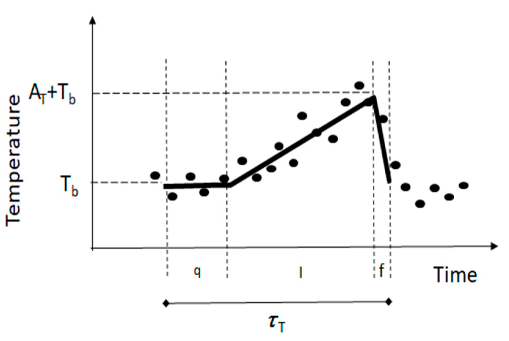
2.1. The SR-P Method

SR theory [29] in conjunction with the analysis of the scalar trace to determine the mean ramp dimensions (amplitude and period) associated to a coherent motion [30,31] can be combined with flux-gradient relationships to estimate u * s * as [22,32] (see Appendix A)
u * s * = ( k z u * π h 1 ( ε ) ) 1 / 2 A s τ s 1 / 2
where k is the von Kármán constant, z is the measurement height (Z) above the zero-plane displacement (d), ζ is the stability parameter ζ = z/L0 where L0 is the Obukhov length defined as L 0 = u * 2 k g T * T (T and g are the temperature of the air (virtual) expressed in Kelvin and acceleration due to gravity, respectively), h ( ε ) is the flux-gradient stability function for heat transfer [33], h ( ε ) = { 1 + 5 ε               0 ε 1 ( 1 16 ε ) 1 / 2 2 ε 0 , and As and τs are the amplitude and period, respectively, of the mean ramp dimensions observed in the half-hourly trace of the scalar (typically, measured at 10–20 Hz). For traces of the temperature of the air, the ramp amplitude and ε has opposite sign (see Appendix A). The friction velocity may be estimated through the wind log-law which expresses the friction velocity ( u * W P where the index WP denotes wind profile) as [1]
u * W P = k   u ln ( z z 0 m ) Ψ ( z L ) + Ψ ( z 0 m L )
where u is the mean wind speed, z0m is the roughness length for momentum and Ψ   is the integrated Businger–Dyer relationship for momentum to correct for buoyancy,
Ψ = { ln ( 0.5 ( 1 + x ) ) 2 + ln ( 0.5 ( 1 + x 2 ) ) 2 tan 1 x + 0.5 π   ξ 0 5 ξ   ξ > 0   being   x = ( 1 16 ξ ) 1 / 4

2.2. The SR-D Method

For steady and horizontally homogeneous flow, the budget equation for 0.5 s 2 ¯ with negligible local source (sink) is [11]
( w s ¯ ) s z 1 2 ( w s 2 ¯ ) z = ϵ s
The first term on the left-hand side of Equation (3) represents the production rate of 0.5 s 2 associated with turbulent motions occurring within a mean scalar gradient. The second term represents the mean turbulent transport and ϵ s , namely mean dissipation rate, represents molecular dissipation of the scalar variance. For simplicity, the transport was neglected [1,28,34]; however, it can not necessarily be small either for stable [35,36] and unstable cases [37,38,39,40,41,42,43]. Therefore, given that it is difficult to relate w s ¯ and ϵ s through Equation (3), an original dimensional analysis involving z, the turbulent standard deviation of s, σs, w s ¯ and ϵ s was proposed to relate w s ¯ and ( z ϵ s /σs). The following dissipation, D, method was proposed [42], u * s * = k D z ( δ ( ε ) ϵ s σ s ) , where kD is a similarity based parameter, k D = k ( σ ( ε ) ( ε ) ) ( σ ( ε ) is the normalized variance similarity relationship [11]) that performed fairly constant regardless of the stability conditions, kD ~1.66 [43], and δ ( ε ) is the normalized production: dissipation rates ratio, δ ( ε ) = ( ( ε ) φ ( ε ) ) where φ ( ε ) is the MOST-based relationship that normalizes ϵ s . For temperature of the air, the production and dissipation terms in Equation (3) were compared, and it was shown that δ ( ε ) can be expressed as δ ( ε ) = A T 2 ϵ T ( π τ T ) 1 [22,23]. Assuming surface-layer similarity for the parameter kD and δ ( ε ) , the latter relationship allows rewriting the D method proposed in [42,43] in a generalized form
u * s * = 1.66 π z ( A s 2 τ s σ s )
In Equation (4) the sign of the kinetic surface flux is given by the sign of the ramp amplitude.

3. Materials and Methods

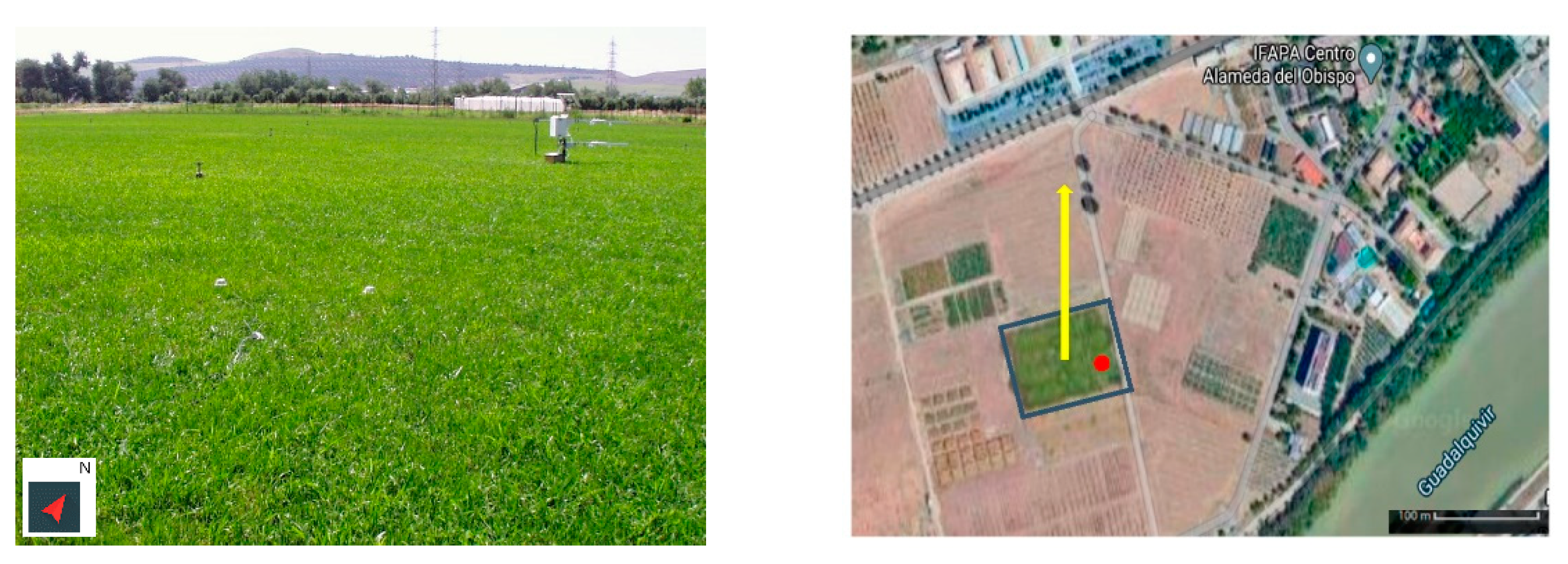
3.1. The Site and Climate

The experiment was carried out from 15 July to 8 September 2009 in the Alameda del Obispo experimental station (37°51′ N, 4°51′ W, 110 m a.s.l) which is located at the IFAPA Agricultural Training and Research Center in Córdoba (Spain). The landscape is flat and agriculture is the main activity. The plot was surrounded by short irrigated crops and bare soils corresponding to other experiments (Figure 1).
In summer, the climate is characterized by the stagnation of the Azores high pressure. Regional advection of sensible heat flux is often severe along the Guadalquivir Valley [44]. The latter understood as that unstable cases are typically observed from dawn to about 14.00 h (local time). Afterwards (i.e., around 2–3 h after noon), positive LE exceeding the available net surface energy is observed until dusk [45,46]. For this case, during the experiment the stability parameter ranged between 0 and 0.22. The prevailing wind direction is west. The weather was typical of the climate which is characterized by clear skies, high temperatures, high evapotranspiration rates and a few short convective rainy events. One short rainy event (about 10 min) was observed during the experiment, and the Table 1 shows the mean maximum and minimum daily values of the maximum and minimum temperatures and the relative humidity of the air, the wind speed, the solar radiation and the evapotranspiration measured with a weighing lysimeter (described next) observed during the experiment.

3.2. Experimental Set Up

A weighing lysimeter was located at the center of a 1.3 ha (110 × 120 m2) rectangular plot of well-watered (sprinkler irrigated) tall-fescue grass (Festuca arundinacea) clipped at about 0.10–0.15 m [45]. The grass was maintained to preserve homogeneity and a fairly constant canopy height. The plot was oriented in the prevailing wind direction and the edge-lysimeter distance was 81 m. The weighing lysimeter consisted of a steel box (3 m × 2 m × 1.5 m deep) measuring half-hourly weight changes with an accuracy of 0.2 kg. Thus, the measurement error is slightly smaller than 50 Wm−2. Soil moisture in and out of the lysimeter were measured at different points using a FDR Diviner probe (Sentek). No trends or spikes were observed along the campaign.
The net radiation was measured half-hourly using a four components net radiometer, CNR1 (Kipp & Zonen). It was deployed adjacent to the lysimeter at 1.5 m height. Half-hourly G was determined using two HFP01 soil heat flux plates (Hukseflux Thermal Sensors, Delft, The Netherlands) and four TCAV soil temperature averaging sensor (Campbell Scientific, Inc., Logan, UT, USA). Below the radiometer, the heat flux plates (placed at 0.08 m depth and separated 1.5 m) were sampled every 10 s, and the mean reading was recorded half hourly. Thermocouples were placed at 0.06 and 0.02 m depth to obtain the half-hourly mean soil temperature above the plates. The soil bulk density and the specific heat capacity was 1.3 g m−3 and 900 J kg−1 K−1, respectively, and the soil heat flux was estimated summing the measured heat flux at 0.08 m and the ground heat storage above the soil heat flux plate [47,48].
A 3-D sonic anemometer and a krypton hygrometer (CSAT3 and KH20, respectively, Campbell Scientific, Inc., Logan, UT, USA) and a fine wire thermocouple (FW05 Campbell Scientific, Inc., Logan, UT, USA) were deployed at 0.9 m and 145 m in the prevailing wind direction. The minimum fetch (North) was 17 m. The distance between the sonic anemometer and the hygrometer measuring paths was 0.11 m. The three wind speed components, sonic and air temperature and humidity fluctuations were measured at 20 Hz and recorded in a memory card using a CR5000 (Campbell Scientific, Inc., Logan, UT, USA) datalogger. The analytical flux-foot print, FFP, model [13] was taken as a guide for instrumentation positioning. The FFP for unstable cases peaked at distances (mean streamwise) between the EC system and the lysimeter. For stable cases, it peaked at distances closer to the lysimeter. Regardless of the stability case, the FFP peaked within the field of view of the outgoing longwave radiation emitted by the surface. Other standard measurements were the half-hourly mean wind speed and direction at 2.0 m (wind monitor RM Young 05103), humidity and temperature of the air at 1.5 m (HMP45C probe, Vaisala, Vantaa, Finland) and precipitation (tipping bucket rain gauge ARG100 deployed at 0.8 m).

3.3. Dataset

After correction of the wind field for flow distortion by transducer shadowing [49], the EC fluxes and turbulent standard deviations were determined using the package TK3 [50], following the protocol taken as a reference in [51]. After excluding the rainy event, periods of maintenance, downwind directions within a sector behind the sonic anemometer (±75°), friction velocities below 0.1 m/s and samples falling within a quality data control classification higher than 8 [50,52,53,54,55], three datasets were formed for different integrated FFP (IFFP) thresholds (taken as a rule of thumb) [13]. Thus, the datasets formed were the following; IFFP ≥ 85% (the maximum value was 92%), 75% < IFFP < 85% and 50% ≤ IFFP ≤ 75%.

3.4. Flux Estimates

The measured sonic temperature, which is close to the virtual temperature [5,15], the temperature of the air and the relative humidity were used to estimate the water vapor pressure, the atmospheric pressure, the density of the air and the specific humidity (q). The latter was used to determine the isobaric specific heat capacity of the air, Cp = (1 + 0.84q) Cpd where Cpd is the isobaric specific heat capacity of dry air (Cpd = 1005 J/(kg K)). The heat of vaporization was calculated as L= −0.0000614342 T3 + 0.00158927 T2 − 2.36418 T + 2500.79 kJ/(kg) where T is the temperature of the air expressed in degrees Celsius [1,5,15]. The von Kármán constant was set to 0.4 [11,28]. The zero-plane displacement and the roughness length for momentum were estimated as a portion of the canopy height, h, d = 0.7h and zo = 0.12h [1]. The ramp dimensions were determined according to [56] as described in [31] (see Appendix A). The sensible heat flux using the SR-P method was determined iterating Equations (1) and (2) because the stability parameter is required as input. Iterations started setting neutral conditions and the criterion for convergence was that the change in friction velocity (i.e., between two consecutive iterations) was smaller than 0.01 m/s [1,22,57]. Once the sensible heat flux was determined, the stability parameter obtained was used as input to determine the first proxy for the latent heat flux, LE0, which was corrected for density fluctuations [50,55]
LE = ( 1 + 1.6 ρ v ρ ) ( LE 0 + L ρ v ρ H C p T )
For the SR-D method, once the sensible heat flux was determined, the latent heat flux obtained using Equation (4) was corrected for density fluctuations. Hence, while the mean wind speed and the trace of the temperature of the air are required as input to estimate the sensible heat flux, in addition, traces of air moisture are required to estimate the latent heat flux.

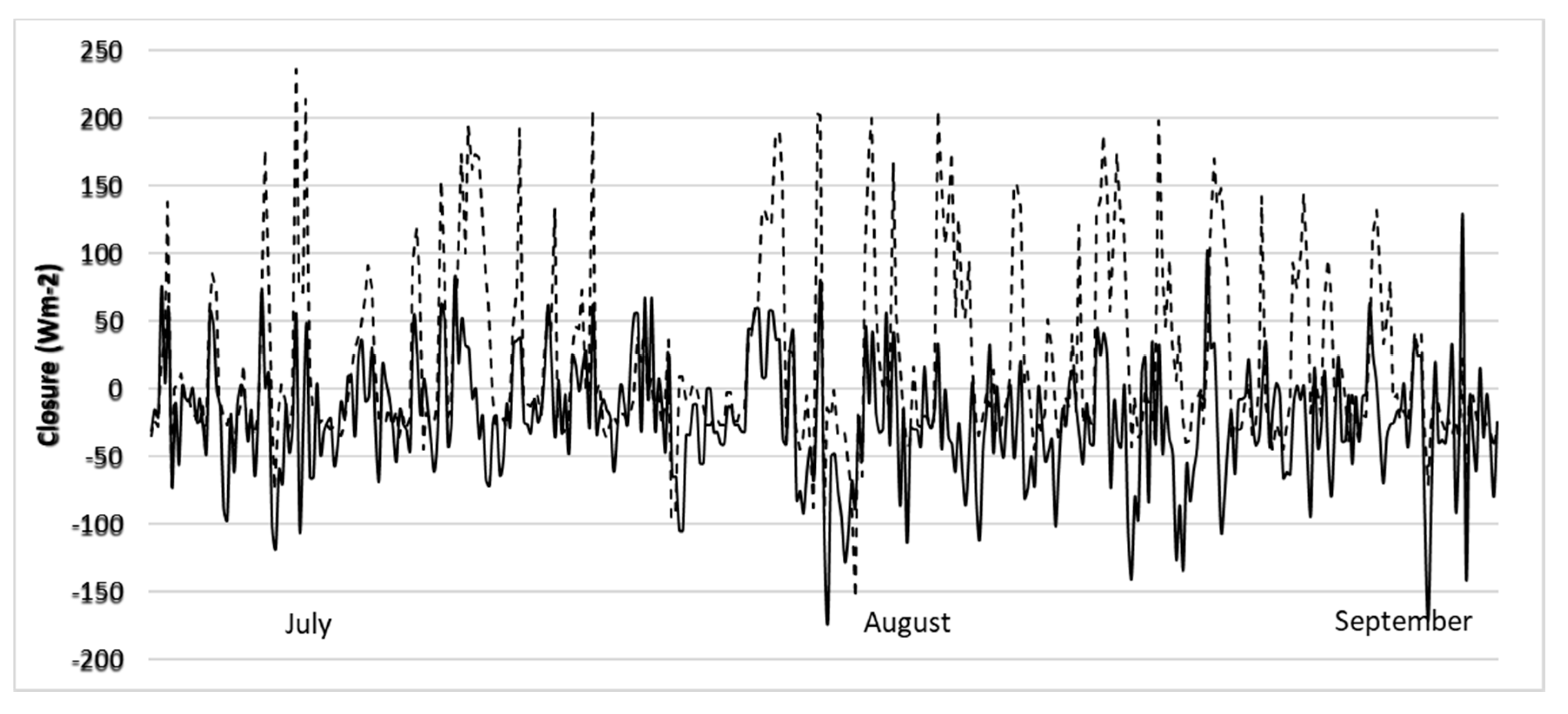
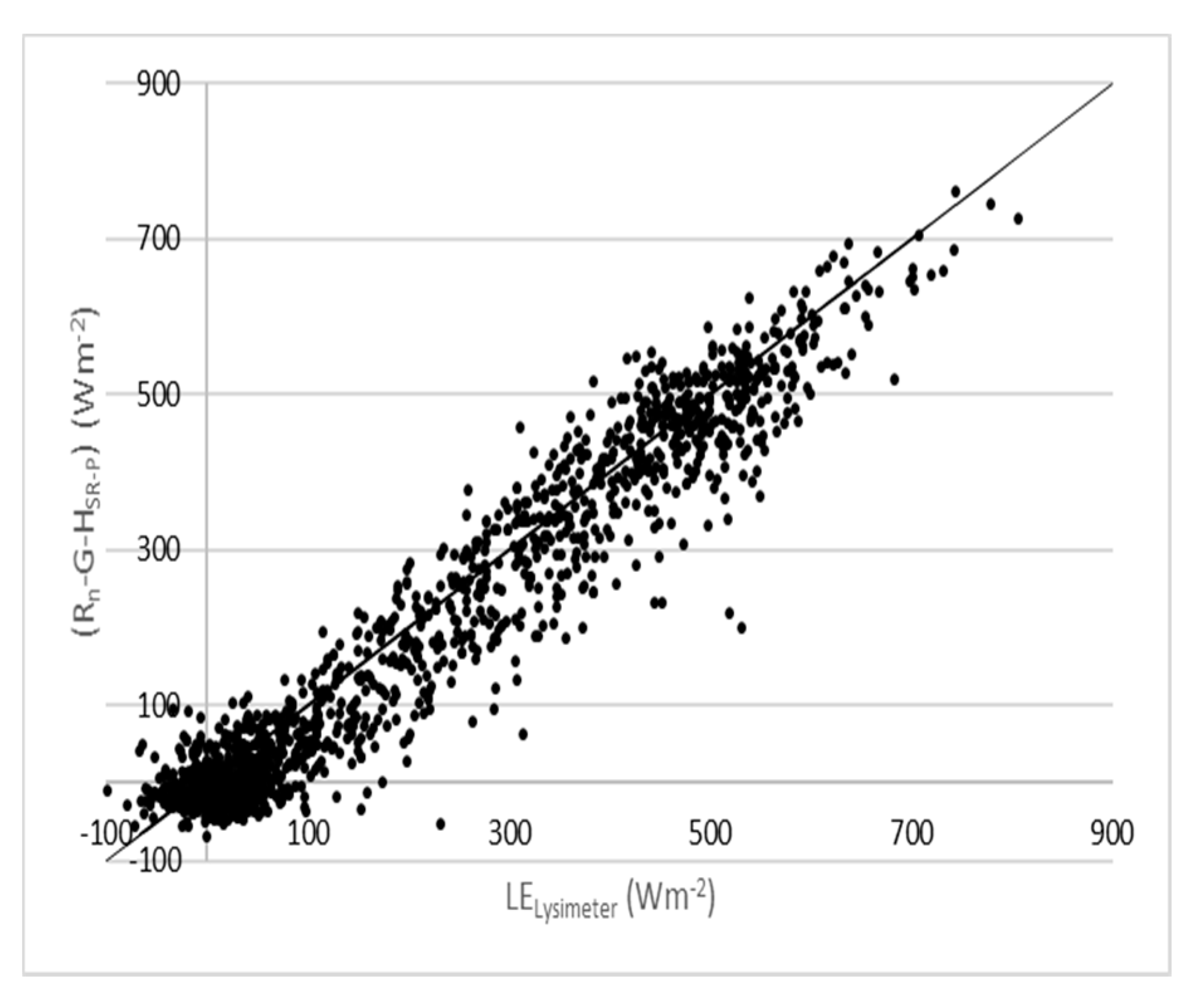
3.5. Procedure for Comparison

The LE determined using the EC method, LEEC, the SR-P method, LESR-P, the SR-D method, LESR-D, and the residual method using different sensible heat flux estimates, (Rn − G − HEC), (Rn − G − HSR-P) and (Rn − G − HSR-D), were compared against the measured using the lysimeter, LELys (reference). The performance was evaluated using linear regression analysis (slope, intercept and coefficient of determination, R2), the root mean square error, RMSE, and the ratio, RD, defined as, RD = y x where variables x and y corresponds to the reference and estimated values, respectively. The coefficient RD is an accumulated ratio used to determine the percentage (p) being over- or underestimated ( p = 100 ( 1 RD ) ) which also gives an integrated evaluation of the bias by averaging out random errors in the half-hourly estimates (i.e., the bias is ( RD 1 ) times the mean reference value determined from the observations).

4. Results

Figure 2 shows the closures (Rn − G − HEC − LELys) and (Rn − G − HEC − LEEC) obtained for all the samples with IFTT ≥ 85% along the experiment. In general, (Rn − G − HEC − LELys) closed the surface energy balance better than (Rn − G − HEC − LEEC). Given that for well-watered crops the net radiation and the latent heat flux dominate the surface energy balance, the Figure 2 suggests that LELys was more reliable than LEEC.
The Table 2 shows the number of samples, N, the slope, a, intercept, b, and the coefficient R2 of the linear regression analysis, the RMSE and the coefficient RD to compare the latent heat flux estimates versus LELys for each dataset and for all the data. Regardless of the IFFP threshold, Table 2 shows that the RD values obtained using LEEC were the worst. In principle, the high coefficients of determination obtained for LEEC are not surprising because the EC method directly measures the turbulence (i.e., EC fluxes are expected highly correlated with the actual eddy fluxes). Therefore, regardless of the underestimation (RD values were smaller than one), LEEC and LELys are expected highly correlated. The Table 2 shows that LESR-P was highly correlated with LELys; in fact, LESR-P did the highest coefficient of determination for the 50% ≤ IFFP ≤ 75% dataset. The slopes of the linear regression analysis obtained using LESR-P were close to the coefficient RD because the intercepts were small and, though LESR-P underestimated the reference, it consistently gave the lowest RMSE. Therefore, LESR-P did the best performance in estimating the latent heat flux in half-hourly basis.
Regardless of the IFFP threshold, Table 2 shows that LESR-D had the lowest correlations, the highest RMSE and the closest RD values to one. This suggested that LESR-D is useful to estimate half-hourly accumulations of latent heat flux.
The disagreement between the LE estimates (LEEC, LESR-P and LESR-D) with respect to LELys increased with the IFFP threshold (Table 2). Comparing the 85% ≤ IFFP and the 50% ≤ IFFP ≤ 75% datasets, the impact in the RD values was of about 30%. It highlights the importance to take measurements within the internal boundary layer. In our case, it reflected the contribution of the drier surroundings to the traces of air moisture.
The impact of insufficient fetch was minimized when the latent heat flux was estimated using the residual method. Though some improvement with respect to LEEC, LESR-P and LESR-D could be expected because the latter require traces of air moisture as input and because (Rn − G) mostly weights to LE for watered surfaces, the close agreement between the estimates and the reference (Table 2) was surprising. The performance for the IFFP < 85% datasets was similar to the IFFP ≥ 85% dataset. In particular, the performance shown in Table 2 for (Rn − G − HEC) and (Rn − G − HSR-P) is similar to the obtained in other experiments over grass with sufficient fetch [58]. Figure 3 compares (Rn − G − HSR-P) against LELys for all the data. It shows that (Rn − G − HSR-P) scattered the full range of LELys and Table 2 shows that the RMSE was similar to the measurement error of LELys (about 50 Wm−2), regardless of the IFFP threshold.
Table 2 shows that (Rn − G − HEC) performed slightly closer to LELys than (Rn − G − HSR-P), but in practice such improvement may not justify the use of the EC method. That is, in terms of cost, the difference between the EC and the SR-P method is significant. In relation to (Rn − G − HSR-D), it consistently gave the closest RD values to one, but the worst R2 and RMSE values. Table 2 shows that (Rn − G − HSR-D) performed similarly to (Rn − G − HEC) and (Rn − G − HSR-P) for the 50% ≤ IFFP ≤ 75% dataset but not as close for the other datasets. The latter was as a consequence that most samples in the 50% ≤ IFFP ≤ 75% dataset were collected near neutral conditions. In any case, (Rn − G − HSR-D) consistently gave RD values close to one; and therefore, it can be recommended to estimate accumulations of latent heat flux.

5. Discussion

Both the flux-gradient relationship and the budget for the turbulent variance of a scalar are principles of physics. Therefore, under the same simplifications (i.e., steady and horizontally homogeneous flow), it must be explained why the SR-P method performed closer to LELys than using the SR-D method. Partly, it can be explained as a consequence that MOST relationships are semi-empirical, being ( ε ) more robust to dissimilarity than σ ( ε ) [59]. The latter implying that the parameter ks may not be expected fairly constant.
It was surprising that LESR-P performed closer to LELys than LEEC and that the best closures of the surface energy balance were obtained using the sensible heat flux determined with the SR-P method. Though it is difficult to explain, for rangeland grass and cotton fields with sufficient fetch, the available net surface energy was slightly better explained using the sum of the sensible heat and the latent heat fluxes determined with the SR-P method than the EC method [57,60]. This explanation is a matter of pending research. Both methods are based on different grounds; the EC method is a simplification of the Navier–Stokes equations, and the SR method is a solution of the mass conservation. Hence, inputs and calculations required are different for each method. In any case, it was shown that the SR-P method has potential for short irrigated crops growing in small plots because it can operate close to the ground, which helps to better match the flux-footprints [14]. Based on MOST, given that similarity relationships tend to become independent of the stability parameter when measurements are taken at low heights, perhaps LESR-D could perform closer to LELys if the instrumentation was deployed at lower heights. Likely, it deserves further research because (according to author’s knowledge) this is the first application of LESR-D.
The combination of the residual method with SR-P sensible heat flux estimates is convenient. The latter not only because the instrumentation required is affordable. Here, the results obtained allow stating that this method can be recommended for irrigated small plots and prior studies have shown excellent performance (i.e., (Rn − G − HSR-P) was close to the LE determined using the EC method and weighing lysimeters) over crops with sufficient fetch [22,23,27,58,60]. It follows that (Rn − G − HSR-P) appears useful for precision agriculture and may allow validating methods or strategies for irrigation. In addition, larger fetches are required to estimate LE when the surface energy balance is forced using the Bowen ratio determined from gradients of temperature and moisture of the air [14,61]. Likely, a two-dimensional sonic anemometer, provided that it allows recording the sonic temperature at high frequency, is the most convenient instrument to estimate HSR-P because it is robust and measures the wind speed with high precision. It allows estimating the ramp dimensions and the friction velocity using different methods [62,63]. When half-hourly latent heat flux accumulations are of interest, (Rn − G − HSR-D) appeared friendly because HSR-D performed as a method exempt of calibration (the errors nearly balanced the accumulated estimates of latent heat flux) and, currently, free-software is available to estimate the ramp dimensions [64]. According to [27,65], likely (Rn − G − HSR-D) is the most affordable and friendly method to estimate latent heat fluxes on a time basis such as daily and weekly. It is worth mentioning that research on the SR-D method to estimate the sensible heat flux operating close to the ground over short canopies is pending.

Author Contributions

F.C.: Conceptualization, Formal analysis, Methodology, Software, Validation, Writing—original draft. P.G.: Conceptualization, Data curation, Validation, Supervision, Writing—original draft. All authors have read and agreed to the published version of the manuscript.

Funding

This research was funded by the National Research Institute of Agriculture and Food Technology (INIA) under the Project RTA2008-00006-CO2-01 and RTI2018-098693-B-C31Ministerio de Economía y Competitividad of Spain.

Institutional Review Board Statement

Not applicable.

Informed Consent Statement

Not applicable.

Data Availability Statement

The datasets analyzed in this study will be available upon request to Pedro Gavilán ([email protected]).

Conflicts of Interest

The authors declare no conflict of interest.

Appendix A. The Surface Renewal Method to Estimate Surface Fluxes

Visual examination of the trace of a scalar measured over a plant canopy or bare soil reveals a ramp-like pattern which has been associated to an organized low-frequency motion (coherent structure). For the trace of the temperature of the air measured under unstable conditions, a ramp-like pattern is shown in Figure A1 that can be idealized as follows [30]. Consider a macroparcel of air (i.e., a parcel which volume per unit area is large enough to contain all the sources) uniformly heated traveling at a given height above the surface. At some instant, it suddenly moves down to the surface where it remains in contact with the sources for a period of time until, by continuity, it is renewed by another parcel sweeping in from above. While the parcel of air remains in contact with the surface heat transfers from the sources to the parcel. Thus, after a nearly steady period (namely quiescent period), the temperature of the air parcel shows a gradual increase (namely warming period) followed by a sudden drop (namely microfront period) to a temperature baseline representing the temperature of a fresh (descending) parcel of air [30,31,56]. The ramp-like pattern is associated to the role of a coherent structure (namely the signature of a coherent structure) where the ejection phase represents an injection of heat into the surface layer.
Figure A1. Time course of the temperature of the air measured at high frequency (dot) for an unstable case. Tb is a baseline temperature representing the mean temperature of a parcel of air that descended to the surface. Quiescent (q), gradual warming (l) and ejection (f) phases are distinguished while the air parcel remains in contact with the surface for a period τ T . Ideally, the mean temperature time course of the air parcel during each phase is assumed linear showing a ramp-like shape in the trace (signature of a coherent structure characterized by a ramp amplitude, A T , and period τ T ). ( A T + T b ) represents the mean temperature of the air parcel when it was renewed.
Atmosphere 12 00322 g0a1
Given that the air parcel is presumed uniformly heated, the ramp amplitude ( A T ) represents its net increase of temperature. Therefore, given that the volume (V) of the air parcel per unit surface (Su) covers all the sources, the amount of heat (QSR) injected to the surface layer above the canopy can be expressed as QSR = (ρCp αZ A T ) where ρ and Cp are the density and the isobaric specific heat capacity of the air, respectively, and (αZ) is the volume of the air parcel per unit area (i.e., V = Su αZ) where Z is the measurement height above the ground and α a correction parameter. A steady coherent structure will inject a regular amount of heat QSR with a frequency 1 / τ T ; and therefore, the sensible heat flux (H) can be estimated as H SR = C p   (   α   Z )   A T / τ T [30]. When the measurements are taken in, the inertial sublayer (αZ) can be estimated as, α Z = [ k π   z   u *   τ T h 1 ( ε ) ] 1 / 2 , where k is the von Kármán constant, z is the measurement heat above the zero-plane displacement, u * is the friction velocity and h ( ε ) is the flux-gradient stability function for heat transfer [22]. Invoking similarity, the latter expression to estimate (αZ) is valid for any scalar. Thus, for latent heat flux, LESR= L (αZ) Aw/τw where L is heat of vaporization and Aw and τw are the amplitude and period in the trace of water vapor density. Clearly, the ramp amplitude in the temperature trace is positive, zero and negative when it is measured under unstable, neutral and stable conditions, respectively. The SR method to estimate surface fluxes requires the analysis of the scalar trace to determine the ramp dimensions; however, a description of these methods is beyond the scope of this paper. A method widely used is based on a ramp model that assumes an instantaneous ejection-sweep phase, that is, a ramp model that neglects the microfront period in Figure A1 [31,56,64]. Accordingly, the mean ramp dimensions can be determined using structure functions of multiple orders ( S n ). For the temperature trace
S n ( r ) = 1 m i = 1 i = m j [ T ( i + j ) T ( i ) ] n
where S denotes structure function, n is the order of the structure function (2nd, 3rd, and 5th), m is the number of data points and j is the sampling lag corresponding to the time lag (r), r = j / f were f is the sampling frequency. The ramp amplitude is obtained by solving for the real roots of the following cubic equation
A T 3 + p A T + q = 0
where p = 10 S 2 ( r ) S 5 ( r ) S 3 ( r ) and q = 10 S 3 ( r ) . Once the ramp amplitude is solved from Equation (A2), the ramp period is determined
τ T = A T 3 r S 3 ( r )
where in Equations (A2) and (A3) r is the time lag that maximizes S 3 ( r ) / r [30], rx. Given that Equations (A2) and (A3) are only valid for time lags r r x and that the determination of rx depends on the sampling frequency (the slope of S 3 ( r ) / r is steep until the global maximum is reached), it is recommended to solve Equations (A2) and (A3) for a time lag slightly higher than rx (i.e., such as the next time lag).

References

  1. Brutsaert, W. Evaporation into the Atmosphere; D. Reidel Publishing Company: Dordrecht, The Netherlands, 1982. [Google Scholar]
  2. Brunet, Y. Turbulent Flow in Plant Canopies: Historical Perspective and Overview. Bound. Layer Meteorol. 2020, 315–364. [Google Scholar] [CrossRef]
  3. Cuxart, J.; Boone, A.A. Evapotranspiration over Land from a Boundary-Layer Meteorology Perspective. Bound. Layer Meteorol. 2020, 427–459. [Google Scholar] [CrossRef]
  4. Shuttleworth, W.J. Putting the vap into evaporation. Hydrol. Earth Syst. Sci. 2007, 11, 210–244. [Google Scholar] [CrossRef] [Green Version]
  5. Foken, T. Micrometeorology; Springer: Berlin/Heidelberg, Germany, 2008. [Google Scholar]
  6. Twine, T.E.; Kustas, W.P.; Norman, J.M.; Cook, D.R.; Houser, P.R.; Meyers, T.P.; Prueger, J.H.; Starks, P.J.; Wesely, M.L. Correcting eddy-covariance flux underestimates over a grassland. Agric. Forest Meteorol. 2000, 103, 279–300. [Google Scholar] [CrossRef] [Green Version]
  7. Pereira, L.S.; Allen, R.G.; Smith, M.; Raes, D. Crop evapotranspiration estimation with FAO56: Past and future. Agric. Water Manag. 2015, 147, 4–20. [Google Scholar] [CrossRef]
  8. de Bruin, H.A.R.; Trigo, I.F.; Bosveld, F.C.; Meirink, J.F. A thermodynamically based model for actual evapotranspiration of an extensive grass field close to FAO Reference, suitable for remote sensing application. J. Hydrometeorol. 2016, 17, 1373–1382. [Google Scholar] [CrossRef]
  9. Castellví, F.; Medina, E.; Cavero, J. Surface eddy fluxes and friction velocity estimates taking measurements at the canopy top. Agric. Water Manag. 2020, 241, 106358. [Google Scholar] [CrossRef]
  10. Castellví, F.; Suvočarev, K.; Reba, M.; Runkle, B. A new free-convection form to estimate sensible heat and latent heat fluxes for unstable cases. J. Hydrol. 2020, 586, 124917. [Google Scholar] [CrossRef]
  11. Stull, R.B. An Introduction to Boundary Layer Meteorology; Atmospheric and Oceanographic Sciences Library; Springer: Cham, Switzerland, 1988. [Google Scholar]
  12. Graefe, J. Roughness layer corrections with emphasis on SVAT model applications. Agric. For. Meteorol. 2004, 124, 237–251. [Google Scholar] [CrossRef]
  13. Horst, T.W.; Weill, J.C. How far is far enough?: The fetch requirements for micrometeorological measurement of surface fluxes. J. Atmos. Ocean. Technol. 1994, 11, 1018–1025. [Google Scholar] [CrossRef] [Green Version]
  14. Castellví, F. Fetch requirements using surface renewal analysis for estimating scalar surface fluxes from measurements in the inertial sublayer. Agric. Forest Meteorol. 2012, 152, 233–239. [Google Scholar] [CrossRef]
  15. Burba, G.; Anderson, D. Introduction to the Eddy Covariance Method: General Guidelines and Conventional Workflow; LI-COR Biosciences: Lincoln, NE, USA, 2007; 141p, ISBN 1951D438-A0374350-AA92950EFF6457. [Google Scholar] [CrossRef]
  16. Aubinet, M.; Vesala, T.; Papale, D. Eddy Covariance: A Practical Guide to Measurement and Data Analysis; Springer: Berlin/Heidelberg, Germany, 2012. [Google Scholar]
  17. Noltz, R.; Krammerer, G.; Cepuder, P. Interpretation of lysimeter weighing data affected by wind. J. Plant Nutr. Soil Sci. 2013, 176, 200–208. [Google Scholar] [CrossRef]
  18. Silva, J.C.; Silva, T.J.A.; Bonfim-Silva, E.M.; Duarte, T.F.; Pacheco, A.B. Construction and assessment of a hydraulic weighing lysimeter. Afr. J. Agric. Res. 2016, 11, 951–960. [Google Scholar]
  19. Haymann, N.; Lukyanova, V.; Tanny, J. Effects of variable fetch and footprint on surface renewal measurements of sensible and latent heat fluxes in cotton. Agric. For. Meteorol. 2019, 124, 237–251. [Google Scholar] [CrossRef]
  20. Jegede, O.O.; Foken, T. A study of the internal boundary layer due to a roughness change in neutral conditions observed during the LINEX field campaigns. Theor. Appl. Climatol. 1999, 62, 31–41. [Google Scholar] [CrossRef]
  21. Levy, P.; Drewera, J.; Jammeta, M.; Leeson, S.; Friborgb, T.; Skibaa, U.; Van Oijena, M. Inference of spatial heterogeneity in surface fluxes from eddy covariance data: A case study from a subarctic mire ecosystem. Agric. For. Meteorol. 2020, 280, 107783. [Google Scholar] [CrossRef]
  22. Castellví, F. Combining surface renewal analysis and similarity theory: A new approach for estimating sensible heat flux. Water Resour. Res. 2004, 40, W05201. [Google Scholar] [CrossRef] [Green Version]
  23. Castellvi, F.; Snyder, R.L. Combining the dissipation method and surface renewal analysis to estimate scalar fluxes from the time traces over rangeland grass near Ione (California). Hydrol. Process. 2009, 23, 842–857. [Google Scholar] [CrossRef]
  24. Kustas, W.P.; Norman, J.M. Evaluation of soil and vegetation heat flux predictions using a simple two-source model with radiometric temperatures for partial canopy cover. Agric. For. Meteorol. 1999, 94, 13–29. [Google Scholar] [CrossRef]
  25. Jiang, L.; Islam, S.; Carlson, T.R. Uncertainties in latent heat flux measurement and estimation: Implications for using a simplified approach with remote sensing data. Can. J. Rem. Sens. 2004, 30, 769–787. [Google Scholar] [CrossRef]
  26. Bisht, G.; Venturini, V.; Islam, S.; Jiang, L. Estimation of the net radiation using MODIS (Moderate Resolution Imaging Spectroradiometer) data for clear sky days. Remote Sens. Environ. 2005, 97, 52–67. [Google Scholar] [CrossRef]
  27. Hu, Y.; Buttar, N.A.; Tanny, J.; Snyder, R.L.; Savage, M.J.; Lakhiar, I.A. Surface renewal application for estimating evapotranspiration: A review. Adv. Meteorol. 2018, 1690714. [Google Scholar] [CrossRef] [Green Version]
  28. Högström, U. Review of some basic characteristics of the atmospheric surface layer. Bound. Layer Meteorol. 1996, 78, 215–246. [Google Scholar] [CrossRef]
  29. Higbie, R. The rate of absorption of a pure gas into a still liquid during short periods of exposure. Trans. AIChE 1935, 31, 365–388. [Google Scholar]
  30. Paw, U.K.T.; Qiu, J.; Su, H.B.; Watanabe, T.; Brunet, Y. Surface renewal analysis: A new method to obtain scalar fluxes without velocity data. Agric. Forest Meteorol. 1995, 74, 119–137. [Google Scholar]
  31. Chen, W.; Novak, M.D.; Black, T.A.; Lee, X. Coherent eddies and temperature structure functions for three contrasting surfaces. Part I: Ramp model with finite micro-front time. Bound. Layer Meteorol. 1997, 84, 99–123. [Google Scholar] [CrossRef]
  32. Castellví, F. A method for estimating the sensible heat flux in the inertial sub-layer from high-frequency air temperature and averaged gradient measurements. Agric. Forest Meteorol. 2013, 180, 68–75. [Google Scholar] [CrossRef]
  33. Dyer, A.J. A review of flux-profile relationships. Bound. Layer Meteorol. 1974, 363–372. [Google Scholar] [CrossRef]
  34. Panofsky, H.; Dutton, J. Atmospheric Turbulence: Models and Methods for Engineering Applications; John Wiley: New York, NY, USA, 1984. [Google Scholar]
  35. Pahlow, M.; Parlange, M.B.; Port’e-Agel, F. On Monin-Obukhov similarity in the stable atmospheric boundary layer. Bound. Layer Meteorol. 2001, 99, 225–248. [Google Scholar] [CrossRef] [Green Version]
  36. Hartogensis, O.K.; de Bruin, H.A.R. Monin-Obukhov similarity function of the structure parameter of temperature and turbulent kinetic energy dissipation rate in the stable boundary layer. Bound. Layer Meteorol. 2005, 116, 253–276. [Google Scholar] [CrossRef]
  37. Champagne, F.H.; Friehe, C.A.; Larue, J.C. Flux measurements, flux estimation techniques, and Fine-Scale turbulence measurements in the unstable surface layer over land. J. Atmos. Sci. 1977, 34, 515–530. [Google Scholar] [CrossRef] [Green Version]
  38. Antonia, R.A.; Chambers, A.J.; Friehe, C.A.; Van Atta, C.W. Temperature ramps in the atmospheric surface layer. J. Atmos. Sci. 1979, 36, 99–108. [Google Scholar] [CrossRef] [Green Version]
  39. Bradley, E.R.; Antonia, R.A.; Chambers, A.J. Temperature structure in the atmospheric surface layer. Bound. Layer Meteorol. 1981, 20, 275–292. [Google Scholar] [CrossRef]
  40. Kader, B.A. Determination of turbulent momentum and heat fluxes by spectral methods. Bound. Layer Meteorol. 1992, 61, 323–347. [Google Scholar] [CrossRef]
  41. Kiely, G.; Albertson, J.D.; Parlange, M.B.; Eichinger, W.E. Convective scaling of the average dissipation rate of tempearture variance in the atmospheric surface layer. Bound. Layer Meteorol. 1996, 77, 267–284. [Google Scholar] [CrossRef] [Green Version]
  42. Hsieh, C.I.; Katul, G.G.; Schieldge, J.; Sigmon, J.; Knoer, K.R. Estimation of momentum and heat fluxes using dissipation and flux-variance methods in the unstable surface layer. Water Resour. Res. 1996, 32, 2453–2462. [Google Scholar] [CrossRef]
  43. Hsieh, C.I.; Katul, G.G. Dissipation methods, Taylor’s hypothesis, and stability correction functions in the atmospheric surface layer. J. Geophys. Res. 1997, 102, 16391–16405. [Google Scholar] [CrossRef] [Green Version]
  44. Hernández-Ceballos, M.A.; Adame, J.A.; Bolívar, J.P.; De la Morena, B.A. A mesoscale simulation of coastal circulation in the Guadalquivir valley (southwestern Iberian Peninsula) using the WRF-ARW model. Atmos. Res. 2013, 24, 1–20. [Google Scholar] [CrossRef]
  45. Berengena, J.; Gavilán, P. Reference evapotranspiration estimation in a highly advective semiarid environment. J. Irrig. Drain. Eng. 2005, 131, 147–163. [Google Scholar] [CrossRef]
  46. Gavilán, P.; Berengena, J. Accuracy of the Bowen ratio-energy balance method for measuring latent heat flux in a semiarid advective environment. Irrig. Sci. 2007, 25, 127–140. [Google Scholar] [CrossRef]
  47. Fuchs, M.; Tanner, C.B. Evaporation from a drying soil. J. Appl. Meteorol. 1967, 6, 852–857. [Google Scholar] [CrossRef] [Green Version]
  48. Sauer, T.J.; Horton, R. Soil heat flux. In Micrometeorology in Agricultural Systems ASA Monograph; Hatfield, J.L., Baker, J.M., Eds.; American Society of Agronomy: Madison, WI, USA, 2005; Chapter 7; Volume 47, pp. 131–154. [Google Scholar] [CrossRef]
  49. Horst, T.W.; Semmer, S.R.; Maclean, G. Correction of a non-orthogonal, three-component sonic anemometer for flow distortion by transducer shadowing. Bound. Layer Meteorol. 2015, 155, 371–395. [Google Scholar] [CrossRef] [Green Version]
  50. Mauder, M.; Foken, T. Documentation and Instruction Manual of the Eddy Covariance Software Package TK3 46; Abt. Mikrometeorologie, Arbeitsergebnisse; Universität Bayreuth: Bayreuth, Germany, 2011; p. 56. [Google Scholar]
  51. Mauder, M.; Oncley, S.P.; Vogt, R.; Weidinger, T.; Ribeiro, L.; Bernhofer, C.; Foken, T.; Kosiek, W.; de Bruin, H.A.R.; Liu, H. The energy balance experiment EBEX-2000. Part II: Intercomparison of eddy-covariance sensors and post-field data processing methods. Bound. Layer Meteorol. 2007, 123, 29–54. [Google Scholar] [CrossRef]
  52. Vickers, D.; Mahrt, L. The cospectral gap and turbulent flux calculations. J. Atmos. Ocenanic Technol. 2002, 20, 660–672. [Google Scholar] [CrossRef]
  53. Van de Wiel, B.J.H.; Moene, A.F.; Hartogensis, O.K.; de Bruin, H.A.R.; Holtslag, A.A.M. Intermittent turbulence in the stable boundary layer over land. Part III: A classification for observations during CASES-99. J. Atmos. Sci. 2003, 60, 2509–2522. [Google Scholar] [CrossRef]
  54. Steeneveld, G.J.; VandeWiel, B.J.H.; Holtslag, A.A.M. Modelling the evolution of the atmospheric boundary layer coupled to the land surface for a three day period in CASES-99. J. Atmos. Sci. 2006, 63, 920–935. [Google Scholar] [CrossRef]
  55. Burba, G. Eddy Covariance Method for Scientific, Industrial, Agricultural and Regulatory Applications; LiCor Biosciences: Lincoln, NE, USA, 2013. [Google Scholar]
  56. Van Atta, C.W. Effect of coherent structures on structure functions of temperature in the atmospheric boundary layer. Archit. Mech. 1977, 29, 161–171. [Google Scholar]
  57. Suvočarev, K.; Castellví, F.; Reba, M.L.; Runkle, B.R.K. Surface renewal measurements of H, λE and CO2 fluxes over two different agricultural systems. Agric. Forest Meteorol. 2019. [Google Scholar] [CrossRef]
  58. Castellví, F.; Snyder, R.L. A comparison between latent heat fluxes over grass using a weighing lysimeter and surface renewal analysis. J. Hydrol. 2010, 381, 213–220. [Google Scholar] [CrossRef]
  59. Katul, G.G.; Hsieh, C.I. A Note on the Flux-Variance Similarity Relationships for Heat and Water Vapour in the Unstable Atmospheric Surface Layer. Bound. Layer Meteorol. 1999, 90, 327–338. [Google Scholar] [CrossRef]
  60. Castellví, F.; Snyder, R.L.; Baldocchi, D.D. Surface energy-balance closure over rangeland grass using the eddy covariance method and surface renewal analysis. Agric. Forest Meteorol. 2008, 148, 1147–1160. [Google Scholar] [CrossRef]
  61. Horst, T.W. The footprint for estimation of atmosphere–surface exchange fluxes by profile techniques. Bound. Layer Meteorol. 1999, 90, 171–188. [Google Scholar] [CrossRef]
  62. Castellví, F. An advanced method based on surface renewal theory to estimate the friction velocity and the surface heat flux. Water Resour. Res. 2018, 54, 10134–10154. [Google Scholar] [CrossRef]
  63. Castellví, F.; Suvočarev, K.; Reba, M.; Runkle, B. Friction velocity estimates using the trace of a scalar and the mean wind speed. Bound. Layer Meteorol. 2020, 176, 105–123. [Google Scholar] [CrossRef]
  64. Kelley, J.; Higgins, C. Computational efficiency for the surface renewal method. Atmos. Meas. Tech. 2018, 11, 2151–2158. [Google Scholar] [CrossRef] [Green Version]
  65. Drexler, J.Z.; Snyder, R.L.; Spano, D.; Paw, U.K.T. A review of models and micrometeorological methods used to estimate wetland evapotranspiration. Hydrol. Process. 2004, 18, 2071–2101. [Google Scholar] [CrossRef]
Figure 1. Meteorological station nearby the lysimeter (left) and aerial view (Google Maps, 6 February 2021) of the experimental plot (blue rectangle) in the IFAPA center Alameda del Obispo nearby the Guadalquivir river (right). The lysimeter and the tower were positioned as indicate the yellow arrow (pointing North) and the red area, respectively.
Atmosphere 12 00322 g001
Figure 2. (Rn − G − HEC − LELys), solid line, and (Rn − G − HEC − LEEC), dashed line, values for samples with IFTT ≥ 85%. The x-axis shows chronological order.
Atmosphere 12 00322 g002
Figure 3. (Rn − G − HSR-P) against the reference for all the data. The 1:1 ratio line (thin solid) is shown.
Atmosphere 12 00322 g003
Table 1. Climatology observed during the experiment.
Daily Mean:TxTnHRxHRnURsET
(°C)(°C)(%)(%)(m/s)(MJ/Day)(mm/Day)
Maximum39.923.285.634.63.332.39.2
Minimum31.114.245.58.10.917.24.3
Average35.819.066.515.91.927.87.2
Tx and Tn, maximum and minimum temperature of the air, respectively; HRx and HRn, maximum and minimum relative humidity of the air, respectively; U, wind speed; Rs, solar radiation; ET, evapotranspiration.
Table 2. Comparison of the latent heat flux estimates versus the reference (lysimeter).
Dataset: N = 41785% ≤ IFFP
abR2RMSERD
Method:(Wm−2)(Wm−2)
LEEC0.7130.96730.73
LESR-P0.8560.91600.9
LESR-D0.9250.77931.07
Rn − G − HEC1−220.95480.86
Rn − G − HSR-P0.96−230.95520.81
Rn − G − HSR-D0.96150.88701.07
N = 74975% < IFFP < 85%
LEEC0.6950.96980.71
LESR-P0.8620.91730.87
LESR-D0.87210.711240.96
Rn − G − HEC1−190.95540.9
Rn − G − HSR-P0.97−180.94570.88
Rn − G − HSR-D0.99190.86861.08
N = 44550% ≤ IFFP ≤ 75%
LEEC0.5250.831330.55
LESR-P0.5530.91250.56
LESR-D0.690.711360.64
Rn − G − HEC1.05−50.94511.02
Rn − G − HSR-P0.99−70.94490.95
Rn − G − HSR-D130.92551.01
N = 161150% ≤ IFFP (all data)
LEEC0.6530.911040.67
LESR-P0.7910.86880.79
LESR-D0.8180.691200.89
Rn − G − HEC1.01−150.95520.93
Rn − G − HSR-P0.98−160.94540.89
Rn − G − HSR-D0.99140.88761.06
N, number of samples; IFFP, integrated flux-foot print; a, b and R2, slope, intercept and determination coefficient of the linear regression analysis, respectively; RMSE, root mean square error; RD, accumulated latent heat flux estimates over the reference.
Publisher’s Note: MDPI stays neutral with regard to jurisdictional claims in published maps and institutional affiliations.

