Abstract
The interplanetary medium variability has been extensively studied by means of different approaches showing the existence of a wide variety of dynamical features, such as self-similarity, self-organization, turbulence and intermittency, and so on. Recently, by means of Parker solar probe measurements, it has been found that solar wind magnetic field fluctuations in the inertial range show a clear transition near 0.4 AU, both in terms of spectral features and multifractal properties. This breakdown of the scaling features has been interpreted as the evidence of a dynamical phase transition. Here, by using the Klimontovich S-theorem, we investigate how the process of self-organization is under way through the inner heliosphere, going deeper into the characterization of this dynamical phase transition by measuring the evolution of entropic-based measures through the inner heliosphere.
1. Introduction
During the past fifty years, several properties of the solar wind magnetic field fluctuations have been investigated, by means of both spacecraft data and numerical simulations [1,2,3,4]. From earlier space missions to more recent ones, a lot of attention has been paid to investigate the statistical properties of the different dynamical regimes in terms of statistics of increments [5], scaling law behavior [6], turbulence and intermittency [7], energy transfer rate [8], cascade vs. stochastic processes [9], and so on [10]. While earlier space missions (e.g., Helios, Ulysses, ACE, Wind) allowed one to characterize the physical properties at MHD scales [11,12,13], the more recent ones (e.g., Cluster, MMS) can allow us to deeply investigate from sub-ion down to electron scales [14,15]. Moreover, the recently launched Parker solar probe (PSP) can really be helpful to investigate how the dynamical properties of the solar wind evolve through the heliosphere, allowing us for the first time to reach the closest distances (∼0.17 AU) to the Sun [16,17]. Despite its recent launch (i.e., August 2018), it has still completed 6 orbits around the Sun and it has allowed us to explore a much different picture of the solar wind near the Sun with respect to that observed near the Earth, as for example, the emergence of flips in the direction of the magnetic field, named switchbacks [18,19], lasting anywhere from a few seconds to several minutes, or remnants of structures have been detected near and far from the Sun, being hurled into space and changing the topology of the solar wind plasma and magnetic field [20]. Furthermore, thanks to its journey around the Sun, PSP allowed to characterize the behavior of scaling regimes at different Heliocentric distances [21], also showing for the first time the occurrence of a dynamical transition near 0.4 AU from a monofractal to a multifractal underlying structure of the magnetic field fluctuations across the inertial range of scales [22]. This transition is necessarily related to something that breaks the phase-coherency of inertial range fluctuations, leading to the breakdown of the scaling properties of the energy transfer rate. Indeed, in the usual formalism of turbulence, the q-th order structure function of the field , defined in terms of increments at a scale ℓ, follows a power-law behavior as
being D the “effective” dimension of the system, depending on the degree of freedom of the system itself [23,24]. However, both fluids and plasmas are characterized by anomalous scaling features, being the fluctuations of the energy transfer rate depending on ℓ, i.e., , usually interpreted as the evidence of intermittency [25,26,27], such that
Since for monofractal fields then closer to the Sun there could be some physical mechanisms, as a strong Alfvénicity and/or a reduced compressibility [21], that are able to suppress the scaling behavior of the energy transfer rate [22], thus making and then ; conversely, as larger heliocentric distances (e.g., greater than 0.4 AU) are reached the solar wind expansion can lead to a different scaling, leaving far from the Sun, thus providing , and suggesting an effective dimension , as based on solar wind observations [2]. These findings can be also described in a complex system framework, as the emergence of a dynamical phase transition in dependence of the heliocentric distance r, then the scaling exponents can be written as
being a smooth nonlinear convex function of q [22].
The above findings seem to suggest that more speculations can be investigated by means of complex system-based approaches [28], allowing us a different view of the topological properties of the solar wind magnetic field fluctuations. Indeed, the solar wind, instead of being “only” considered a natural laboratory for plasma physics [2], is an example of multiscale dynamical system, evolving through the heliosphere, with completely different properties across the different dynamical regimes. As an example, the inertial range can be interpreted as an unstable fixed point of the MHD equations [29], being characterized by a low-dimensional attractor that can be also easily described via a discrete dynamical system [30]; conversely, a more ergodic-like behavior is found for the sub-ion/dissipative regime in terms of its phase-space topology, being characterized by fractal dimensions mostly approaching the full dimension of the system [29]. Moreover, both regimes are also characterized by different fractal topological structures, the inertial range being more intermittent than the dissipative one, reflecting its multifractal nature with respect to the monofractal behavior observed at dissipative scales [29]. These seem to suggest to further explore the solar wind nature by means of dynamical systems approaches and complex system-based tools [31].
In the framework of open systems, Klimontovich [32] introduced a theorem, namedKlimontovich self-organization theorem (S-theorem), to quantify the degree of order in open nonequilibrium stationary states. Indeed, due to the emergence of coherence, self-organization and correlations in such nonequilibrium systems, we may assist to a reduction of the physical chaos (uncorrelated motion of particles). The Klimontovich S-theorem establishes a criterion to measure the relative degree of self-organization in open systems.
Here, using the solar wind magnetic field data collected during the first and second encounter of Parker solar probe to the Sun, we investigate how the properties of fluctuations evolve with the heliocentric distance by applying the Klimontovich S-theorem, allowing us a more proper characterization of self-organization through the inner heliosphere. In detail, we investigate the occurrence of a dynamical phase transition by means of the degree of self-organization and attempt to identify the physical quantity responsible for the emergence of such a dynamical transition.
2. The Klimontovich S-Theorem
In the framework of open nonequilibrium dynamical systems near a stationary state, two of the most important questions are:
- how to compare states characterized by different values of a control parameter and
- how to compare their relative degree of chaos or provide a measure of the relative degree of self-organization.
Indeed, when the value of the control parameter changes, the system can recede from the equilibrium/stationary state approaching a different state. In such a process, one can assist the emergence of a self-organization phenomenon in which part of the energy is spent in correlations between the constituents of the system. As a consequence of the emergence of self-organization, the system can undergo to a transition towards another stationary state characterized by a different entropy value, i.e., we can assist to a variation of the amount of entropy S. Because in the framework of statistical mechanics the equilibrium state refers to the stationary, space-invariant state characterized by the maximum value of entropy according to the fixed external constraints, a departure from this state should be associated with a decrease in the amount of entropy, i.e., we are in the presence of a reduction of the entropy of the new state in respect to the equilibrium state value ,
The observed entropy variation is, generally, a consequence of the emergence of correlations which have the effect of reducing the effective number of degrees of freedom of the system.
According to Klimontovich [32], it is possible to derive a method to compare the degree of self-organization between two stationary states by means of an entropic functional, directly approaching to the problem using Boltzmann’s H-theorem.
Let be the probability distribution of the equilibrium state and let be the one for a nonequilibrium state (which, by definition, depends upon time) in the case of an isolated/closed system. Then, we know that if when , according to the H-theorem, the functional H must satisfy:
being the support over which the distributions are defined. Mathematically speaking, the functional H is the Kullback–Leibler divergence, i.e., the distance in probability between and which is a measure of the error in describing the dynamical process X by means of when the real distribution is . In other words, the above quantity provides a measure of the distance from the equilibrium state in terms of a variation of entropy.
The above considerations were extended by Ref. [32] and Klimontovich [33] to compare the degree of self-organization between different stationary states depending on a control parameter in the case of open nonequilibrium systems. This is formulated in what is known as Klimontovich S-theorem.
Because the change of a control parameter from a certain value to a different one , i.e., in the case of open systems does not ensure that energy is conserved, the direct comparison between the entropy values of two states characterized by a different values of the control parameter to estimate the degree of self-organization is not feasible. Klimontovich S-theorem [32,33] solves this problem by constraining the distributions to have the same energy (information content) in order to be compared. In order to do this, we introduce the effective Hamiltonian , defined by
where is the distribution function associated with the state with control parameter , which is taken as the reference state. Then, if is the distribution function associate with the new state characterized by a control parameter , the S-theorem requires to renormalize the reference state distribution function, so that , i.e.
where is the renormalized reference state , which is defined as
where is an effective temperature that is obtained by solving the Equation (7). This effective temperature is expected to be if the reference state is the one of maximum chaos (i.e., the more entropic one), otherwise . In this framework, the effective temperature is the quantity appointed to estimate the degree of self-organization, providing an estimate of the fraction of energy spent in correlations, i.e., is a measure of the energy/heat to add to the reference state to change it into the more organized state .
Now, in this framework, the function in Equation (5) is replaced by the relative entropy given by
We emphasize that the relative entropy given above can be regarded as the relative entropy in terms of difference between two-states entropies if
In other words, the entropy of the equilibrium state is given by the mean effective energy computed over the nonequilibrium stationary distribution [34]. Thus, we can argue that the Equation (9) becomes
It is important to remark that if the result of the Equation (7) returns a value , then it means that the state of maximum chaos is not the state “0”, but the state “1”, so that for a correct evaluation of the entropy, variation is necessary to exchange the two states.
3. Data Description and Methods
3.1. Data
In this work, we use magnetic field measurements collected by the FIELDS instrument onboard the Parker solar probe (PSP) at 4 sample-per-cycle cadence [16,35]. In particular, we focus on two already investigated time intervals [21,22], when the PSP approached the inner heliosphere. These two time intervals refer to the first and the second encounters, from 15 October 2018 to 14 December 2018 (first encounter), and from 16 March 2019 to 10 April 2019 (second encounter), respectively. During these time intervals, PSP explored the inner heliosphere in the range between 0.17 AU and 0.66 AU near the heliospheric equator. A detailed discussion of the physical conditions of the two selected time intervals can be found in Alberti et al. [22] and Chen et al. [21].
Data are released in the heliocentric radial-tangential-normal (RTN) reference system and freely retrieved from the Space Physics Data Facility (SPDF) Coordinated Data Analysis Web (CDAWeb) interface at https://cdaweb.gsfc.nasa.gov/index.html/ (accessed on 8 February 2021). Here, we consider the magnetic field normal component () and intensity resampled at a resolution of 1 s. This choice is related to the fact that the normal component is typically the best one to be analyzed in the framework of turbulence and self-organization, being less affected by the large scale interplanetary magnetic field (IMF) structure (i.e., the Parker spiral structure) and velocity field changes [36].
Figure 1 shows the behavior of the magnetic field intensity, , and its normal component, , for the two selected time intervals separately. According to the Parker theory [37], the magnetic field intensity depends on the distance from the Sun on as shown in Figure 2, where we report the behavior of the magnetic field intensity (averaged using data from both the encounters) as a function of the radial distance R.
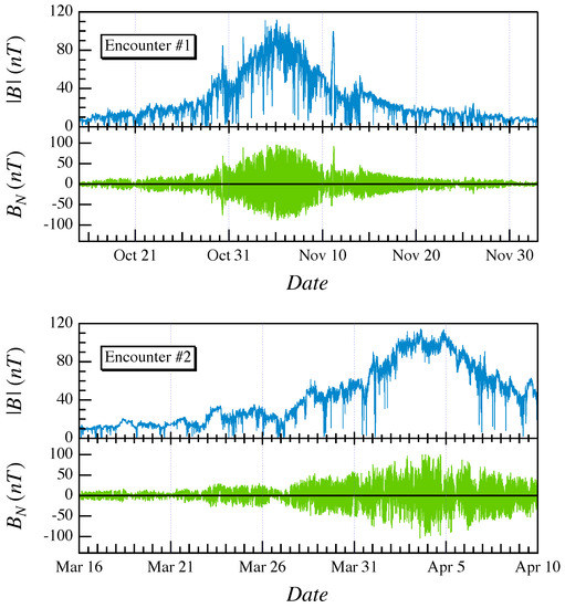
Figure 1.
The magnetic field intensity () and the normal component () for the two selected time intervals relative to the first (upper plots) and second (lower plots), respectively.
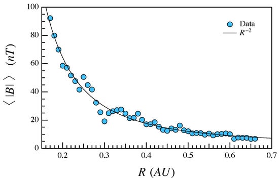
Figure 2.
The average magnetic field intensity () as a function of the radial distance, R. The solid line is a power-law fit according to expected scaling with the distance, i.e., .
Since we will focus our analysis on the inertial range dynamics, the magnetic field normal component has been filtered to remove the long time trend using a high-pass filter with a frequency cut-off Hz. Figure 3 shows the power spectral density (PSD) of the original time series for the first encounter together with those corresponding to the filtered time series below and above the frequency cut-off , while Figure 4 shows the filtered time series, , for both time intervals.
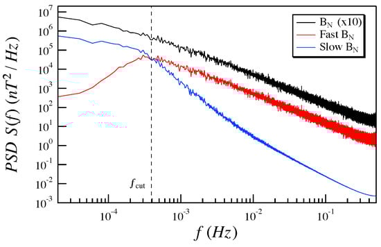
Figure 3.
The power spectral density (PSD) of the original time series of the normal component together with those corresponding to the filtered time series below and above the frequency cut-off . The PSD of the normal component has been scaled by a factor 10 for visual purposes.
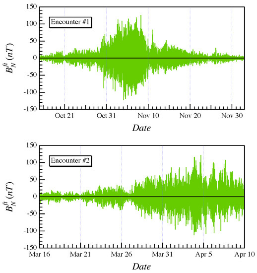
Figure 4.
The filtered time series for both the first and the second encounter.
3.2. Methods
As discussed in Section 2, the most important quantity to be evaluated using the Klimontovich S-theorem is the effective temperature , being the quantity necessary to evaluate the entropy reduction/variation . This can be done by numerically solving the integral equation (7), which can be recast in a root finding problem for the function defined by
where and are, respectively, the left-hand side and the right-hand side of Equation (7), i.e.,
and
Thus, the effective temperature is that for which .
In our analysis, Equation (13) is solved using the Newton–Raphson method (also known as tangent method) with a tolerance value .
The effective temperature provides a quantitative measure of the relative order between two selected states: if , the state “0” is more disordered than the state “1”; otherwise, the state “1” is more disordered than the state “0”. This means that, when comparing more than two signals, we firstly need to identify the reference state, i.e., the state of maximum physical chaos. To this purpose, it is useful to introduce a matrix , which we call disorder matrix, whose elements are defined by following the meaning of effective temperature:
where is the effective temperature found by imposing the renormalization to distribution and by fixing the distribution. In this framework, the more disordered state i can be defined as the one satisfying the condition
Another important issue in solving Equation (7) is the correct evaluation of the distribution functions . In this work, we use a uniform-binning method to evaluate distributions. Furthermore, in order to compare the distributions for different values of the selected control parameter (here the radial distance R), we must define a common grid over which and are computed. The grid (or support) is a uni-dimensional vector whose sup and inf correspond to the maximum and minimum value of the concatenated signal amplitudes, respectively. In other words, let and be the signals corresponding to control parameters and , respectively, then the concatenated signal is given by (for all i and j, if more than two signals have to be compared). Thus, if and , then .
Since the estimation of is done by solving an integral equation, and since the integration step is the distance between two near grid-points, clearly the precision of the algorithm is a function of the number of bins chosen to estimate and . In detail, the numerical approximation is better the smaller the integration step is, and thus, the number of bins has to be sufficiently large. On the other hand, if the number of bins is too large, each bin will not contain enough information for an estimation of and to be accurate. Hence, the number of bins is typically chosen to be equal to the square root of the number N of data points.
4. Results
The main aim of this work is to study how self-organization takes place within the heliosphere and, especially, its relation with the radial distance R. This is for providing a deeper investigation of the radial dependence of spectral and scaling properties, as recently pointed out in Refs. [21,22]. Thus, we set as control parameter the radial distance R of PSP from the Sun, organising magnetic field measurements for the two encounters into distance intervals, each of width 0.01 AU, from 0.17 AU to 0.66 AU. This choice is reasonable since we are interested in depicting the radial behavior of magnetic field amplitude fluctuations without taking into account the radial velocity dependence that are not fully available for the two considered encounters. Clearly, from a physical point of view, the distance is not the physical quantity that is expected to control the changes of the properties of the magnetic field fluctuations. However, this is the most direct and reasonable choice to start the investigation on the occurrence of a dynamical phase transition with the radial distance from the Sun. Furthermore, we assume that in each selected interval of AU, the fluctuation field is in a quasi-stationary state (i.e., the observed distributions are stationary).
As a first step, we evaluate the Shannon entropy of the high frequency part of the normal component of the magnetic field, i.e., we compute
as a function of the radial distance R from the Sun.
Figure 5 shows that the entropy decreases with the radial distance so that we could conclude that the magnetic field fluctuations are more entropic near the Sun. However, this conclusion could be misleading due to the fact that entropy is an additive and extensive quantity which is also a function of the total energy content of the system. Consequently, to be more entropic does not assure that the system is more or less organized, being this also a function of the total energy content [32].
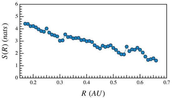
Figure 5.
Behavior of the Shannon entropy of the filtered normal component of the magnetic field as a function of the radial distance R from the Sun.
Indeed, since the magnetic field magnitude is decreasing with the distance also the magnetic energy should be a decreasing function of R. However, by evaluating the behavior of the Shannon entropy as a function of (see Figure 6), we clearly note a logarithmic dependence between the Shannon entropy and the mean squared value of the filtered normal component, i.e., .
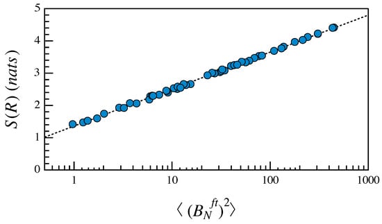
Figure 6.
The Shannon entropy of the filtered normal component of the magnetic field versus the mean squared value of the filtered normal component.
As a consequence of the previous considerations in order to evaluate the real evolution of the entropy and the relative degree of self-organization (degree of order) as a function of the radial distance R, we need to apply the Klimontovich S-theorem. First of all, we have to choose the reference state by a pairwise comparison between states using Equation (17). Figure 7 shows the disorder matrix computed as described in Section 3.2 using the distribution functions, and , for each couple of different distributions.
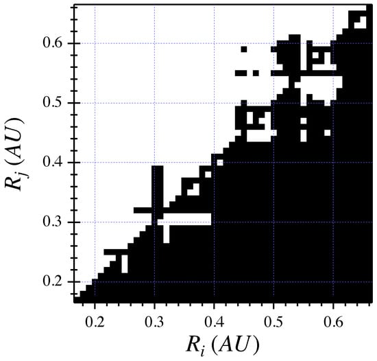
Figure 7.
The disorder matrix . Here, black color refers to and white color to .
According to the disorder matrix , the state associated with the maximum disorder is the one corresponding to the maximum distance explored by PSP, being . Thus, in analysing the degree of self-organization using the Klimontovich S-theorem, we have set as reference state “0” the one at the maximal distance, i.e., the one at AU.
Figure 8 shows the results of the Klimontovich S-theorem analysis in terms of effective temperature as a function of the radial distance R from the Sun. The shows a decrease with the distance from the Sun, indicating that the fluctuations of the normal component in the inertial range show an increase of the degree of self-organization moving towards the Sun. In other words, we should expect that there is an increase of the entropic character of the fluctuations with the radial distance R. In particular, all the states associated with a radial distance less than the reference state show an effective temperature , supporting the hypothesis that the fluctuations at lower distances from the Sun are characterized by a higher degree of self-organization according to S-theorem.
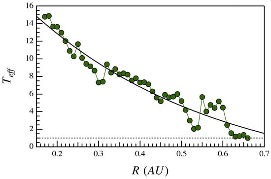
Figure 8.
The effective temperature as a function of the radial distance R from the Sun. Solid line is an eye-guide. The horizontal dashed line refers to the critical value .
Figure 9 reports the behavior of the entropy reduction/variation as a function of the radial distance R. Entropy reduction/variation decreases with the radial distance, indicating that, in spite of the higher absolute value of the entropy observed in Figure 5 closer to the Sun, the fluctuations at inner distances are less entropic once the entropy is renormalized to take into account the total energy of the system. Furthermore, the behavior of the seems to follow a sigmoid shape (Hill function), suggesting the existence of a transition region approximately at AU.
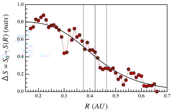
Figure 9.
The behavior of the entropy reduction/variation as a function of the radial distance R. Solid line is best fit using the Hill function. The vertical solid and dashed lines refer to the transition region AU.
Looking to the trend of , we can observe how there is a clear difference between inner heliospheric regions ( AU) and outer ones, where the inner region fluctuations show a less entropic and more self-organized character. The observed change in the entropic nature of fluctuations suggests the occurrence of a dynamical phase transition in the fluctuation field with the radial distance.
We notice how the observed transition region is well in agreement with previous findings by Chen et al. [21] and Alberti et al. [22] that have observed changes in several physical quantities (normalized cross-helicity, Alfvénicity, spectral features, scaling exponents and multifractal spectral widths ) in the same distance interval.
5. Discussions
Here, we have investigated the dependence of the degree of self-organization by means of Klimontovich S-theorem using, as a control parameter, the radial distance R from the Sun. As already mentioned above, R is clearly not the relevant physical quantity in forcing self-organization, being, indeed, a simple parameter that can be used to study the fluctuation field evolution. Thus, in what follows, we attempt to correlate the observed dynamical evolution with some physical quantities. Among the different physical quantities investigated in the recent literature [21,22], one of the most promising quantities that could be responsible for the order-disorder transition observed as a function of the radial distance, is the magnetic field intensity. Indeed, as well as reported in the literature [38], a strong magnetic field in a specific direction, could inhibit fluctuations in that direction. Thus, we can expect that the features of fluctuation field could strongly depend on the magnetic field intensity.
Figure 10 shows the behavior of the effective temperature in comparison with the average magnetic field intensity . Both the quantities show a similar trend, i.e., a decreasing with the radial distance, suggesting that there could be a relationship between the two quantities. This relation is clear by plotting versus (see Figure 11). In fact, the degree of self-organization as measured by the effective temperature linearly scales with the logarithm of the magnetic field intensity (Pearson’s ). This clear relationship between and supports the hypothesis that magnetic field intensity plays a relevant role in increasing the degree of order of fluctuations of the magnetic field. The plays the role of a control parameter.
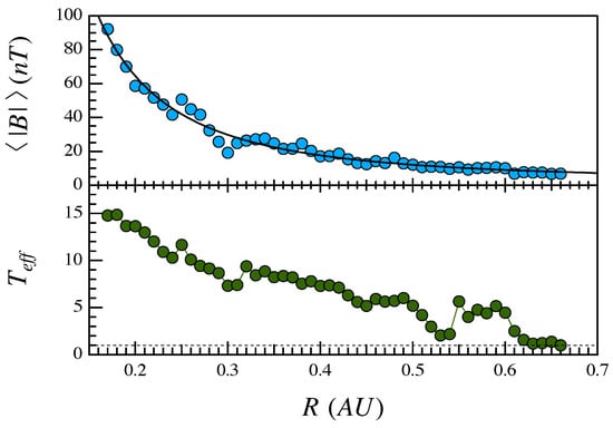
Figure 10.
The trend behavior of the effective temperature (bottom panel) in comparison with the average magnetic field intensity (up panel).
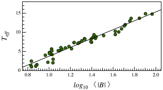
Figure 11.
The effective temperature versus . The solid line is a linear fit.
To verify the above hypothesis, we plot the entropy reduction/variation vs. in Figure 12. A clear continuous dependence of the entropy reduction/variation as a function of the is found, supporting that the last quantity plays the role of the control parameter. Furthermore, the observed trend of as a function of the is the signature of the occurrence of a phase transition. This transition resembles the typical behavior of a continuous phase transition where the is the control parameter.
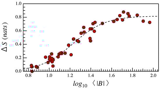
Figure 12.
The entropy reduction/variation versus . The dashed curve is a sigmoid fit of the data.
Resuming our findings, the observed (dynamical) phase transition seems to occur in correspondence of a value of the magnetic field intensity of the order of nT, which corresponds to a radial distance AU from the Sun. This distance agrees with both the previous findings and the results by recent works on different quantities [21,22].
6. Summary and Conclusions
In this work, we have investigated the occurrence of a nonequilibrium phase transition in the inertial range fluctuation field of IMF as a function of the radial distance from the Sun. The motivation for this work can be found in the previous analyses by Chen et al. [21] and Alberti et al. [22], which provided an indication for the occurrence of a dynamical change of several physical quantities and properties of the fluctuations in the inertial range. In particular, Chen et al. [21] evidenced how at a distance between 0.3 AU and 0.4 AU, there is a significant reduction of the Alfvénic character of fluctuations, a decrease of the cross-helicity , and a continuous steepening of the magnetic field spectral index with the radial distance from the Sun. Furthermore, Alberti et al. [22] observed a breakdown of the multifractal character of magnetic field fluctuations in the inertial range moving towards the Sun at a distance near 0.4 AU. All these previous features suggest that near 0.4 AU, the solar wind turbulent features can undergo a dynamical phase transition.
Here, we provided evidence of this dynamical phase transition by means of the Klimontovich S-theorem, which allows one to quantify and compute the degree of self-organization between two nonequilibrium stationary states in open systems. Our results suggest that the degree of self-organization, as quantified by the effective temperature , decreases with the radial distance from the Sun. This reduction of the self-organization and relative ordering of the solar wind turbulent fluctuation field with the radial distance was already found in a previous paper by Consolini and de Michelis [39], where a decrease in the degree of order between solar wind turbulence at 1A and 5 AU was observed. This decrease was interpreted as an evidence of decaying turbulence. Conversely, to these results Consolini and de Michelis [39], the observed changes of the degree of order seem to be of a different nature. Indeed, this is accompanied by a continuous change of the entropy reduction , which resembles the typical shape of a continuous transition between two different states. Furthermore, we have found that the magnetic field intensity (or more precisely, ) can play the role of a control parameter. This seems a reasonable quantity which can inhibit some degree of freedom in the system, freezing fluctuations along the magnetic field direction. Apart from the previous considerations and results on the dependence of various quantities on the radial distance [21,22], a possible origin of the observed transition could be a change from a forced turbulence to decaying turbulence, as also observed in simulations of Alfvénic turbulence by Chen et al. [40].
In conclusion, in this work, we have demonstrated the occurrence of a dynamical nonequilibrium phase transition in the solar wind magnetic field fluctuations in the inner heliosphere, suggesting some possible mechanisms that could be responsible for the observed dynamical changes. More work is necessary to better identify the mechanisms responsible for the observed transition.
Author Contributions
Conceptualization, G.C.; Data curation, T.A.; Investigation, M.S., V.Q., S.B., T.A. and G.C.; Methodology, M.S. and V.Q.; Software, M.S.; Writing—original draft, M.S., V.Q., S.B., T.A. and G.C.; Writing—review and editing, M.S., V.Q., S.B., T.A. and G.C. All authors have read and agreed to the published version of the manuscript.
Funding
G.C. and S.B. acknowledge financial support by Italian MIUR-PRIN grant 2017APKP7T on Circumterrestrial Environment: Impact of Sun-Earth Interaction. V.Q. acknowledges the financial support by Italian Space Agency under project Limadou-2 fase B2/C/D/E1 (ASI-INFN n. 2016-4-Q.0 n. 312818).
Institutional Review Board Statement
Not applicable.
Informed Consent Statement
Not applicable.
Data Availability Statement
Not applicable.
Acknowledgments
The data used in this study are available at the NASA Space Physics Data Facility (SPDF), https://spdf.gsfc.nasa.gov/index.html (accessed on 8 February 2021). The authors acknowledge the contributions of the FIELDS team to the Parker Solar Probe mission. M.S. acknowledges the PhD course in Astronomy, Astrophysics and Space Science of the University of Rome “Sapienza University of Rome”, University of Rome “Tor Vergata” and National Institute of Astrophysics (INAF), Italy. V.Q. acknowledges the PhD Program in Physics and Chemistry of the University of L’Aquila (Italy). T.A. and G.C. acknowledge fruitful discussions within the scope of the International Team “Complex Systems Perspectives Pertaining to the Research of the Near-Earth Electromagnetic Environment” at the International Space Science Institute in Bern, Switzerland.
Conflicts of Interest
The authors declare no conflict of interest.
Abbreviations
The following abbreviations are used in this manuscript:
| AU | Astronomical Unit |
| IMF | Interplanetary Magnetic Field |
| PSP | Parker Solar Probe |
References
- Valentini, F.; Califano, F.; Veltri, P. The kinetic nature of turbulence at short scales in the solar wind. Planet. Space Sci. 2011, 59, 547–555. [Google Scholar] [CrossRef]
- Bruno, R.; Carbone, V. Turbulence in the Solar Wind; Springer: Berlin/Heidelberg, Germany, 2016; Volume 928. [Google Scholar]
- Verscharen, D.; Klein, K.G.; Maruca, B.A. The multi-scale nature of the solar wind. Living Rev. Sol. Phys. 2019, 16, 5. [Google Scholar] [CrossRef] [PubMed]
- Matsumoto, T. Full compressible 3D MHD simulation of solar wind. Mon. Not. R. Soc. 2021, 500, 4779–4787. [Google Scholar] [CrossRef]
- Macek, W.M.; Wawrzaszek, A.; Carbone, V. Observation of the multifractal spectrum in the heliosphere and the heliosheath by Voyager 1 and 2. J. Geophys. Res. (Space Phys.) 2012, 117, A12101. [Google Scholar] [CrossRef]
- Carbone, V. Scalings, Cascade and Intermittency in Solar Wind Turbulence. Space Sci. Rev. 2012, 172, 343–360. [Google Scholar] [CrossRef]
- Sorriso-Valvo, L.; Carbone, V.; Giuliani, P.; Veltri, P.; Bruno, R.; Antoni, V.; Martines, E. Intermittency in plasma turbulence. Planet. Space Sci. 2001, 49, 1193–1200. [Google Scholar] [CrossRef]
- Sorriso-Valvo, L.; De Vita, G.; Fraternale, F.; Gurchumelia, A.; Perri, S.; Nigro, G.; Catapano, F.; Retinò, A.; Chen, C.H.K.; Yordanova, E.; et al. Sign singularity of the local energy transfer in space plasma turbulence. Front. Phys. 2019, 7, 108. [Google Scholar] [CrossRef]
- Martinović, M.M.; Klein, K.G.; Bourouaine, S. Radial Evolution of Stochastic Heating in Low-β Solar Wind. Astrophys. J. 2019, 879, 43. [Google Scholar] [CrossRef]
- Marsch, E. Solar wind and kinetic heliophysics. Ann. Geophys. 2018, 36, 1607–1630. [Google Scholar] [CrossRef]
- Lepping, R.P.; Acũna, M.H.; Burlaga, L.F.; Farrell, W.M.; Slavin, J.A.; Schatten, K.H.; Mariani, F.; Ness, N.F.; Neubauer, F.M.; Whang, Y.C.; et al. The Wind Magnetic Field Investigation. Space Sci. Rev. 1995, 71, 207–229. [Google Scholar] [CrossRef]
- Lin, R.P.; Anderson, K.A.; Ashford, S.; Carlson, C.; Curtis, D.; Ergun, R.; Larson, D.; McFadden, J.; McCarthy, M.; Parks, G.K.; et al. A Three-Dimensional Plasma and Energetic Particle Investigation for the Wind Spacecraft. Space Sci. Rev. 1995, 71, 125–153. [Google Scholar] [CrossRef]
- Stone, E.C.; Frandsen, A.M.; Mewaldt, R.A.; Christian, E.R.; Margolies, D.; Ormes, J.F.; Snow, F. The Advanced Composition Explorer. Space Sci. Rev. 1998, 86, 1–22. [Google Scholar] [CrossRef]
- Balogh, A.; Carr, C.M.; Acuña, M.H.; Dunlop, M.W.; Beek, T.J.; Brown, P.; Fornaçon, K.H.; Georgescu, E.; Glassmeier, K.H.; Harris, J.; et al. The Cluster Magnetic Field Investigation: Overview of in-flight performance and initial results. Ann. Geophys. 2001, 19, 1207–1217. [Google Scholar] [CrossRef]
- Burch, J.L.; Moore, T.E.; Torbert, R.B.; Giles, B.L. Magnetospheric Multiscale Overview and Science Objectives. Space Sci. Rev. 2016, 199, 5–21. [Google Scholar] [CrossRef]
- Fox, N.J.; Velli, M.C.; Bale, S.D.; Decker, R.; Driesman, A.; Howard, R.A.; Kasper, J.C.; Kinnison, J.; Kusterer, M.; Lario, D.; et al. The Solar Probe Plus Mission: Humanity’s First Visit to Our Star. Space Sci. Rev. 2016, 204, 7–48. [Google Scholar] [CrossRef]
- Velli, M.; Harra, L.K.; Vourlidas, A.; Schwadron, N.; Panasenco, O.; Liewer, P.C.; Müller, D.; Zouganelis, I.; St Cyr, O.C.; Gilbert, H.; et al. Understanding the origins of the heliosphere: Integrating observations and measurements from Parker Solar Probe, Solar Orbiter, and other space- and ground-based observatories. Astron. Astrophys. 2020, 642, A4. [Google Scholar] [CrossRef]
- Dudok de Wit, T.; Krasnoselskikh, V.V.; Bale, S.D.; Bonnell, J.W.; Bowen, T.A.; Chen, C.H.K.; Froment, C.; Goetz, K.; Harvey, P.R.; Jagarlamudi, V.K.; et al. Switchbacks in the Near-Sun Magnetic Field: Long Memory and Impact on the Turbulence Cascade. Astrophys. J. Suppl. Ser. 2020, 246, 39. [Google Scholar] [CrossRef]
- Zank, G.P.; Nakanotani, M.; Zhao, L.L.; Adhikari, L.; Kasper, J. The Origin of Switchbacks in the Solar Corona: Linear Theory. Astrophys. J. 2020, 903, 1. [Google Scholar] [CrossRef]
- Kasper, J.C.; Bale, S.D.; Belcher, J.W.; Berthomier, M.; Case, A.W.; Chandran, B.D.G.; Curtis, D.W.; Gallagher, D.; Gary, S.P.; Golub, L.; et al. Alfvénic velocity spikes and rotational flows in the near-Sun solar wind. Nature 2019, 576, 228–231. [Google Scholar] [CrossRef]
- Chen, C.H.K.; Bale, S.D.; Bonnell, J.W.; Borovikov, D.; Bowen, T.A.; Burgess, D.; Case, A.W.; Chandran, B.D.G.; de Wit, T.D.; Goetz, K.; et al. The Evolution and Role of Solar Wind Turbulence in the Inner Heliosphere. Astrophys. J. Suppl. Ser. 2020, 246, 53. [Google Scholar] [CrossRef]
- Alberti, T.; Laurenza, M.; Consolini, G.; Milillo, A.; Marcucci, M.F.; Carbone, V.; Bale, S.D. On the Scaling Properties of Magnetic-field Fluctuations through the Inner Heliosphere. Astrophys. J. 2020, 902, 84. [Google Scholar] [CrossRef]
- Kolmogorov, A. The Local Structure of Turbulence in Incompressible Viscous Fluid for Very Large Reynolds’ Numbers. Akad. Nauk SSSR Dokl. 1941, 30, 301–305. [Google Scholar]
- Kraichnan, R.H. Inertial-Range Spectrum of Hydromagnetic Turbulence. Phys. Fluids 1965, 8, 1385–1387. [Google Scholar] [CrossRef]
- Frisch, U. From global scaling, a la Kolmogorov, to local multifractal scaling in fully developed turbulence. Proc. R. Soc. Lond. Ser. A 1991, 434, 89–99. [Google Scholar] [CrossRef]
- Katul, G.G.; Parlange, M.B.; Chu, C.R. Intermittency, local isotropy, and non-Gaussian statistics in atmospheric surface layer turbulence. Phys. Fluids 1994, 6, 2480–2492. [Google Scholar] [CrossRef]
- Dubrulle, B. Beyond Kolmogorov cascades. J. Fluid Mech. 2019, 867, P1. [Google Scholar] [CrossRef]
- Donner, R.V.; Zou, Y.; Donges, J.F.; Marwan, N.; Kurths, J. Recurrence networks—A novel paradigm for nonlinear time series analysis. New J. Phys. 2010, 12, 033025. [Google Scholar] [CrossRef]
- Alberti, T.; Consolini, G.; Carbone, V.; Yordanova, E.; Marcucci, M.; De Michelis, P. Multifractal and Chaotic Properties of Solar Wind at MHD and Kinetic Domains: An Empirical Mode Decomposition Approach. Entropy 2019, 21, 320. [Google Scholar] [CrossRef]
- Alberti, T.; Consolini, G.; Carbone, V. A discrete dynamical system: The poor man’s magnetohydrodynamic (PMMHD) equations. Chaos 2019, 29, 103107. [Google Scholar] [CrossRef]
- Donner, R.V.; Heitzig, J.; Donges, J.F.; Zou, Y.; Marwan, N.; Kurths, J. The geometry of chaotic dynamics—A complex network perspective. Eur. Phys. J. B 2011, 84, 653–672. [Google Scholar] [CrossRef]
- Klimontovich, Y. Statistical Theory of Open Systems; Kluwer Academic Pub.: Dordrecht, The Netherlands, 1995; Volume 1. [Google Scholar]
- Klimontovich, Y. Entropy evolution in self-organization process H-theorem and S-theorem. Phys. A Stat. Mech. Its Appl. 1987, 142, 390–404. [Google Scholar] [CrossRef]
- Van Kampen, N. The definition of entropy in non-equilibrium states. Physica 1959, 25, 1294–1302. [Google Scholar] [CrossRef]
- Bale, S.D.; Goetz, K.; Harvey, P.R.; Turin, P.; Bonnell, J.W.; Dudok de Wit, T.; Ergun, R.E.; MacDowall, R.J.; Pulupa, M.; Andre, M.; et al. The FIELDS Instrument Suite for Solar Probe Plus. Measuring the Coronal Plasma and Magnetic Field, Plasma Waves and Turbulence, and Radio Signatures of Solar Transients. Space Sci. Rev. 2016, 204, 49–82. [Google Scholar] [CrossRef] [PubMed]
- Mariani, F.; Ness, N.F.; Burlaga, L.F.; Bavassano, B.; Villante, U. The large-scale structure of the interplanetary magnetic field between 1 and 0.3 AU during the primary mission of Helios 1. J. Geophys. Res. Space Phys. 1978, 83, 5161–5166. [Google Scholar] [CrossRef]
- Parker, E.N. Dynamics of the Interplanetary Gas and Magnetic Fields. Astrophys. J. 1958, 128, 664. [Google Scholar] [CrossRef]
- Biskamp, D. Magnetohydrodynamic Turbulence; Cambridge University Press: Cambridge, UK, 2003. [Google Scholar]
- Consolini, G.; de Michelis, P. Relative ordering in the radial evolution of solar wind turbulence: The S-Theorem approach. Ann. Geophys. 2011, 29, 2317–2326. [Google Scholar] [CrossRef]
- Chen, C.H.K.; Mallet, A.; Yousef, T.A.; Schekochihin, A.A.; Horbury, T.S. Anisotropy of Alfvénic turbulence in the solar wind and numerical simulations. Mon. Not. R. Astron. Soc. 2011, 415, 3219–3226. [Google Scholar] [CrossRef]


Publisher’s Note: MDPI stays neutral with regard to jurisdictional claims in published maps and institutional affiliations. |
© 2021 by the authors. Licensee MDPI, Basel, Switzerland. This article is an open access article distributed under the terms and conditions of the Creative Commons Attribution (CC BY) license (http://creativecommons.org/licenses/by/4.0/).