Article

Quantifying the Impact of the Covid-19 Lockdown Measures on Nitrogen Dioxide Levels throughout Europe

Norwegian Institute for Air Research, Instituttveien 18, 2007 Kjeller, Norway
*
Author to whom correspondence should be addressed.
Atmosphere 2021, 12(2), 131; https://doi.org/10.3390/atmos12020131
Submission received: 21 December 2020 / Revised: 12 January 2021 / Accepted: 18 January 2021 / Published: 20 January 2021
(This article belongs to the Section Air Quality)

Abstract

:
In this paper, the effect of the lockdown measures on nitrogen dioxide (NO2) in Europe is analysed by a statistical model approach based on a generalised additive model (GAM). The GAM is designed to find relationships between various meteorological parameters and temporal metrics (day of week, season, etc.) on the one hand and the level of pollutants on the other. The model is first trained on measurement data from almost 2000 monitoring stations during 2015–2019 and then applied to the same stations in 2020, providing predictions of expected concentrations in the absence of a lockdown. The difference between the modelled levels and the actual measurements from 2020 is used to calculate the impact of the lockdown measures adjusted for confounding effects, such as meteorology and temporal trends. The study is focused on April 2020, the month with the strongest reductions in NO2, as well as on the gradual recovery until the end of July. Significant differences between the countries are identified, with the largest NO2 reductions in Spain, France, Italy, Great Britain and Portugal and the smallest in eastern countries (Poland and Hungary). The model is found to perform best for urban and suburban sites. A comparison between the found relative changes in urban surface NO2 data during the lockdown and the corresponding changes in tropospheric vertical NO2 column density as observed by the TROPOMI instrument on Sentinel-5P revealed good agreement despite substantial differences in the observing method.

1. Introduction

The global Covid-19 pandemic in 2020 has led to major changes in society, the economy, and transportation worldwide. In Europe, the first cases of Covid-19 were detected by the end of January. In February, the number of incidents increased substantially in a few countries—Italy, France and Spain—and Italy was the first country in Europe to introduce restrictions on the population. Italy imposed a quarantine on more than 50,000 people in the northern part of the country on 22 February.
During March, most European countries introduced a full national lockdown, and most of these actions were taken mid-month. By 18 March, more than 250 million people were in lockdown in Europe, and by the beginning of April, 3.9 billion people or around half the global population were subject to complete or partial lockdown [1]. The global road transport activity was almost 50% below the 2019 average by the end of March, and commercial flight activity nearly 75% below 2019 by mid-April 2020 [2]. The lockdown restrictions were gradually lifted in the following weeks and months, varying substantially between the countries in Europe.
The reduced road transport and aviation led to reduced emissions of air pollutants and thereby lower levels of atmospheric pollutants, as documented by several European studies [3,4,5,6,7,8,9,10,11]. The quantification of this effect is, however, not trivial. First, weather patterns have a decisive influence on air pollutants’ concentration through atmospheric mixing and wash-out of aerosols by precipitation. Dacre et al. [5] showed that meteorology changes from pre- to post-lockdown periods in the UK counteracted the effect of reduced NOx emissions. Second, the onset of the lockdown was in spring, which typically is a transition period associated with marked changes in the prevailing pollutant levels. Peak levels of primary pollutants, such as NO2, are typically observed in winter during episodes of low temperatures and inefficient atmospheric mixing. In contrast, secondary pollutants, such as O3 and organic aerosols, peak in summer. Finally, an assessment of the lockdown effect on the pollutant levels should also consider the year-by-year downward trend in pollutants due to policy-driven emission abatement actions in Europe.
Several hundred journal articles have already been published on the link between the Covid-19 lockdown and reduced air pollution in Europe and other regions. The publications can be divided into three categories:
  • Pure observational-based studies in which the lockdown periods are compared with non-lockdown periods [3,10,12], either using measurements from previous years or by looking at pre- and post-lockdown periods in 2020.
  • Studies based on chemical transport models (CTMs) and observations in combination [4,7,8,13,14,15,16,17] either by running separate baseline and lockdown emission scenarios or by estimating the lockdown effect from a comparison between measurements and business-as-usual scenarios.
  • Statistical based studies [5,6,9,18] using multiple regression, generalised additive model (GAM), or machine learning (ML) models to estimate the links between measured concentration levels and meteorological as well as time (day of week, etc.) data. Some studies also use a combination of statistical methods and CTMs [4,7].
There are pros and cons to each of these approaches. Pure observational-based studies are easy to conduct and avoid all model assumptions but are hampered by difficulties in subtracting the meteorological impact. CTM based studies are the standard way of assessing air pollution levels, but for the lockdown period, the CTMs were faced with difficulties with the emission scenarios since the emission changes during lockdown will vary with city, country and time. Some CTM studies use activity data during the lockdown as a proxy for the emissions [8]. In contrast, others use country- and sector-resolved emission reduction factors [4], and some studies have even turned off emissions from specific sectors entirely [16].
An advantage of statistical models (compared to CTMs) is that they do not require any emissions assumptions. Furthermore, as opposed to CTMs, statistical models can be trained on data for each measurement station separately to give optimal prediction accuracy for every station. This is particularly important for, e.g., traffic sites since concentration levels at such locations can deviate quite substantially from the surrounding grid concentrations. The main disadvantage of statistical models vs. a CTM is that the former is not built as a physical causal model but only uses statistically found associations between a set of explanatory meteorological and time variables and the resulting concentrations. Thus, one should be careful with extrapolating results from such a model to other sites and periods far into the past or future.
In this paper, we show that a specific type of statistical regression model, namely a generalised additive model (GAM), is particularly well suited for isolating the effect of the reduced emissions from other confounding processes. Various studies using machine-learning (ML) methods have been used to assess the lockdown effect on air pollutants, and the gradient boosting technique has been particularly popular [4,7,9]. The GAM approach [19,20] can also be considered an ML method. Still, the main advantage of a GAM model lies in its interpretability. It provides direct functional relationships between each input explanatory variable and the response variable (the atmospheric concentration). In contrast, other ML methods are less interpretable and tend to produce more “black-box” non-transparent relationships and results. The GAM modelling approach is also often found to have good predictive abilities [20,21].
Furthermore, since the GAM model is statistical in nature, we can provide 95% uncertainty intervals for the model predictions, which enable us to compare and check the resulting accuracy of the model with the actual observations. The GAM model can also estimate and consider long-term trends in the concentration levels over several years in the predictions for a left-out or future year without any assumptions about the change in emissions with time. The present study is a substantial extension of the preliminary results presented in [11].
Despite the fundamental differences between the various methodologies discussed above, the estimated effects of lockdown on NO2 levels in Europe seem to be reasonably consistent across the studies. The studies are, however, not directly comparable since the studied periods differ somewhat.
In their observational-based work, Baldasano [3], Sicard et al. [10], and Tobias et al. [12] all estimated reductions in the NO2 concentration levels of the order of 50–65% for urban and traffic sites in Spain, France and Italy in March 2020. They also found that consideration of the varying weather patterns had a decisive influence on the estimated levels. These estimations agree very well with the CTM based findings of [4] for urban areas in the same countries. For countries that adopted softer lockdown measures, such as Germany, the Netherlands, Poland and Sweden, Barré et al. [4] estimated smaller reductions in NO2 levels. Keller et al. [7], using the NASA global atmospheric composition model GEOS-CF (GEOS Composition Forecasts) with a bias-correction methodology found a 46% reduction in NO2 over Spain (14 March to 23 April) and widespread reductions in the order of 22% in March and 33% in April over Europe. Using the WRF-CHIMERE model for Western Europe with different emission scenarios, Menut et al. [8] estimated NO2 concentration reductions in the order of 15–30% for Germany and the Netherlands and 35–45% on average in other countries for March 2020. Grivas et al. [13], looking at the Greater Athens area using the TAPM model estimated average NO2 concentration reductions in 30–35%, and up to 50% reduction in some Athens basin areas.
Based on a machine learning model fed by meteorological data and time features for background and traffic stations in Spain, Petetin et al. [9] estimated a mean reduction in NO2 concentration levels of 40% already early in the year when less stringent restrictions were introduced, increasing up to 55% reduction during later and more strict phases of the lockdown. Ordonez et al. [18], applying a GAM model for the period 15 March to 30 April found the best correlation for Benelux sites. For the meteorologically adjusted changes, they found 47–50% reductions in the NO2 concentration levels for urban locations in France, Italy and Spain. Grange et al. [6] used an ML model called Random Forest Model on NO2 and O3 data for 102 metropolitan areas and 34 countries in Europe. They estimated NO2 reductions that agree very well with the studies mentioned above, with on average 34 and 32% lower concentration levels than expected at traffic/roadside sites and urban background sites, respectively. They also found that the oxidant level (Ox = NO2 + O3) was more or less unchanged during the lockdown, implying a similar increase in O3 accompanied the reduced NO2.

2. Method

A GAM model [19,20] is a non-linear regression model linking expected values μ i of a given response variable Y i to several explanatory variables x i j through the following set of relations:
g ( μ i ) = β 0 + j = 1 p β j ( x i j ) ; μ i = E ( Y i )
where β 0 is a constant (the intercept), and where β j ( ) , for j = 1 , , p , represents smooth functions of the covariates x i j , with p the number of such covariates.
Our GAM model was developed over several years [22,23] and was initially designed to assess air pollutant trends in Europe based on long-term monitoring data of O3, NO2 and PM. That work aimed to apply and adapt for European conditions a statistical method that has been used by the US-EPA (Environmental Protection Agency) on a routine basis for surface ozone trend assessments, adjusting for the inter-annual impact of changing meteorology [24].
The response variable Y i in (Equation (1)) represents a measured air pollutant concentration at day number i at a given site, while x i j represents the values of individual explanatory variables for j = 1 , , p at the same location and at the same day i , typically meteorological data, such as temperature, humidity, etc., as well as time variables (day of the week, etc.). In (Equation (1)) g ( ) is a function linking the statistical expected value of the response variable Y i , i.e., μ i , to the explanatory variables x i j .
In a GAM model, the response variable Y i is assumed to have a specific probability distribution, known as the response distribution, with mean μ i and variance V i . Further, a GAM model is an extension of a multiple linear regression (MLR) model where each β j is a smooth function of x i j and not a constant to be multiplied with x i j as in an MLR model, and where the mean value μ i is more generally related to the covariates through the given link function g ( μ i ) . For NO2, we apply a log link function g ( μ ) = log μ and a Gamma distribution as a response distribution. This is because NO2 has a relatively large range of concentration variation of several orders of magnitude, where the variance of Y i , i.e., V i , is typically proportional to μ i 2 . Thus, for such a variable, it is common practice in GAM modelling to choose a logarithmic link function and a distribution which is skewed to the right, such as a Gamma distribution, as a response distribution for Y i [20]. This was also applied in the previous trend studies [22,23]. In these studies, we looked at surface data of O3, NO2, PM10 and PM2.5.
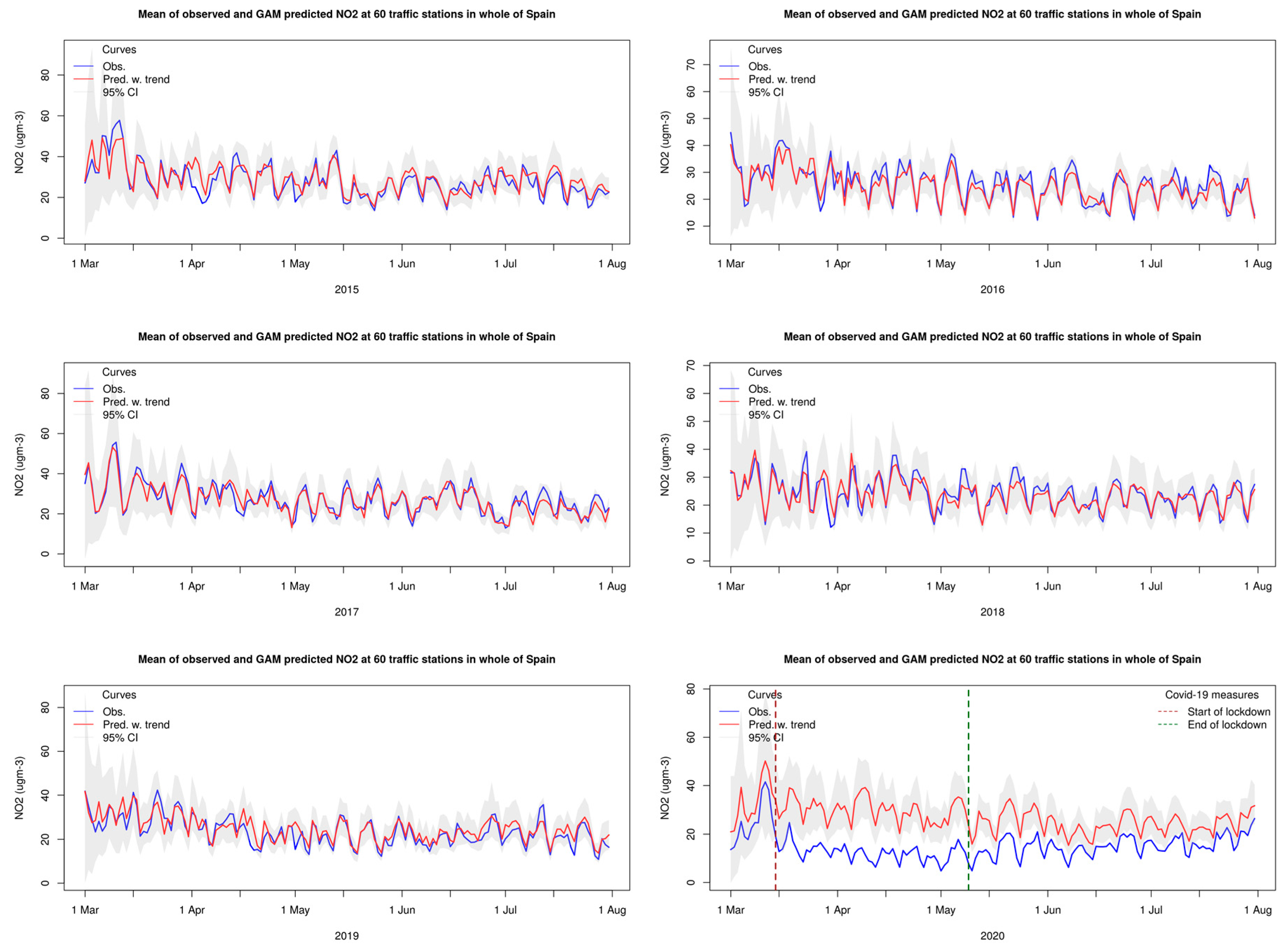
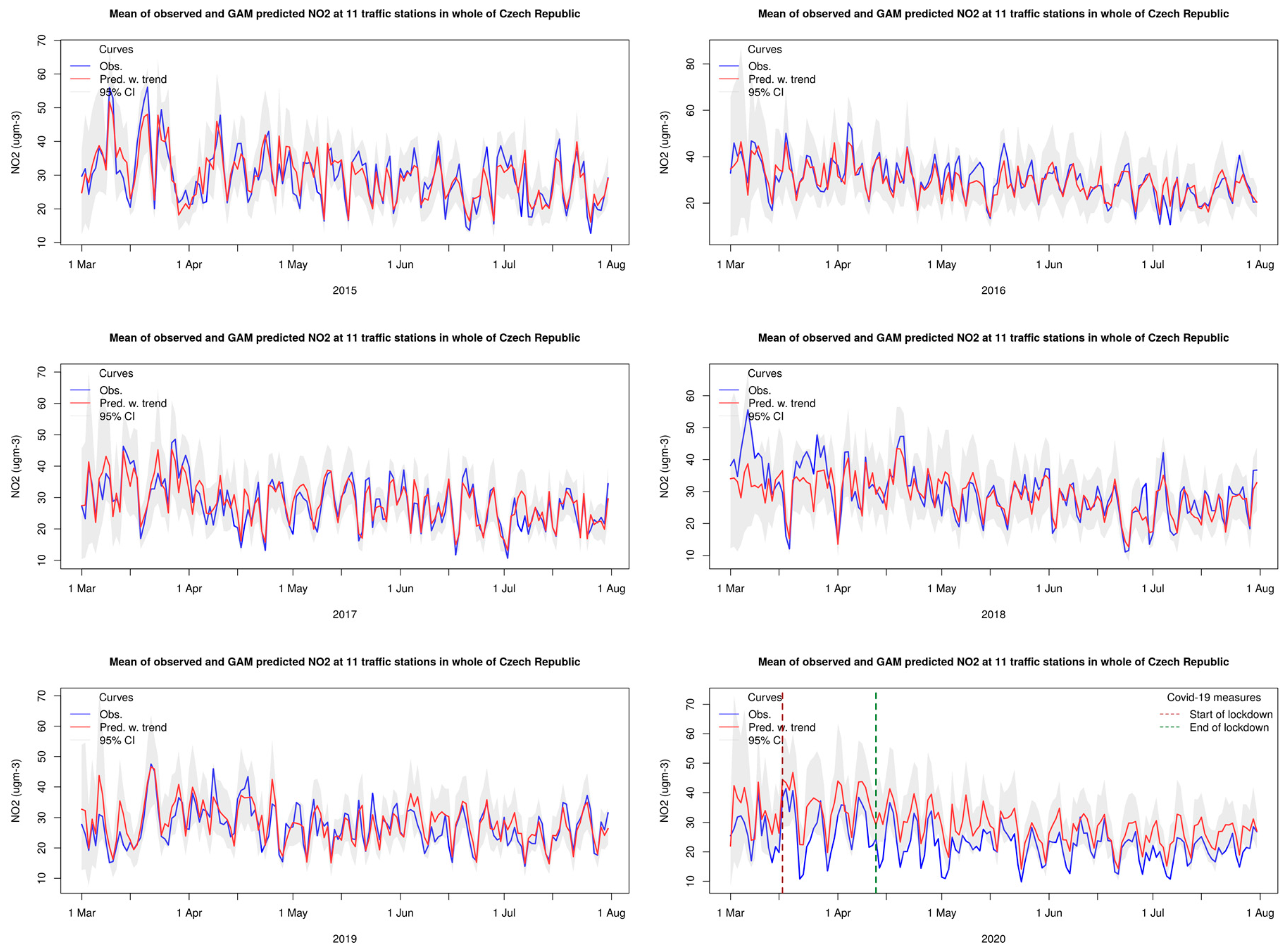
Although developed initially for long-term trend studies, the GAM model proved to be very well suited for studies of the effect of the lockdown measures on air pollutant concentrations during the Covid-19 pandemic. The conceptual idea of the GAM is to establish statistical relationships between the input explanatory variables and the measured air pollutant by training the model on specific periods and then applying the established model to predict the air concentrations in another period. Provided that the model performs reasonably well compared to measurement data, the difference between the predicted NO2 levels for 2020 (the expected or business as usual (BAU)) and the measured levels gives the reduction in NO2 due to the activity restrictions during the pandemic. In the following, we document that the model could be used in this way.

2.1. Statistical Uncertainty of the GAM Predictions

The uncertainty in the GAM model predictions, depicted as the grey shaded areas of the prediction plots in Section 3, is defined as 95% prediction intervals of the unconditional response distribution of modelled concentrations of NO2 for each day. These distributions cannot be given analytically, so a Monte Carlo approach was used to define each interval. At day number i , N samples of log-expected values log μ ^ i j , j = 1 , , N , were first drawn from a normal distribution with mean μ ^ i and standard deviation σ ^ i . These values corresponded to the estimate of the expected value and standard error, respectively, of the linear predictor (Equation (1)) for day number i . Next, shape ( a ) and scale ( s ) parameters of a Gamma conditional response distribution given the expected value μ ^ i j was defined in the usual way [19] as a ^ = ϕ ^ 1 and s ^ = s ^ i j = μ ^ i j / a ^ , where, ϕ ^ is the estimated scale or dispersion parameter. Then, N samples of predicted concentrations y ^ i j were obtained by random draws from Gamma distributions, i.e., y ^ i j Gamma ( a ^ , s ^ i j ) , representing samples from the unconditional (compound) response distribution of modelled concentrations given the data. Finally, a 95% prediction interval was obtained for each day as the interval between the 0.025 and 0.975 sample quantiles of these concentrations. After some testing with various values of N , 100 samples were found to give satisfactory results in defining the 95% prediction intervals, with a good balance between the accuracy of final intervals and the computational efforts.

2.2. Input Data

The study was based on official air quality measurement data reported to the European Environment Agency (EEA) through the e-Reporting system. These data are publicly available through a web interface (https://discomap.eea.europa.eu/map/fme/AirQualityExport.htm). EU member states, EEA countries, and other associated European countries report measurement data for a wide range of air pollutants to EEA’s e-Reporting database on an automated, near real-time basis. The most recent data belong to the E2a data set, also named UTD data (Up to Date), and have been through less stringent quality control procedures. In October/November of each year, the previous year’s data are resubmitted. These data constitute the E1a data set, meaning validated data that have been through more rigorous quality control.
In this study, we investigated the period March–July for the years 2015 through 2020. Measurement data were extracted from the e-Reporting database at the end of October 2020, meaning that we used E1a data for 2015–2018 and many of the sites in 2019 (while E2a for the rest) and E2a data for 2020. March through July 2020 included the introduction of lockdown measures in most of Europe, with substantial implications for the road traffic, particularly in March through April, followed by a period of gradual recovery towards more average conditions. From experience with previous testing and application of the GAM model, the five preceding years (2015–2019) provide a sufficient reference for the GAM to be trained on. A more extended period would reduce the number of available sites and increase the importance of interannual trends in pollutant concentrations, whereas the benefit concerning improved model performance is expected to be minor.
All NO2 data are reported to EEA as hourly averages. The GAM is based on daily input values for meteorology and air quality data, and all NO2 data were transformed to daily mean values on the input to the model.
The monitoring sites reporting to the EEA are classified according to station type (background, industry, or traffic) and area type (rural, suburban, or urban). In principle, this constitutes nine combinations overall, although some combinations will rarely occur (such as background traffic). Based on these classes, we allocated the stations to the following three categories:
  • Traffic (all area types);
  • Urban background and suburban background;
  • Rural background.
We used operational and ERA-interim data [25] for the meteorological input to the model provided by the European Center for Medium-Range Weather Forecast (ECMWF). ERA-interim (ECMWF Re-Analysis) data has a spatial resolution of approximately 0.75°. The operational data, which were used after August 2018 when there was no ERA-interim data available, has a spatial resolution of roughly 0.14°. ERA-interim has 60 vertical levels, and the operational dataset has 137. All data were interpolated from the original data, given as spherical harmonic coefficients to gridded fields of 0.3° resolution.
The input meteorological data are listed in Table 1. Air temperature at 2 m, specific humidity, and the two horizontal wind vectors were extracted from the analysis at 00:00, 06:00, 12:00 and 18:00 UT, respectively, for the lowest vertical model level. Air pressure at mean sea level was available as a surface field. The top net solar radiation and the planetary boundary height were extracted at 15:00 UT as forecasted data. The top net solar radiation was the incoming solar radiation minus the outgoing solar radiation (by reflection and scattering from the atmosphere and the surface) at the top of the atmosphere.
Based on the gridded fields of meteorological data, we prepared annual time series containing daily values of temperature, relative humidity, solar radiation, planetary boundary layer height (PBL) and wind speed and wind direction at 10 m height for each station separately by picking the data values in the grid square containing the station. Temperature, relative humidity and wind were aggregated into daily mean values based on the four data values each day. The mean wind direction was obtained using a vector mean. The other parameters were already given as daily data, as mentioned.
In addition to the meteorological data, three time-variables were included as input to the GAM: day of week number (1, …, 7), the day number in season, and overall time since 1 March 2015 given as year fraction. Whereas the two first variables are cyclic, the latter is a continuous term that considers long-term trends in the concentration levels.
To account for missing data, a data capture criterion of 75% each year was applied, meaning that for a station to be included in the analyses, it should have at least 75% valid daily data for the actual period (March–July) for every year from 2015 through 2020.
As explained above, the model setup implies that the response variable, i.e., the daily mean NO2 concentration, was estimated by a linear combination of the meteorological and time variables for that grid square and that day. In other words, air mass history and long-range transport effects were not considered. While this is a significant simplification, experience shows [23] that this simple approach can predict daily mean NO2 levels fairly accurately at many monitoring stations, as discussed in more detail below.

2.3. Model Performance of the GAM

To assess the model performance, the GAM was used to predict the daily NO2 levels at all sites in each of the years 2015–2019. In these calculations, the GAM was optimised based on data from the remaining years (but not 2020), whereas the actual year was not included. These predicted daily values were then compared to the measured data, as explained below.
Various statistical measures were calculated to assess the model performance based on the predicted vs. the measured daily NO2 concentrations at each site individually for the March–July period. Since the GAM was optimised to the observations, the model was unbiased by construction, and the mean bias was indeed found to be close to zero. In this study, we used the linear correlation coefficient (r) and the normalised mean gross error (NMGE) as the model performance measures. The NMGE was chosen since it is a measure of the mean relative deviation of the model from the observed values and is independent of the absolute level of NO2, which is essential considering the large variations in NO2 concentrations over Europe.
The GAM was applied to almost 2000 stations, and in the post-processing of the results, we found that the model failed for a number of the sites. Inspection of the measurement data indicated that major breaks in the time series (e.g., due to station placement changes) either within one year or between the other years was the cause for many of these failures. Thus, a screening of the stations was required, and we decided to set a criterion of a minimum correlation threshold of r ≥ 0.65 for the linear correlation between the daily GAM predictions and the measured data based on all data from 2015–2019 for a station to be included in the analysis. An additional criterion on the NMGE was not considered necessary since the r-criterion also filtered out the sites with the highest NMGE values.
The total number of sites in each category and their average r and NMGE values (before and after the screening of the stations), as well as the percentage fraction of sites fulfilling the r-criterion, is given in Table 2. The best agreement between the GAM predictions and measurements was found at traffic sites followed by the urban and suburban background sites that showed a somewhat poorer agreement. For rural background sites, the model performance was considerably poorer, which was expected since these sites are, to a larger extent, controlled by long-range transport events and not by the local emissions and meteorology at the site.
Table 2 shows that 85% and 81% of the traffic and urban/suburban stations, respectively, fulfilled the r-criterion, whereas only around half the background rural stations passed this criterion. The mean correlation coefficient for all traffic and urban/suburban sites was 0.72–0.73 and the NMGE 20–24% before filtering. After filtering, the mean r value was 0.77 and the NMGE 18–22% for these sites. The r and NMGE values were considerably poorer for rural background sites before filtering. The total number of sites after filtering was 1383.
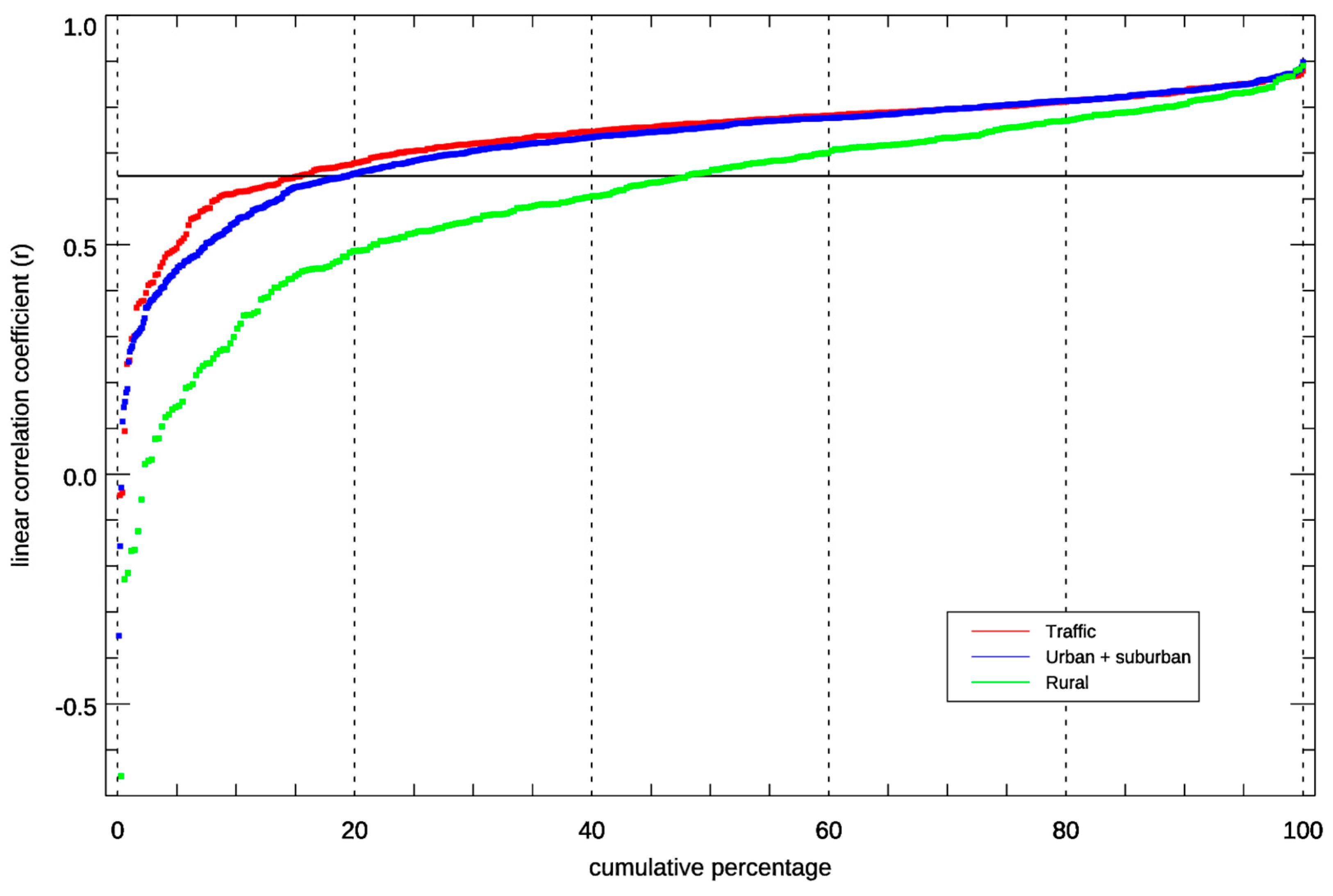
Figure 1 shows the cumulative distribution of the correlation coefficients for the three categories of stations. It indicated that the model performance was fairly even for traffic and urban/sites with a tail of poor-performing sites at the left end of the diagram followed by fairly uniform r values ranging from 0.65–0.90. For the rural background sites, the cumulative distribution was different, indicating that the lack of model performance for these sites reflected that the GAM was less fit to predict NO2 levels at these locations.
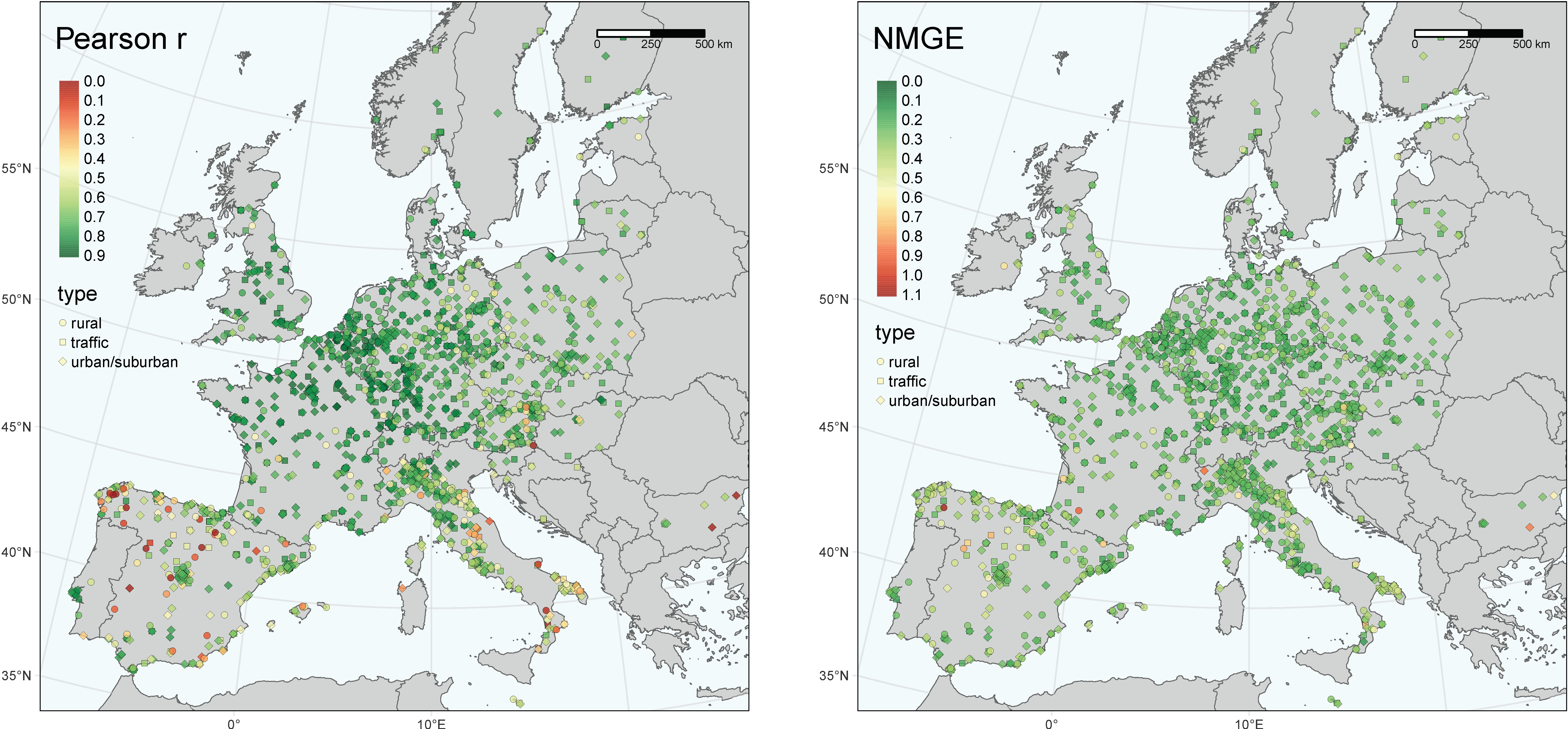
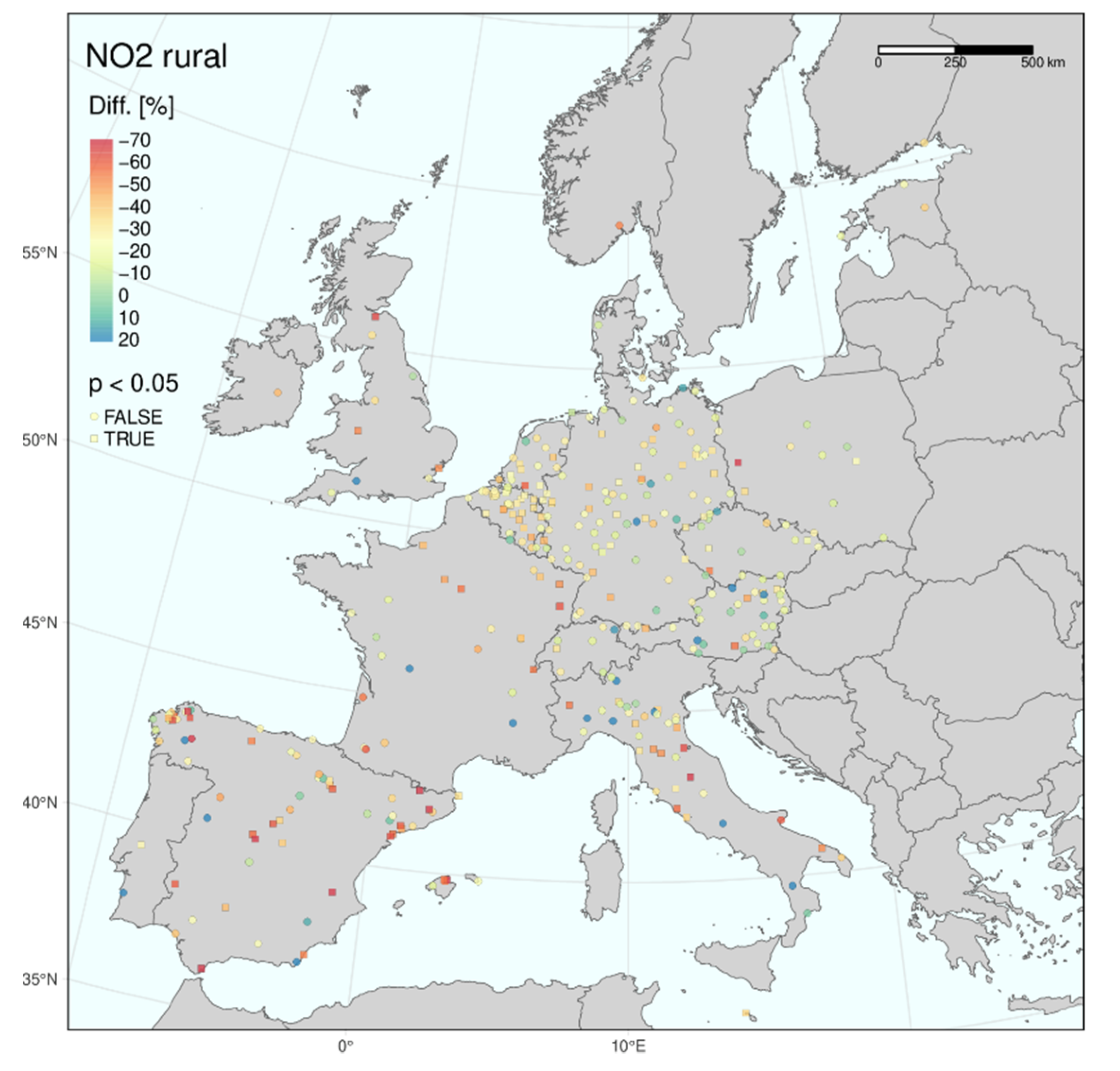
The geographical distribution of r and NMGE for all the NO2 sites before the screening is shown in Figure 2. This indicated that the agreement between the GAM and the measurements was best (high r, low NMGE) in the northwest part of the continent, i.e., Benelux, northwest Germany, northeast France and England. A somewhat more inferior agreement could be observed in southern Europe, particularly Spain and some parts of Italy. 
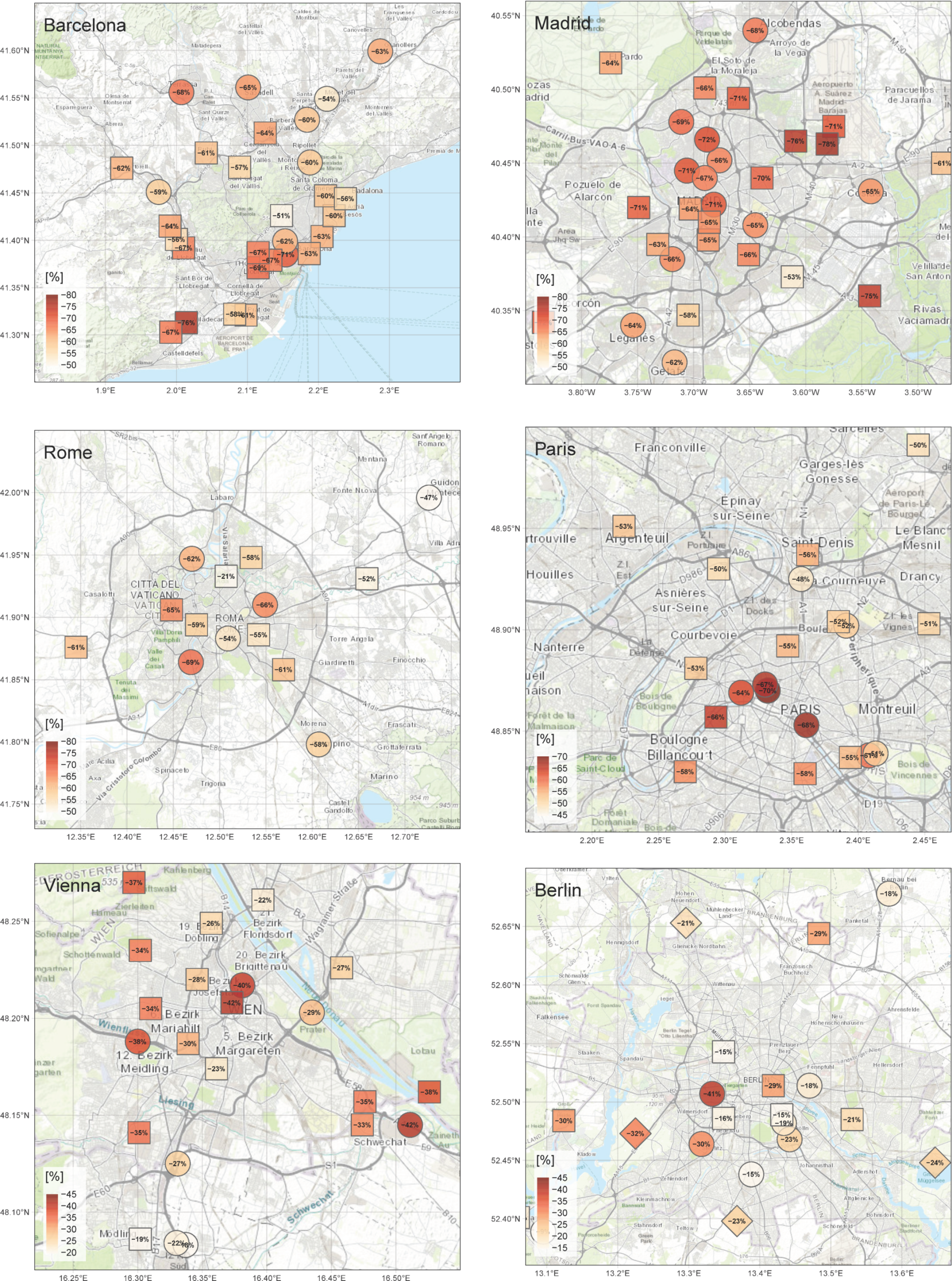
Figure 2 revealed many sites with very low r-value in Spain, mostly at rural background sites. Simultaneously, sites in the Madrid and Barcelona agglomerations showed a good agreement between observed and GAM predicted levels, which are discussed further below.

3. Results and Discussion

3.1. The Impact of Lockdown and Recovery on European NO2 Levels

As explained above, the GAM was first trained on the measured daily data from March–July for the five years 2015–2019 for each monitoring station separately. The estimated GAM model (Equation (1)) was then applied for predicting the expected levels in March–July 2020 given normal conditions and no lockdown. The differences between the GAM model predictions and the measured values are then seen as the effect of the pandemic lockdown restrictions. Only sites fulfilling the criterion of r ≥ 0.65 were included in the following analyses. Figure 3, Figure 4 and Figure 5 show the calculated mean relative differences between the predicted and measured NO2 levels for April 2020, the month with the strongest impact from the lockdown, for the three categories of stations. Stations with a statistically significant change in NO2 (on a p = 0.05 level) were plotted as squares, while the others were plotted as circles.
The results show marked regional differences in Europe, with the most substantial impacts in the south and west and the least impact in the east. These maps indicated that the largest reductions in NO2 levels occurred in Spain, France and Italy and the smallest declines in eastern countries, such as Hungary, Slovakia and Poland.
This is further illustrated in Figure 6, showing the country-averaged spread in the observed minus expected NO2 levels for April in each of the preceding years (2015–2019) given in blue and for April 2020 in red for each country separately. For traffic sites, we estimated the largest median decrease in NO2 levels in Spain (60%), Italy (57%), Portugal (57%), France (56%) and Great Britain (46%). These results agree well with other published studies [4,6,7,8].
These values were calculated as:
Δ N O 2 = N O 2 obs ¯ N O 2 pred ¯ N O 2 pred ¯ × 100 ( % )
where the averages of observed and GAM predicted concentrations were taken over all stations of each category in each country for April in each of the years 2015–2020.
To investigate if the estimated differences in NO2 reductions between the countries could be explained by systematic differences in GAM performance and reflect a model artefact, we looked at the relationship between model performance and ΔNO2. This showed no covariation between the linear correlation coefficients (r) and ΔNO2. Furthermore, the country-wise differences in NO2 concentration reductions during lockdown estimated by our study agrees very well with the results from many other European studies [3,4,6,7,8,18] based on different methodologies. Therefore, we are confident that these differences between the countries express real differences in the lockdown effect on NO2 levels in different countries.
The box-whisker plots shown in Figure 6 are sensitive to outliers when the number of stations is small. This is seen for the traffic sites in Sweden where the results were affected by one single station (SE0058—Dalaplan) in Malmö reporting substantially higher levels than expected in April 2020. These measurements were most likely wrong or reflect a very local change to the traffic pattern since a neighbouring traffic station (SE0096—Bergsgatan) located just 1 km away did not show any signs of such elevated NO2 levels. In addition, in previous years, these two sites were highly correlated with each other.
The initial lockdown effect and the gradual recovery is indicated in Figure 7. This shows the monthly median deviation from the expected NO2 levels, as calculated by the GAM at all urban and suburban stations (including traffic sites) in 2020 for April–July for each country with at least ten such sites. The lockdown was introduced around the middle of March in most countries, whereas lifting the restrictions varied substantially between the countries concerning date and content.
The monthly data given in Figure 7 show a gradual recovery during April–July for all countries. Still, none of the countries was “back to normal” even in July, indicating reduced NO2 levels in all of Europe even long after the lockdown restrictions had been lifted. This agrees with the findings of [7]. Countries in the east with the least reduction in NO2 levels in April, such as Poland and the Czech Republic, also showed the least change during the period, staying at around 20% reduction during these months. In the countries with the largest NO2 reduction in April, the NO2 drop changed in these four months from 60% to 30% in Spain, and from 51% to 19% and 20% in France and Italy, respectively.
The time series of the aggregated NO2 data (observed and predicted) for all traffic stations in Spain and the Czech Republic from 2015 to 2020 is given in Figure 8 and Figure 9 as examples. Similar figures for all countries are given in Figure S1–S3 in the Supplementary Material based on traffic stations, urban/suburban background stations, and rural stations, respectively. These results showed a very good agreement between the observations and the GAM predictions when averaged over the country. The weekly cycle and the peaks and dips through the period were reproduced very satisfactorily by the GAM. The data from the Czech Republic indicated a tendency for an underestimation of the NO2 levels during some of the peak episodes. These results gave strong support that the GAM provides reasonable predictions for the daily NO2 levels at these sites. It should be noted that the model performance was comparable for the other European countries, as can be seen from the plots in the Supplementary Material.
The results for 2020 in Figure 8 show a substantial reduction in measured NO2 levels compared to the Spanish traffic sites’ predictions, most pronounced during the lockdown (14 March–9 May). After lifting the lockdown in May, the disparity between the expected and observed levels was gradually reduced, and by the end of July, the measured NO2 levels were within the 95% confidence interval of the GAM predictions.
In contrast, the results for the Czech traffic sites in 2020 (Figure 9) showed that the measured NO2 levels were below the predictions of the whole period, but mostly within the 95% confidence interval of the predictions and without a very clear trend from March to July, as also discussed above. The country-level differences in the estimated lockdown effects over Europe based on the GAM agree well with other findings as, e.g., reported by [4,7].

3.2. City Level Analysis

Figure 10 shows the observed and predicted NO2 concentrations during March–July at traffic stations in six large cities in Europe: Barcelona, Madrid, Rome, Paris, Vienna and Berlin. For the first four of these cities, the results showed substantial reductions in the NO2 levels compared to the predictions. In contrast, Vienna and Berlin’s levels were only slightly reduced. The Spanish sites’ results align with the study by [10], using an ML-based approach to analyse NO2 data from Spain in March–April.
As seen from Figure 10, the day-to-day variations in the observations follow closely the predictions for all the cities but at lower levels. This is a strong indication that the reduced levels reflect emission reductions and not weather anomalies or other confounding processes. In addition, for Berlin, the observations and predictions correlated very well, indicating that the much smaller reductions in NO2 compared to the other cities reflect that the emission reduction in Berlin during the lockdown was substantially lower than in the other three cities. From 1 May, Berlin’s observed levels were close to the predictions indicating that the road traffic in Berlin was back to normal conditions very early compared to the other cities.
Figure 11 provides a spatial view for the same set of six cities, showing the station-level reductions in measured surface NO2 compared to the business-as-usual scenario.

3.3. A Comparison of the GAM Predictions with Satellite Data for Selected Cities

Earth-observing satellites allow for a unique spatially continuous air quality perspective that is typically not possible with the relatively sparse official air quality monitoring network. The recently launched Sentinel-5P satellite with its TROPOMI instrument allows for maps with higher spatial resolution than previously possible. Using such data, simple comparisons of monthly mean NO2 levels between different years can be made. Figure 12 shows a comparison of the April 2019 NO2 levels against the same period of 2020. Qualitatively, the impact of reduced emissions due to lockdown measures is clearly visible. However, such a simple comparison is prone to various uncertainties, and most importantly, the effect of different meteorology between the two years is not accounted for [4]. Relative differences calculated in such a way between two years result from a combination of various effects and can thus not be interpreted as the sole signal of lockdown measures.
To estimate to what extent quantitative estimates with a simple satellite-based technique are comparable with a more robust meteorology-correcting approach as the one presented in this paper, we extracted the relative difference of the 2019 and 2020 April NO2 Tropospheric Vertical Column Density (TVCD) averages from TROPOMI/S5P over a circular region of 40 km diameter for all cities for which the GAM-based analysis had at least ten stations. All available data from the official Level-2 offline NO2 product were gridded to 0.025° by 0.025° spatial resolution, filtered for clouds and other retrieval issues (using only retrievals with quality assurance flag values of greater than 0.75), averaged to daily mosaics, and subsequently averaged over one month. These non-meteorology-corrected satellite estimates could then be directly compared to the meteorology-corrected relative differences from the GAM approach. The results can be seen in Figure 13. There was a surprisingly strong correlation between the two datasets with an R2 value of 0.91. However, there appeared to be a positive bias in the satellite data, particularly for relative differences around −20%. This was also confirmed by the slope of a linear regression, which showed a slope of 0.81. Nonetheless, the correlation between the two datasets was robust, particularly considering the substantial uncertainties in the satellite-derived estimates and the fact that satellites provide integrated atmospheric column measurements as opposed to the surface-based station observations. This result indicates that simple year-to-year comparisons from satellite data can be useful for a first indicative analysis, even though a proper meteorology-correction along the lines demonstrated in this paper continues to be necessary for a robust quantitative analysis.

4. Conclusions

The strong restrictions on human activities linked to the first wave of the Covid-19 pandemic in spring 2020 in Europe led to substantial road traffic changes. This, in turn, led to significant reductions in the level of NO2 and other pollutants. The quantification of this reduction is not trivial since differing weather patterns and underlying long-term emission trends could mask the signal from the lockdown in 2020. Various methods have been published to solve this issue, and in the present paper, we showed that a GAM (generalised additive model) was very well suited for the task.
The conceptual idea of the GAM is to establish statistical relationships between input explanatory variables and measured air pollutants by training the model on specific periods and then applying the established model to predict air concentrations in another period. The present study was based on NO2 measurement data from the European Environmental Agency (EEA) and gridded meteorological data extracted from ECMWF for the period March–July, in 2015–2020. The GAM was applied for nearly 2000 NO2 monitoring stations separately, first by training on the 2015–2019 period and then used to predict “business-as-usual” levels for 2020.
The results revealed that a screening of the stations was required. For most of the sites, the GAM provided good predictions of the daily NO2 levels. In contrast, for a minor number of the stations, an inferior agreement between predicted and observed levels was found. Many of these cases could be explained by inconsistent measurement data. A larger fraction of the rural background sites showed less good agreement between predicted and measured NO2 levels, reflecting that NO2 at these sites were, to a more considerable extent, controlled by long-range transport, which is not captured by the GAM.
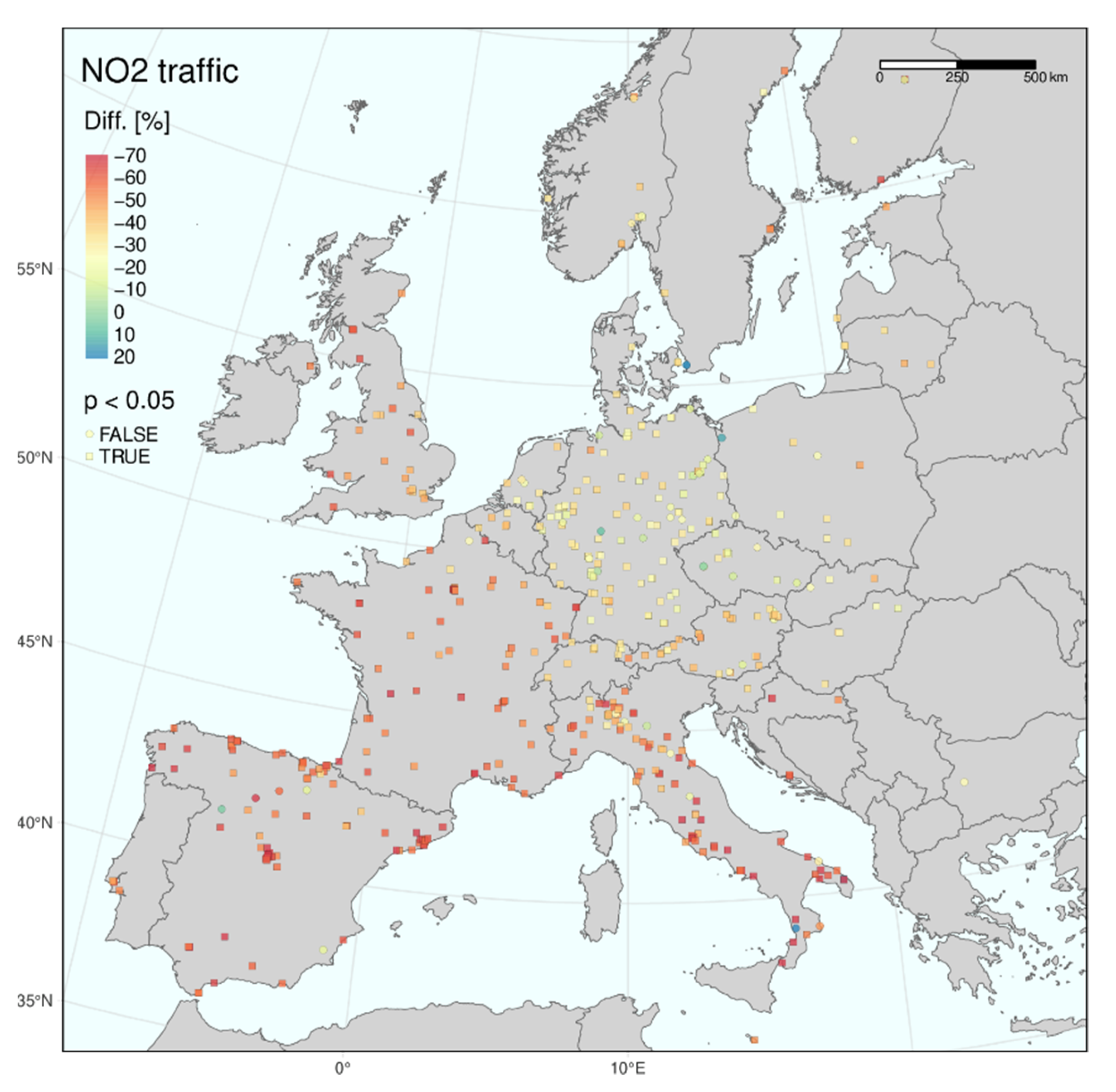
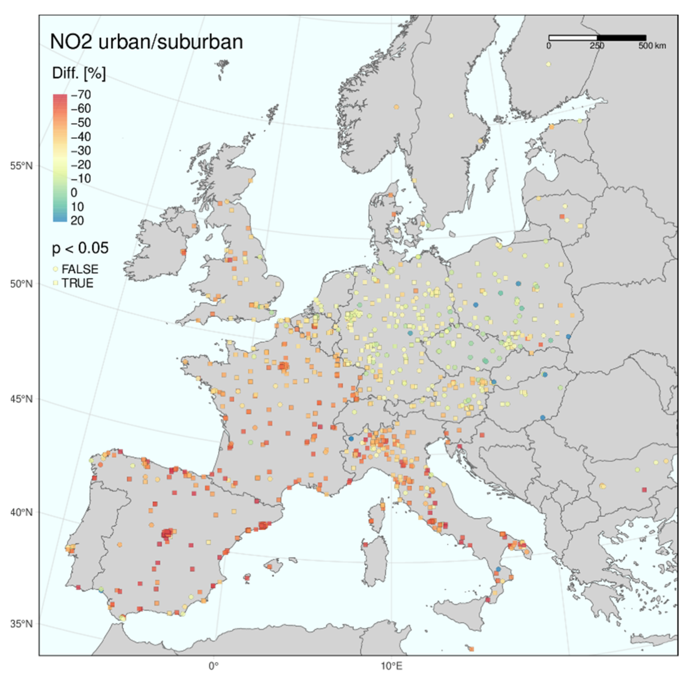
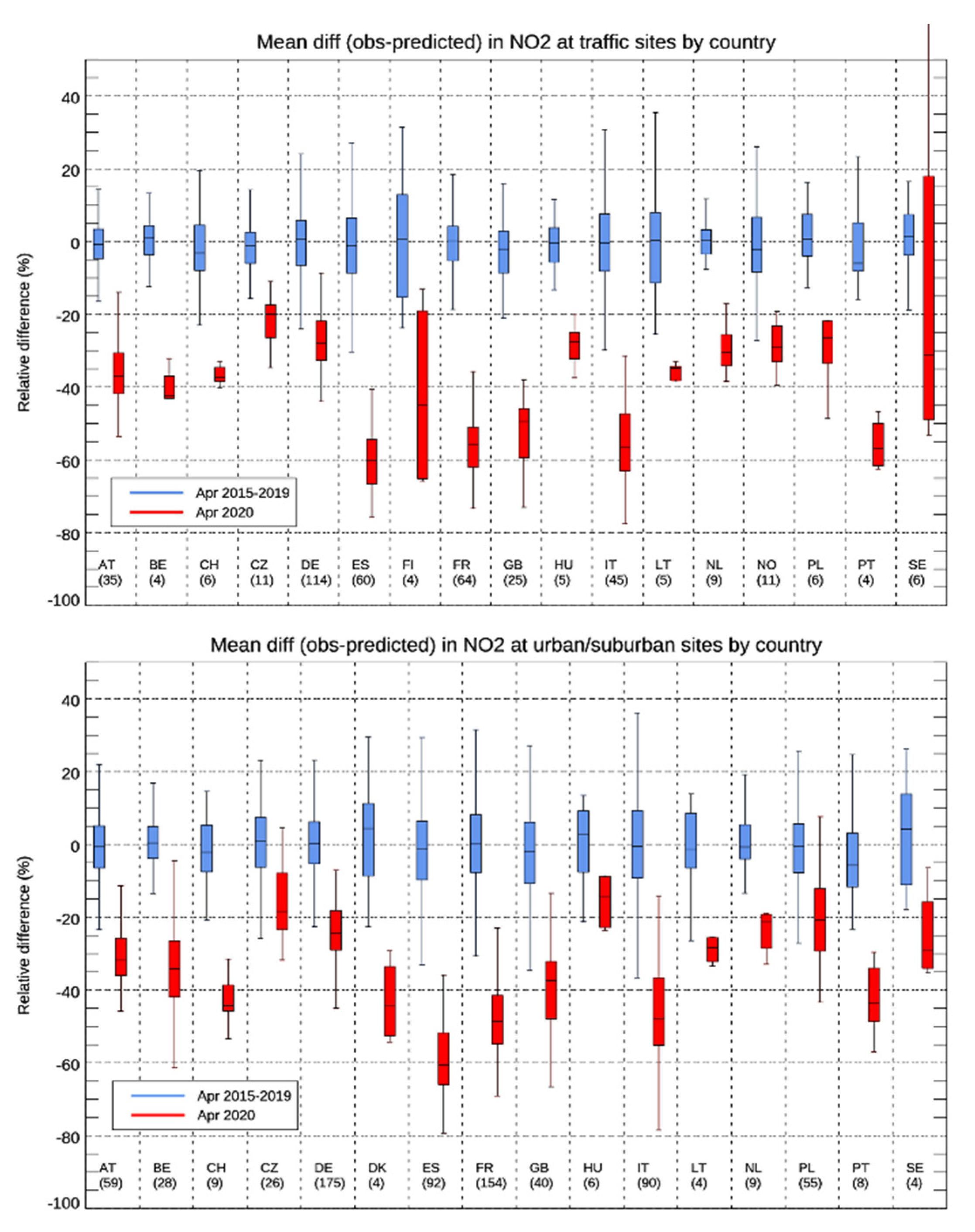
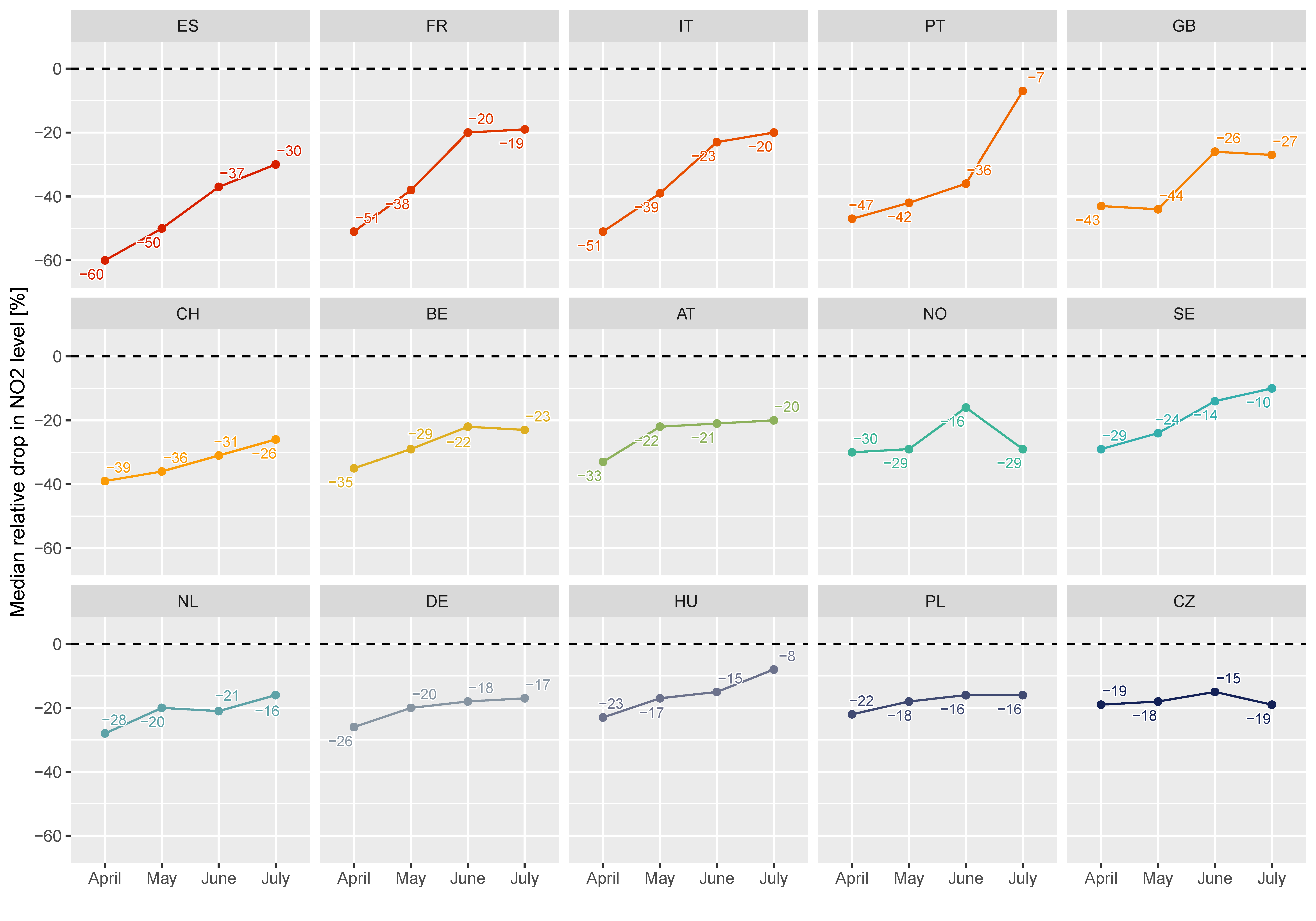
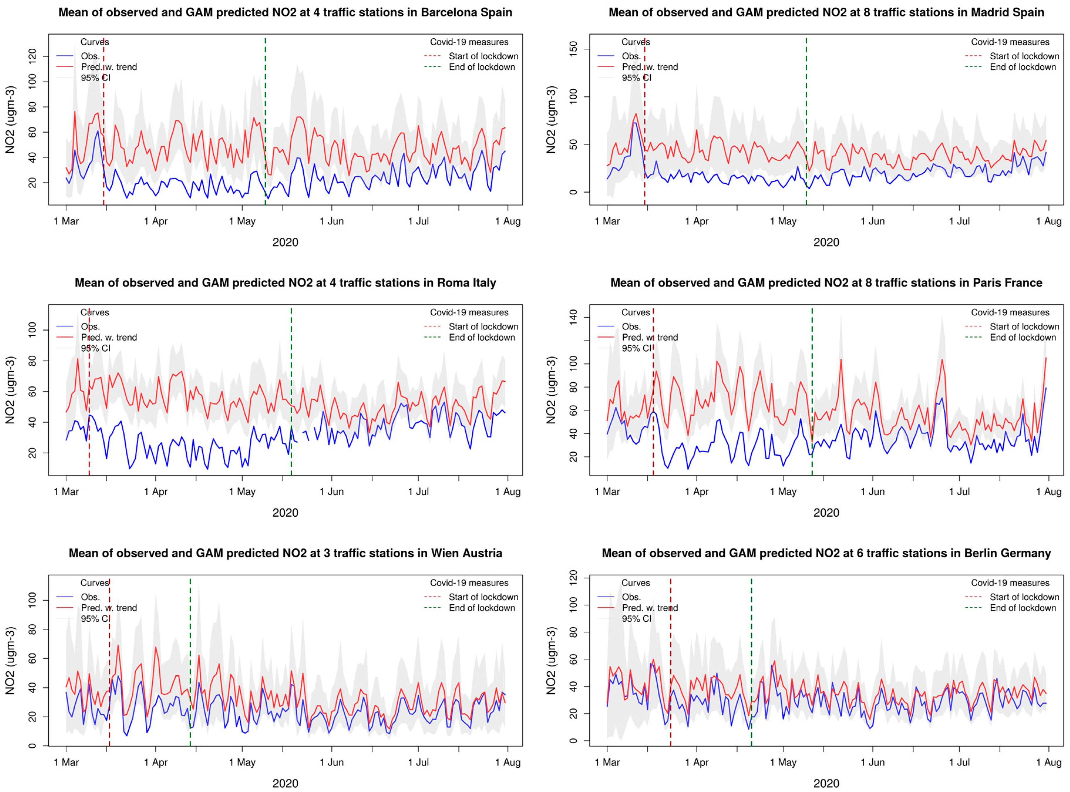
The results after aggregating all traffic sites (or urban/suburban sites) for individual countries show particularly good agreement between predicted and observed daily NO2 levels. This is likely an effect of station-wise peculiarities cancelling out. For the urban and suburban stations, we estimated the most substantial lockdown effect on NO2 in Spain with a 60% reduction as a country average, followed by Italy (51%), France (51%), Portugal (47%) and Great Britain (43%). The least impact was estimated for the eastern countries of Poland (22%) and Hungary (23%). Our results showed a gradual recovery during April–July for all countries. Still, even in July, the NO2 levels were 20% lower than expected in many countries, indicating that the effect of reduced emissions lasted long after the first lockdown restrictions had been lifted.
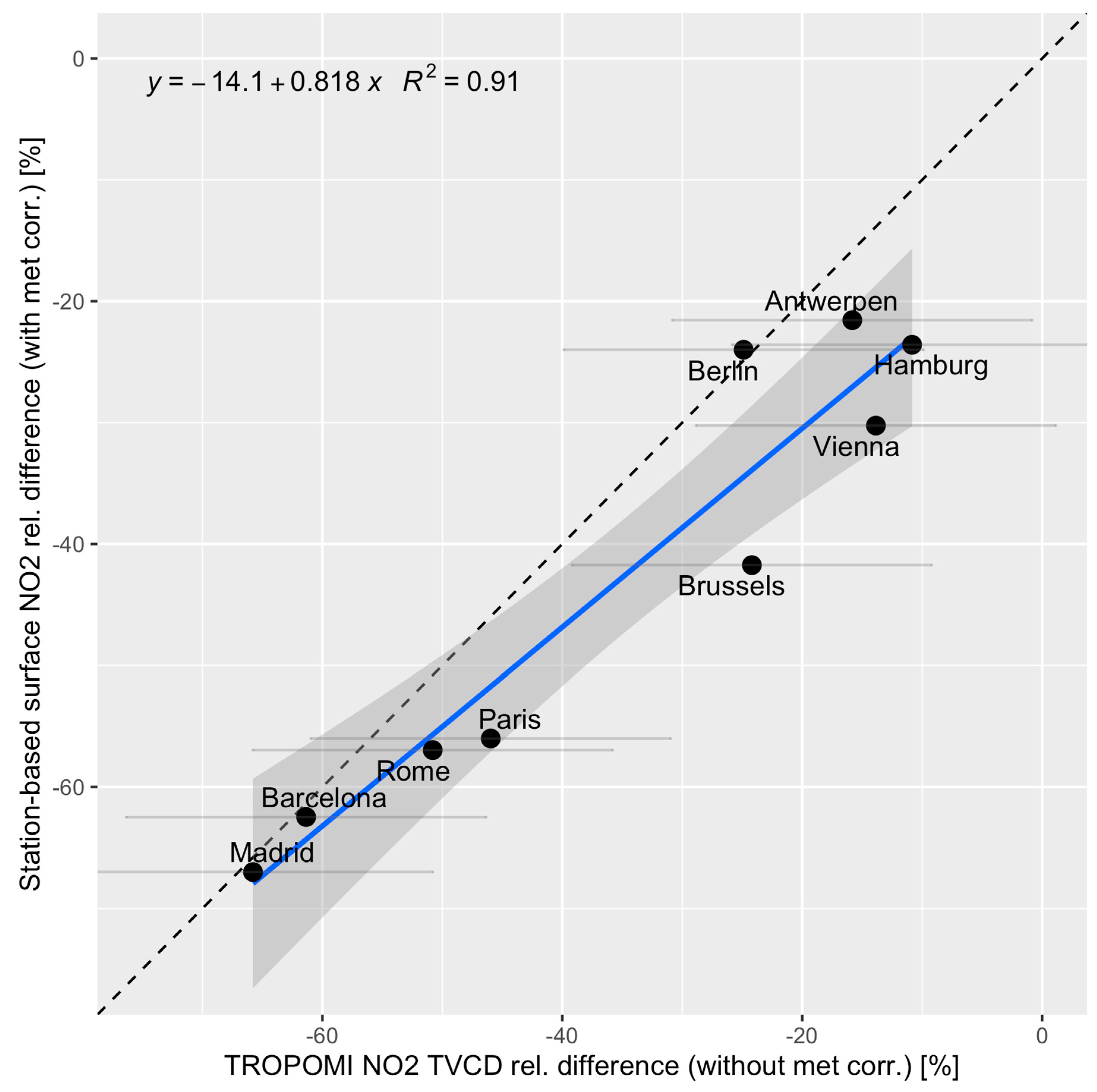
Aggregating the results for European cities also revealed large differences between the cities with Barcelona and Madrid on one end of the scale (mean reduction of around 60% in April) and Berlin, Hamburg and Vienna on the other end (20–30% reduction).
Whereas chemical transport models (CTMs) are state-of-the-art tools concerning assessment studies on a regional scale [26], they are less applicable for urban and roadside conditions. For these locations, statistical models such as the GAM could fill a gap assessing pollutants as documented in the present work.
The GAM has also been applied for PM10, PM2.5 and surface ozone [11,22,23] at rural, urban and suburban locations. The experience is that the GAM is indeed a valuable tool even for secondary pollutants at rural background sites, offering a low-cost model type that is complementary to resource-intensive CTMs. The GAM presented in this work will be applied to all of 2020, including the second wave and lockdown of the Covid-19 pandemic, as soon as the data are available.

Supplementary Materials

The following are available online at https://www.mdpi.com/2073-4433/12/2/131/s1, https://www.mdpi.com/2073-4433/12/2/131/s2 and https://www.mdpi.com/2073-4433/12/2/131/s3, Figure S1: time series plots of country averaged time series plots (observed and modelled) 2015–2020 based on traffic stations, Figure S2: time series plots of country averaged time series plots (observed and modelled) 2015–2020 based on urban and suburban background stations, Figure S3: time series plots of country averaged time series plots (observed and modelled) 2015–2020 based on rural stations.

Author Contributions

Conceptualisation, S.S., S.-E.W., C.G.; methodology, S.-E.W., S.S., C.G.; software, S.-E.W.; validation, S.S., S.-E.W., P.S.; formal analysis, S.S., S.-E.W., P.S.; resources, S.S.; data curation, S.S.; writing—original draft preparation, S.S.; writing—review and editing, S.S., S.-E.W., P.S., C.G.; visualisation, P.S., S.-E.W., S.S. All authors have read and agreed to the published version of the manuscript.

Funding

The authors are grateful for the financial support given by the European Environment Agency to the European Topic Centre on Air Pollution, Noise, Transport, and Industrial Pollution (ETC/ATNI) for this work, as well as the national contribution provided by the Norwegian Ministry of Climate and of Environment.

Institutional Review Board Statement

Not applicable.

Informed Consent Statement

Not applicable.

Data Availability Statement

The study did not report any data.

Acknowledgments

Sabine Eckhardt at NILU is acknowledged for extracting the meteorological data from ECMWF. The GAM model’s computations were performed on resources provided by UNINETT Sigma2—the National Infrastructure for High-Performance Computing and Data Storage in Norway.

Conflicts of Interest

The authors declare no conflict of interest.

References

  1. Sandford, A. Coronavirus: Half of Humanity on Lockdown in 90 Countries. Available online: https://www.euronews.com/2020/04/02/coronavirus-in-europe-spain-s-death-toll-hits-10-000-after-record-950-new-deaths-in-24-hou (accessed on 18 December 2020).
  2. Changes in Transport Behaviour during the Covid-19 Crisis—Analysis. Available online: https://www.iea.org/articles/changes-in-transport-behaviour-during-the-covid-19-crisis (accessed on 18 December 2020).
  3. Baldasano, J.M. COVID-19 Lockdown Effects on Air Quality by NO2 in the Cities of Barcelona and Madrid (Spain). Sci. Total Environ. 2020, 741, 140353. [Google Scholar] [CrossRef] [PubMed]
  4. Barré, J.; Petetin, H.; Colette, A.; Guevara, M.; Peuch, V.-H.; Rouil, L.; Engelen, R.; Inness, A.; Flemming, J.; Pérez García-Pando, C.; et al. Estimating Lockdown Induced European NO2 Changes. Atmos. Chem. Phys. Discuss. 2020. [Google Scholar] [CrossRef]
  5. Dacre, H.F.; Mortimer, A.H.; Neal, L.S. How Have Surface NO2 Concentrations Changed as a Result of the UK’s COVID-19 Travel Restrictions? Environ. Res. Lett. 2020, 15, 104089. [Google Scholar] [CrossRef]
  6. Grange, S.K.; Lee, J.D.; Drysdale, W.S.; Lewis, A.C.; Hueglin, C.; Emmenegger, L.; Carslaw, D.C. COVID-19 Lockdowns Highlight a Risk of Increasing Ozone Pollution in European Urban Areas. Atmos. Chem. Phys. Discuss. 2020. [Google Scholar] [CrossRef]
  7. Keller, C.A.; Evans, M.J.; Knowland, K.E.; Hasenkopf, C.A.; Modekurty, S.; Lucchesi, R.A.; Oda, T.; Franca, B.B.; Mandarino, F.C.; Díaz Suárez, M.V.; et al. Global Impact of COVID-19 Restrictions on the Surface Concentrations of Nitrogen Dioxide and Ozone. Atmos. Chem. Phys. Discuss. 2020, 1–32. [Google Scholar] [CrossRef]
  8. Menut, L.; Bessagnet, B.; Siour, G.; Mailler, S.; Pennel, R.; Cholakian, A. Impact of Lockdown Measures to Combat Covid-19 on Air Quality over Western Europe. Sci. Total Environ. 2020, 741, 140426. [Google Scholar] [CrossRef] [PubMed]
  9. Petetin, H.; Bowdalo, D.; Soret, A.; Guevara, M.; Jorba, O.; Serradell, K.; Perez Garcia-Pando, C. Meteorology-Normalized Impact of the COVID-19 Lockdown upon NO2 Pollution in Spain. Atmos. Chem. Phys. 2020, 20, 11119–11141. [Google Scholar] [CrossRef]
  10. Sicard, P.; De Marco, A.; Agathokleous, E.; Feng, Z.; Xu, X.; Paoletti, E.; Dieguez Rodriguez, J.J.; Calatayud, V. Ampli Fied Ozone Pollution in Cities during the COVID-19 Lockdown. Sci. Total Environ. 2020, 735, 139542. [Google Scholar] [CrossRef] [PubMed]
  11. European Environment Agency. Air Quality in Europe: 2020 Report; European Environmental Agency: Copenhagen, Denmark, 2020.
  12. Tobías, A.; Carnerero, C.; Reche, C.; Massagué, J.; Via, M.; Minguillón, M.C.; Alastuey, A.; Querol, X. Changes in Air Quality during the Lockdown in Barcelona (Spain) One Month into the SARS-CoV-2 Epidemic. Sci. Total Environ. 2020, 726, 138540. [Google Scholar] [CrossRef] [PubMed]
  13. Grivas, G.; Athanasopoulou, E.; Kakouri, A.; Bailey, J.; Liakakou, E.; Stavroulas, I.; Kalkavouras, P.; Bougiatioti, A.; Kaskaoutis, D.G.; Ramonet, M.; et al. Integrating in Situ Measurements and City Scale Modelling to Assess the COVID-19 Lockdown Effects on Emissions and Air Quality in Athens, Greece. Atmosphere 2020, 11, 1174. [Google Scholar] [CrossRef]
  14. Sharma, S.; Zhang, M.; Gao, J.; Zhang, H.; Kota, S.H. Effect of Restricted Emissions during COVID-19 on Air Quality in India. Sci. Total Environ. 2020, 728, 138878. [Google Scholar] [CrossRef] [PubMed]
  15. Dumka, U.C.; Kaskaoutis, D.G.; Verma, S.; Ningombam, S.S.; Kumar, S.; Ghosh, S. Silver Linings in the Dark Clouds of COVID-19: Improvement of Air Quality over India and Delhi Metropolitan Area from Measurements and WRF-CHIMERE Model Simulations. Atmos. Pollut. Res. 2020. [Google Scholar] [CrossRef]
  16. Li, L.; Li, Q.; Huang, L.; Wang, Q.; Zhu, A.; Xu, J.; Liu, Z.; Li, H.; Shi, L.; Li, R.; et al. Air Quality Changes during the COVID-19 Lockdown over the Yangtze River Delta Region: An Insight into the Impact of Human Activity Pattern Changes on Air Pollution Variation. Sci. Total Environ. 2020, 732, 139282. [Google Scholar] [CrossRef] [PubMed]
  17. Wang, Z.; Uno, I.; Yumimoto, K.; Itahashi, S.; Chen, X.; Yang, W.; Wang, Z. Impacts of COVID-19 Lockdown, Spring Festival and Meteorology on the NO2 Variations in Early 2020 over China Based on in-Situ Observations, Satellite Retrievals and Model Simulations. Atmos. Environ. 2021, 244, 117972. [Google Scholar] [CrossRef] [PubMed]
  18. Ordonez, C.; Garrido-Perez, J.M.; Garcia-Herrera, R. Early Spring Near-Surface Ozone in Europe during the COVID-19 Shutdown: Meteorological Effects Outweigh Emission Changes. Sci. Total Environ. 2020, 747, 141322. [Google Scholar] [CrossRef] [PubMed]
  19. Hastie, T.J.; Tibshirani, R.J. Generalized Additive Models; CRC Press: Boca Raton, FL, USA, 1990; Volume 43, ISBN 978-0-412-34390-2. [Google Scholar]
  20. Wood, S.N. Generalized Additive Models: An Introduction with R; Chapman and Hall/CRC: London, UK, 2017; ISBN 978-1-315-37027-9. [Google Scholar]
  21. Thampi, A. Interpretable AI. Available online: https://www.manning.com/books/interpretable-ai (accessed on 18 December 2020).
  22. Solberg, S.; Walker, S.-E.; Schneider, P.; Guerreiro, C.; Colette, A. ETC/ACM Technical Paper 2017/15; European Environmental Agency: Copenhagen, Denmark, 2018; p. 62.
  23. Solberg, S.; Walker, S.-E.; Guerreiro, C.; Colette, A. ETC/ATNI Report 14/2019: Statistical Modelling for Long-Term Trends of Pollutants. Use of a GAM Model for the Assessment of Measurements of O3, NO2 and PM; European Environmental Agency: Copenhagen, Denmark, 2020.
  24. Camalier, L.; Cox, W.; Dolwick, P. The Effects of Meteorology on Ozone in Urban Areas and Their Use in Assessing Ozone Trends. Atmos. Environ. 2007, 41, 7127–7137. [Google Scholar] [CrossRef]
  25. Dee, D.P.; Uppala, S.M.; Simmons, A.J.; Berrisford, P.; Poli, P.; Kobayashi, S.; Andrae, U.; Balmaseda, M.A.; Balsamo, G.; Bauer, P.; et al. The ERA-Interim Reanalysis: Configuration and Performance of the Data Assimilation System. Q. J. R. Meteorol. Soc. 2011, 137, 553–597. [Google Scholar] [CrossRef]
  26. Bessagnet, B.; Pirovano, G.; Mircea, M.; Cuvelier, C.; Aulinger, A.; Calori, G.; Ciarelli, G.; Manders, A.; Stern, R.; Tsyro, S.; et al. Presentation of the EURODELTA III Intercomparison Exercise—Evaluation of the Chemistry Transport Models’ Performance on Criteria Pollutants and Joint Analysis with Meteorology. Atmos. Chem. Phys. 2016, 16, 12667–12701. [Google Scholar] [CrossRef] [Green Version]
Figure 1. Distribution of r values for the generalised additive model (GAM) performance vs. observed daily mean concentrations at different station types for March–July 2015–2019. Stations with a value of r < 0.65 (threshold marked with a horizontal black line) were not used further in the analyses.
Atmosphere 12 00131 g001
Figure 2. Linear correlation coefficients (Pearson r) and normalised mean gross error (NMGE) for the GAM predicted vs. observed daily mean values of NO2 during March–July 2015–2019. Squares = traffic sites, diamonds = urban/suburban sites and circles = rural background sites. These maps show all stations before screening for r ≥ 0.65.
Atmosphere 12 00131 g002
Figure 3. The lockdown impact in April 2020 is given by the difference between the measured and predicted mean NO2 concentration for traffic sites. Stations with a statistically significant change (p < 0.05) are shown as squares, other with circles.
Atmosphere 12 00131 g003
Figure 4. Same as Figure 3 for urban/suburban sites.
Atmosphere 12 00131 g004
Figure 5. Same as Figure 3 for rural sites.
Atmosphere 12 00131 g005
Figure 6. The country-wise differences between measured and expected mean NO2 concentration in April 2020 for traffic sites (upper panel) and urban/suburban sites (lower panel). The numbers in brackets give the number of stations. Only countries with at least four stations in the given category were included in the figure. The centreline shows the median value while the boxes span from the 25- to 75-quantile and the whiskers from the 9- to the 91-quantile.
Atmosphere 12 00131 g006
Figure 7. The median relative drop in NO2 concentration at all urban and suburban sites is given by the difference between the GAM predicted and observed level in April–July 2020. Only countries with at least ten sites are shown.
Atmosphere 12 00131 g007
Figure 8. Daily mean NO2 levels as observed (blue) and predicted (red) by the GAM for 60 traffic stations in Spain during March–July 2015–2020. The start and end of the lockdown in 2020 are indicated in the plot. Grey shading indicates the 95 percent uncertainty in the prediction interval for each day, as explained in Section 3.
Atmosphere 12 00131 g008
Figure 9. Same as Figure 8 for traffic sites in the Czech Republic.
Atmosphere 12 00131 g009
Figure 10. Daily mean NO2 levels as observed (blue) and predicted (red) by the GAM for traffic stations in Barcelona, Madrid, Rome, Paris, Vienna and Berlin during March–July 2020. The start and end of the lockdown in 2020 are indicated in the plot. Grey shading indicates the 95 percent uncertainty in the prediction interval for each day, as explained in Section 2.
Atmosphere 12 00131 g010
Figure 11. Relative reduction (in percent) of the observed NO2 level for April 2020 compared to the business-as-usual scenario for all qualifying air quality monitoring stations in six selected cities (Barcelona, Madrid, Rome, Paris, Vienna and Berlin). Circles indicate traffic sites, squares indicate urban/suburban sites, and diamonds indicate rural sites. Note that the colour scale range varies between the panels to highlight the spatial patterns within a city better. In addition, note that in these maps, all stations within each domain are shown, whereas Figure 10 only shows stations selected according to a predefined list provided by EEA. Background base map by ESRI (Environmental Systems Research Institute) and contributors.
Atmosphere 12 00131 g011
Figure 12. Comparison of the average tropospheric vertical column density (TVCD) of NO2 retrieved from the TROPOMI instrument on board of the Sentinel-5P platform for April 2019 (left panel) and April 2020 (right panel). Units are given in 1015 molecules per square centimetre. Basemap copyright OpenStreetMap contributors and map tiles by Stamen Design, under CC BY 3.0.
Atmosphere 12 00131 g012
Figure 13. The relative difference in the tropospheric vertical NO2 column density as observed by the TROPOMI instrument on Sentinel-5P for April 2020 versus the GAM predicted relative reduction in surface NO2 concentration at traffic sites in various European cities. Gray horizontal lines represent the approximate uncertainties of the satellite estimates, including the effect of meteorological variability. The dashed black line indicates the 1:1 reference line.
Atmosphere 12 00131 g013
Table 1. List of input data used for the generalised additive model (GAM) calculations.
Explanatory Variable of the GAM Model
x1Daily temperature at 18 UT
x2Daily mean 10 m wind speed
x3Daily mean 10 m wind direction
x4Daily mean PBL height
x5Daily relative humidity at 18 UT 1
x6Weekday number
x7Day number in the season
x8Continuous-time in fraction of years (0.0 = 1 Jan at start of period). This is the trend term.
1 Relative humidity was not given in the ECMWF (European Center for Medium-Range Weather Forecast) data but was calculated based on the absolute humidity, temperature and pressure. UT = Universal Time. PBL = Planetary Boundary Layer.
Table 2. Statistical performance metrics for the GAM vs. daily mean concentrations of NO2 for March–July 2015–2019 for the three categories of stations. n = number of stations, r = linear correlation coefficient, NMGE = normalised mean gross error. The fraction of sites passing the screening (r > 0.65) is also given.
Before FilteringAccepted Sites (%)After Filtering
NrNMGE (%)NrNMGE (%)
Traffic sites5010.7320854240.7718
Urban and suburban background sites9650.7224817780.7722
Rural background sites3470.6030521810.7524
All sites18130.70247613830.7721
Publisher’s Note: MDPI stays neutral with regard to jurisdictional claims in published maps and institutional affiliations.

