
Seasonal Disparity in the Effect of Meteorological Conditions on Air Quality in China Based on Artificial Intelligence

Abstract
:1. Introduction
2. Literature Review
2.1. Meteorological Conditions and Air Quality
2.2. Research Technique
3. Methods
3.1. Sensitivity Analysis Based on Artificial Neural Network
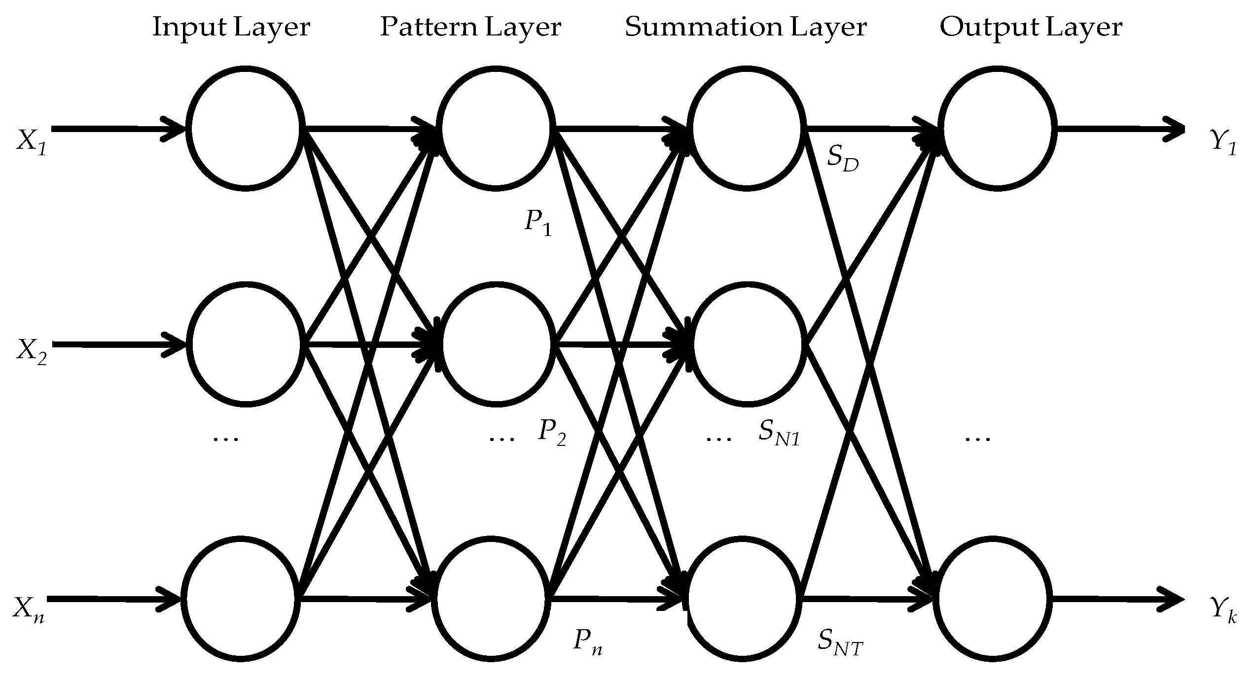
3.2. Generalized Regression Neural Network Model
- (1)
- Input layer
- (2)
- Pattern layer
- (3)
- Summation layer
- (4)
- Output layer
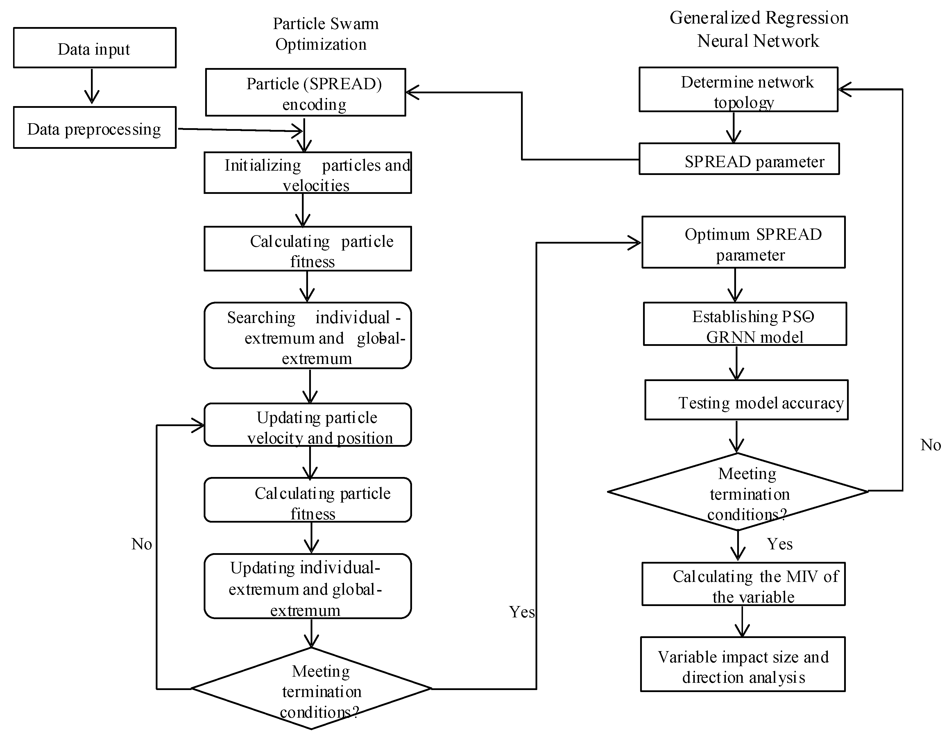
3.3. PSO-GRNN Model
4. Results
4.1. Statistic Analysis
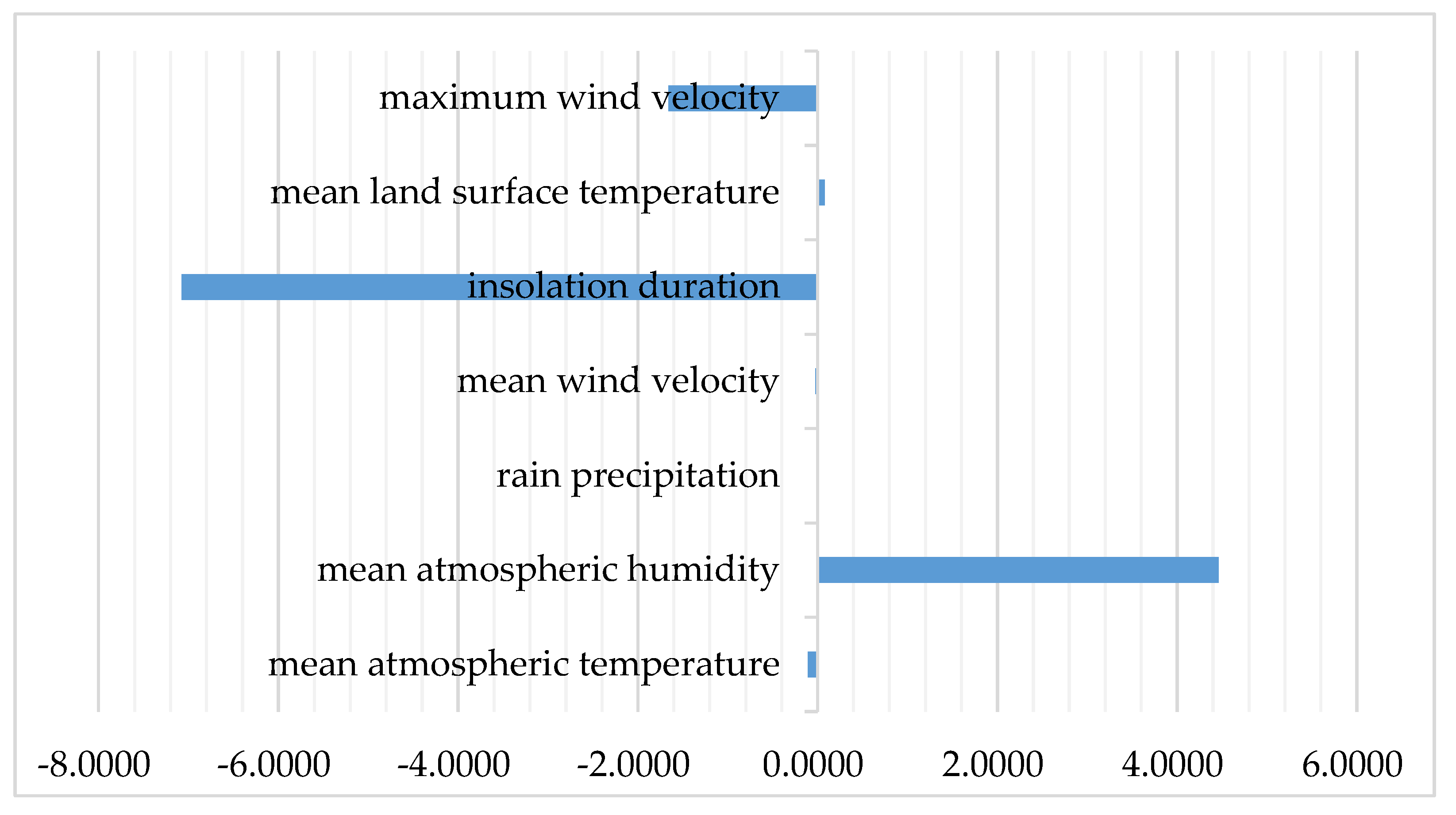
4.2. Impact Size Analysis
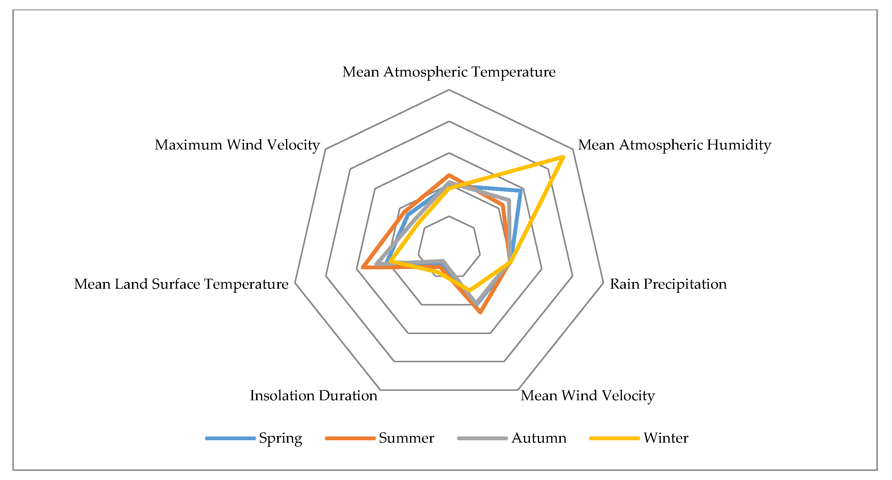
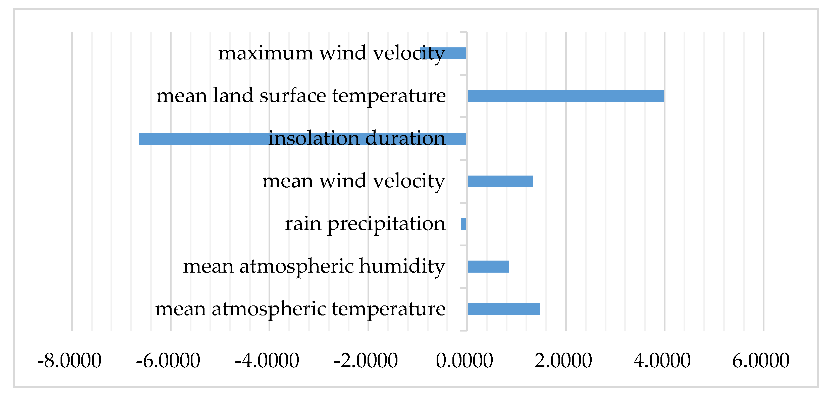
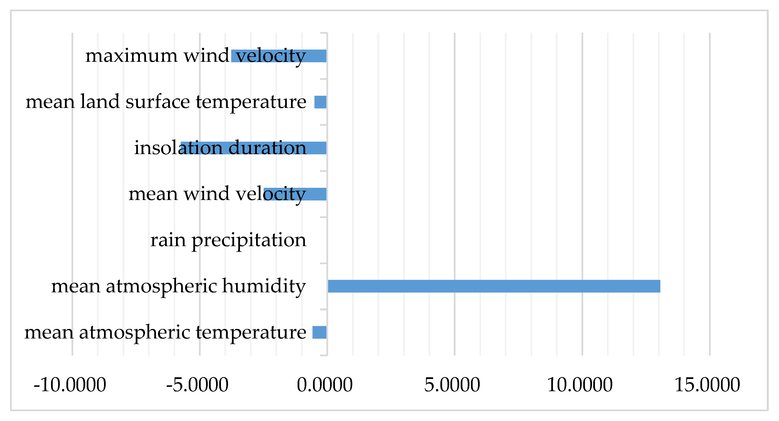
4.3. Seasonal Disparity Analysis
- (1)
- Spring Season
- (2)
- Summer Season
- (3)
- Autumn Season
- (4)
- Winter Season
5. Conclusions
Funding
Data Availability Statement
Conflicts of Interest
References
- Apte, J.S.; Brauer, M.; Cohen, A.J.; Ezzati, M.; Pope, C.A., III. Ambient PM2.5 Reduces global and regional life expectancy. Environ. Sci. Technol. Lett. 2018, 5, 546–551. [Google Scholar] [CrossRef] [Green Version]
- Cole-Hunter, T.; de Nazelle, A.; Donaire-Gonzalez, D.; Kubesch, N.; Carrasco-Turigas, G.; Matt, F.; Martinez, D. Estimated effects of air pollution and space-time-activity on cardiopulmonary outcomes in healthy adults: A repeated measures study. Environ. Int. 2018, 111, 247–259. [Google Scholar] [CrossRef] [PubMed]
- Cohen, A.J.; Brauer, M.; Burnett, R.; Anderson, H.R.; Frostad, J.; Estep, K.; Feigin, V. Estimates and 25-year trends of the global burden of disease attributable to ambient air pollution: An analysis of data from the Global Burden of Diseases Study 2015. Lancet 2017, 389, 1907–1918. [Google Scholar] [CrossRef] [Green Version]
- Chen, X.; Shao, S.; Tian, Z.; Xie, Z.; Yin, P. Impacts of air pollution and its spatial spillover effect on public health based on China’s big data sample. J. Clean. Prod. 2017, 142, 915–925. [Google Scholar] [CrossRef]
- Parker, J.D.; Mendola, P.; Woodruff, T.J. Preterm birth after the Utah Valley Steel Mill closure: A natural experiment. Epidemiology 2008, 19, 820–823. [Google Scholar] [CrossRef] [PubMed]
- Pope, C.A., III; Ezzati, M.; Dockery, D.W. Fine-particulate air pollution and life expectancy in the United States. N. Engl. J. Med. 2009, 360, 376–386. [Google Scholar] [CrossRef] [PubMed] [Green Version]
- Chai, F.; Gao, J.; Chen, Z.; Wang, S.; Zhang, Y.; Zhang, J. Spatial and temporal variation of particulate matter and gaseous pollutants in 26 cities in China. J. Environ. Sci. 2014, 26, 75–82. [Google Scholar] [CrossRef]
- Brauer, M.; Freedman, G.; Frostad, J.; Van Donkelaar, A.; Martin, R.V.; Dentener, F. Ambient air pollution exposure estimation for the global burden of disease 2013. Environ. Sci. Technol. 2015, 50, 79–88. [Google Scholar] [CrossRef]
- Yale Center for Environmental Law and Policy, International Earth Science Information Network (CIESIN), 2016 Environmental Performance Index. Available online: http://epi.yale.edu (accessed on 28 January 2016).
- Chen, Y.; Zhao, C.; Zhang, Q.; Deng, Z.; Huang, M.; Ma, X. Aircraft study of mountain chimney effect of Beijing, China. J. Geophys. Res. Atmos. 2009, 114, D08306. [Google Scholar] [CrossRef]
- Crippa, M.; Canonaco, F.; Slowik, J.G.; El Haddad, I.; De-Carlo, P.F.; Mohr, C. Primary and secondary organic aerosol origin by combined gas-particle phase source apportionment. Atmos. Chem. Phys. 2013, 13, 8411–8426. [Google Scholar] [CrossRef] [Green Version]
- Gao, Y.; Liu, X.; Zhao, C.; Zhang, M. Emission controls versus meteorological conditions in determining aerosol concentrations in Beijing during the 2008 Olympic Games. Atmos. Chem. Phys. 2011, 11, 12437–12451. [Google Scholar] [CrossRef] [Green Version]
- He, J.; Yu, Y.; Liu, N.; Zhao, S. Numerical model-based relationship between meteorological conditions and air quality and its implication for urban air quality management. Int. J. Environ. Pollut. 2013, 53, 265–286. [Google Scholar] [CrossRef]
- He, J.; Yu, Y.; Xie, Y.; Mao, H.; Wu, L.; Liu, N.; Zhao, S. Numerical model-based artificial neural network model and its application for quantifying impact factors of urban air quality. Water Air Soil Pollut. 2016, 227, 235. [Google Scholar] [CrossRef]
- Liu, T.; Gong, S.; Yu, M.; Zhao, Q.; Li, H.; He, J. Contributions of meteorology and emission to the 2015 winter severe haze pollution episodes in Northern China. Atmos. Chem. Phys. 2016, 1–17. [Google Scholar] [CrossRef] [Green Version]
- Pearce, J.L.; Beringer, J.; Nicholls, N.; Hyndman, R.J.; Uotila, P.; Tapper, N.J. Investigating the influence of synoptic-scale meteorology on air quality using self-organizing maps and generalized additive modelling. Atmos. Environ. 2011, 45, 128–136. [Google Scholar] [CrossRef]
- Wang, Y.; Ying, Q.; Hu, J.; Zhang, H. Spatial and temporal variations of six criteria air pollutants in 31 provincial capital cities in China during 2013–2014. Environ. Int. 2014, 73, 413–422. [Google Scholar] [CrossRef]
- Wu, Q.Z.; Wang, Z.F.; Gbaguidi, A.; Gao, C.; Li, L.N.; Wang, W. A numerical study of contributions to air pollution in Beijing during CAREBeijing-2006. Atmos. Chem. Phys. 2011, 11, 5997–6011. [Google Scholar] [CrossRef] [Green Version]
- Zhang, J.P.; Zhu, T.; Zhang, Q.H.; Li, C.C.; Shu, H.L.; Ying, Y. The impact of circulation patterns on regional transport pathways and air quality over Beijing and its surroundings. Atmos. Chem. Phys. 2012, 12, 5031–5053. [Google Scholar] [CrossRef] [Green Version]
- Zhang, L.; Liu, L.; Zhao, Y.; Gong, S.; Zhang, X.; Henze, D.K. Source attribution of particulate matter pollution over North China with the adjoint method. Environ. Res. Lett. 2015, 10, 084011. [Google Scholar] [CrossRef]
- He, J.; Gong, S.; Yu, Y.; Yu, L.; Wu, L.; Mao, H. Air pollution characteristics and their relation to meteorological conditions during 2014–2015 in major Chinese cities. Environ. Pollut. 2017, 223, 484–496. [Google Scholar] [CrossRef] [PubMed]
- Wang, Y.Q.; Zhang, X.Y.; Sun, J.Y.; Zhang, X.C.; Che, H.Z.; Li, Y. Spatial and temporal variations of the concentrations of PM 10, PM 2.5 and PM 1 in China. Atmos. Chem. Phys. 2015, 15, 13585–13598. [Google Scholar] [CrossRef] [Green Version]
- An, X.; Zuo, H.; Chen, L. Atmospheric environmental capacity of SO2 in winter over Lanzhou in China: A case study. Adv. Atmos. Sci. 2007, 24, 688–699. [Google Scholar] [CrossRef]
- Wen, W.; Cheng, S.; Chen, X.; Wang, G.; Li, S.; Wang, X.; Liu, X. Impact of emission control on PM 2.5 and the chemical composition change in Beijing-Tianjin-Hebei during the APEC summit 2014. Environ. Sci. Pollut. Res. 2016, 23, 4509–4521. [Google Scholar] [CrossRef] [PubMed]
- Han, T.; Xu, W.; Chen, C.; Liu, X.; Wang, Q.; Li, J. Chemical apportionment of aerosol optical properties during the Asia-Pacific Economic Cooperation summit in Beijing, China. J. Geophys. Res. Atmos. 2015, 120, 12–281. [Google Scholar] [CrossRef]
- Zhang, W.; Zhu, T.; Yang, W.; Bai, Z.; Sun, Y.L.; Xu, Y. Airborne measurements of gas and particle pollutants during CAREBeijing-2008. Atmos. Chem. Phys. 2014, 14, 301–316. [Google Scholar] [CrossRef] [Green Version]
- Jo, W.K.; Park, J.H. Characteristics of roadside air pollution in Korean metropolitan city (Daegu) over last 5 to 6 years: Temporal variations, standard exceedances, and dependence on meteorological conditions. Chemosphere 2005, 59, 1557–1573. [Google Scholar] [CrossRef]
- Calkins, C.; Ge, C.; Wang, J.; Anderson, M.; Yang, K. Effects of meteorological conditions on sulfur dioxide air pollution in the North China Plain during winters of 2006–2015. Atmos. Environ. 2016, 147, 296–309. [Google Scholar] [CrossRef]
- Laña, I.; Del Ser, J.; Padró, A.; Vélez, M.; Casanova-Mateo, C. The role of local urban traffic and meteorological conditions in air pollution: A data-based case study in Madrid, Spain. Atmos. Environ. 2016, 145, 424–438. [Google Scholar] [CrossRef]
- Gualtieri, G.; Toscano, P.; Crisci, A.; Di Lonardo, S.; Tartaglia, M.; Vagnoli, C. Influence of road traffic, residential heating and meteorological conditions on PM10 concentrations during air pollution critical episodes. Environ. Sci. Pollut. Res. 2015, 22, 19027–19038. [Google Scholar] [CrossRef]
- Luo, W.; Fu, Z. Application of generalized regression neural network to the agricultural machinery demand forecasting. Appl. Mech. Mater. 2013, 278-280, 2177–2181. [Google Scholar] [CrossRef]
- Hu, R.; Wen, S.; Zeng, Z.; Huang, T. A short-term power load forecasting model based on the generalized regression neural network with decreasing step fruit fly optimization algorithm. Neurocomputing 2017, 221, 24–31. [Google Scholar] [CrossRef]
- Ladlani, I.; Houichi, L.; Djemili, L.; Heddam, S.; Belouz, K. Modeling daily reference evapotranspiration (ET 0) in the north of Algeria using generalized regression neural networks (GRNN) and radial basis function neural networks (RBFNN): A comparative study. Meteorol. Atmos. Phys. 2012, 118, 163–178. [Google Scholar] [CrossRef]
- Marchioni, A.; Magni, C.A. Investment decisions and sensitivity analysis: NPV-consistency of rates of return. Eur. J. Oper. Res. 2018, 268, 361–372. [Google Scholar] [CrossRef] [Green Version]
- Cao, M.S.; Pan, L.X.; Gao, Y.F.; Novák, D.; Ding, Z.C.; Lehký, D.; Li, X.L. Neural network ensemble-based parameter sensitivity analysis in civil engineering systems. Neural Comput. Appl. 2017, 28, 1583–1590. [Google Scholar] [CrossRef]
- Jiang, J.L.; Su, X.; Zhang, H.; Zhang, X.H.; Yuan, Y.J. A novel approach to active compounds identification based on support vector regression model and mean impact value. Chem. Biol. Drug Des. 2013, 81, 650–657. [Google Scholar] [CrossRef]
- Zhang, Y.; Na, S.; Niu, J.; Jiang, B. The influencing factors, regional difference and temporal variation of industrial technology innovation: Evidence with the FOA-GRNN model. Sustainability 2018, 10, 187. [Google Scholar] [CrossRef] [Green Version]
- Holland, J.H. Adaptation in Natural and Artificial Systems; MIT Press: Cambridge, MA, USA, 1992. [Google Scholar]
- An, J.; He, G.; Qin, F.; Li, R.; Huang, Z. A new framework of global sensitivity analysis for the chemical kinetic model using PSO-BPNN. Comput. Chem. Eng. 2018, 112, 154–164. [Google Scholar] [CrossRef]
- Eberhart, R.; Kennedy, J. Particle swarm optimization. In Proceedings of the IEEE International Conference on Neural Networks, Perth, Western Australia, 27 November-1 December 1995; Volume 4, pp. 1942–1948. [Google Scholar]
- Chen, Z.; Cai, J.; Gao, B.; Xu, B.; Dai, S.; He, B.; Xie, X. Detecting the causality influence of individual meteorological factors on local PM2.5 concentration in the Jing-Jin-Ji region. Sci. Rep. 2017, 7, 40735. [Google Scholar] [CrossRef] [PubMed] [Green Version]


| Meteorological Factors | Spring | Summer | Autumn | Winter |
|---|---|---|---|---|
| Mean Atmospheric Temperature | 9.2347 | 25.0109 | 20.7122 | 1.1011 |
| Mean Atmospheric Humidity | 39.1625 | 54.1359 | 64.7609 | 50.1250 |
| Rain Precipitation | 0.3120 | 3.0413 | 2.4307 | 0.1095 |
| Mean Wind Velocity | 2.3933 | 2.2326 | 1.7606 | 1.9902 |
| Insolation Duration | 7.5810 | 7.5022 | 6.1688 | 5.6957 |
| Mean Land Surface Temperature | 10.8468 | 29.1016 | 22.4008 | −0.3644 |
| Maximum Wind Velocity | 9.1300 | 9.0997 | 7.1155 | 7.6190 |
| Mean Atmospheric Temperature | Mean Atmospheric Humidity | Rain Precipitation | Mean Wind Velocity | Insolation Duration | Mean Land Surface Temperature | Maximum Wind Velocity |
|---|---|---|---|---|---|---|
| 0.2870 | 5.1158 | −0.0806 | −0.3482 | −6.7892 | 1.3489 | −2.3340 |
| Meteorological Factors | Spring | Summer | Autumn | Winter |
|---|---|---|---|---|
| Mean Atmospheric Temperature | −0.1103 | 1.4782 | 0.3445 | −0.5761 |
| Mean Atmospheric Humidity | 4.4602 | 0.8380 | 2.0914 | 13.0540 |
| Rain Precipitation | −0.0164 | −0.1264 | −0.1708 | −0.0068 |
| Mean Wind Velocity | −0.0243 | 1.3392 | −0.2062 | −2.4918 |
| Insolation Duration | −7.0758 | −6.6482 | −7.6961 | −5.7453 |
| Mean Land Surface Temperature | 0.0787 | 3.9839 | 1.7917 | −0.4966 |
| Maximum Wind Velocity | −1.6598 | −0.9452 | −2.9479 | −3.7631 |
Publisher’s Note: MDPI stays neutral with regard to jurisdictional claims in published maps and institutional affiliations. |
© 2021 by the author. Licensee MDPI, Basel, Switzerland. This article is an open access article distributed under the terms and conditions of the Creative Commons Attribution (CC BY) license (https://creativecommons.org/licenses/by/4.0/).
Share and Cite
Zhang, Y. Seasonal Disparity in the Effect of Meteorological Conditions on Air Quality in China Based on Artificial Intelligence. Atmosphere 2021, 12, 1670. https://doi.org/10.3390/atmos12121670
Zhang Y. Seasonal Disparity in the Effect of Meteorological Conditions on Air Quality in China Based on Artificial Intelligence. Atmosphere. 2021; 12(12):1670. https://doi.org/10.3390/atmos12121670
Chicago/Turabian StyleZhang, Yongli. 2021. "Seasonal Disparity in the Effect of Meteorological Conditions on Air Quality in China Based on Artificial Intelligence" Atmosphere 12, no. 12: 1670. https://doi.org/10.3390/atmos12121670
APA StyleZhang, Y. (2021). Seasonal Disparity in the Effect of Meteorological Conditions on Air Quality in China Based on Artificial Intelligence. Atmosphere, 12(12), 1670. https://doi.org/10.3390/atmos12121670