Review on Parameterization Schemes of Visibility in Fog and Brief Discussion of Applications Performance

Abstract

Low visibility, associated with fog, severely affects land, marine, and air transportation. Visibility is an important indicator to identify different intensities of fog; therefore, improving the ability to forecast visibility in fog is an urgent need for social and economic development. Establishing a proper visibility parameterization scheme is crucial to improving the accuracy of fog forecast operation. Considering various visibility impact factors, including RH, N_d, D, LWC, the parameterization formula of visibility in fog, as well as their performance in meteorology operation, are reviewed. Moreover, the estimated ability of the visibility parameterization formulas combined with the numerical model is briefly described, and their advantages and shortcomings are pointed out.

1. Introduction

Visibility (VIS) is an indicator used to distinguish different intensities of fog based on the grade of fog forecast in the World Meteorological Organization (WMO) guide [1]. The decrease in atmospheric VIS, associated with the formation and development of fog weather, especially the explosive growth of fog, causes a severe impact on land, marine and, air transportation, and often cause traffic accidents such as car collisions in high-speed vehicles which can endanger people’s lives and property [2,3,4,5]. Fog is the most common and severe low–visibility weather occurrence, receiving much attention [6,7,8]. The number of articles including the word “fog” in Journals of American Meteorological Society alone was around 4700 until 2007 [9], with the addition of a further 4268 articles from 2007 to 2021 when searching them in the same way (https://journals.ametsoc.org, accessed on 1 December 2021), indicating that there is substantial interest in this subject.

Until now, our knowledge on the physics of fog remains limited, including the numerous physical processes influencing fog formation, development, and decay. Although the physical processes of fog, such as droplet microphysics [10,11,12,13,14,15,16], aerosol physics and chemistry [17,18,19,20,21], radiation [22,23], turbulence [24,25,26,27], large/small-scale dynamics [28,29,30,31], and surface conditions [32,33,34,35,36] have been widely investigated, the uncertainty of typical numerical forecast models estimating VIS is higher than 50% [37,38,39]. As to VIS estimation methods in meteorological operations, some forecasting methods provide pure mathematical statistical fitting without the explicit consideration of physical processes [40], such as climatological statistical methods [41], the rule-based statistical method [42,43], numerical model ensemble [39,44,45] and machine learning methods [43,46]. However, other methods, based on physical factors [47], e.g., extinction coefficient, relative humidity (RH) [48], liquid/ice water content (LWC) [49,50], droplet number concentration (N_d) and fog droplets size [4,14,51,52], which can establish a direct relationship to VIS, are widely adoptable in atmospheric numerical models [4,53,54,55,56,57,58,59,60,61]. Therefore, research on the relationship between the impact factors and VIS, and their application effects are summarized in the review.

In terms of the connection between microphysical parameters and VIS, many studies focused on the influence of the extinction coefficient, fog droplets size, N_d, and LWC on VIS. Among them, the effect of the extinction coefficient on visibility provides the basis of others. The Koschmieder’s law, as we know it, laid the foundation for visibility observation [1,62]. Other parameters related to the extinction coefficient were later studied, and LWC. George [63] pointed out that the fog droplet spectrum and LWC provide two crucial parameters that characterized the microphysical characteristics of fog and that an excellent inverse relationship exists between LWC and VIS. Eldridge [64] analyzed the influence of droplet growth on the formation and dissipation of fog, and proposed an empirical relationship between VIS and LWC. Through a comparison of the observation results with the conclusions of Houghton and Radford, Eldridge [65] pointed out that it was necessary to consider the effect of N_d on the relationship between VIS and LWC. There were inverse correlations between the microphysical parameters and VIS, and there were also correlations between the parameters themselves. Niu et al. [14] showed that when nucleation and condensation growth dominated, a pronounced positive correlation between N_d and LWC existed. When the D increased, and N_d was small, the LWC would also be smaller. Many other studies have discussed the relationship between VIS and the evolution of microphysical parameters [4,52,58]. The following sections will further categorize and explain the corresponding results and their applications in atmospheric numerical models. The characteristics of fog in a polluted environment are fairly remarkable; thus, parameterization schemes of VIS in fog that contains chemical composition or concentrations of aerosol are beyond the scope of this article.

There are many factors impacting VIS in fog, and only several common physical elements, including RH, extinction coefficient, LWC, N_d, and fog droplets size, are introduced in this review due to the length limit. The following sections will summarize corresponding parameterization schemes of VIS in fog and their applications in meteorological operations.

2. Relationships between VIS and Extinction Coefficient

As early as the 1920s, based on the interference effects of fog and haze on the horizontal visual range, the Koschmieder’s law was proposed [62]. The theory assumes that the atmosphere is uniform, the horizontal extinction coefficient (β_ext) of the atmosphere is constant, and the flat sky is used as the background black body target during the day. Then the brightness contrast threshold (C) between the target and the background changes with the distance (VIS), and the relationship is as follows:

$$C=\exp \left(-{\beta }_{ext}·VIS\right),$$

(1)

which can be transformed as

$$VIS=\frac{1}{{\beta }_{ext}}ln\frac{1}{C},$$

(2)

where ${\beta }_{ext}$ is measured in units of inverse kilometers, the constant C is a physical quantity related to the human eye, there are two values for the contrast threshold C, the value recommended by the International Civil Aviation Organization (ICAO) is 0.05, and the value recommended by WMO is 0.02. Therefore, as long as the atmospheric extinction coefficient is obtained, the VIS value can be obtained. The daytime-target visual range theory proposed by this law has been the basis of manual VIS observation during daytime for many years. The most significant contribution of the Koschmieder’s law is that it first links VIS to the atmospheric extinction coefficient, which has become the theoretical basis for studying atmospheric VIS. To this day, this law is still the basic principle of various optical VIS measuring instruments. Inverse proportionality between VIS and β_ext is only applicable under very minimal conditions: the atmosphere must be illuminated homogeneously, the extinction coefficient and the scattering function are not allowed to vary with space, the object should ideally be black and viewed against the horizon, and the eye of the observer must have a constant contrast threshold. Horvath et al. [66] proposed a general formula, taking the facts above into account. Through the proper selection of the VIS markers, it is possible to use the Koschmieder’s formula to calculate the extinction coefficient from observed visibilities with an error of less than about 10 percent. Using radiative transfer theory, Lee et al. [67] point out that the Koschmieder’s model is workable only in situations where a common-sized object can be viewed tens of kilometers away, but not applicable for viewable distances of hundreds of meters when the angular dimension of an object is significantly greater than the eye resolution of the human being. Lee et al.’s research advocates for the measurement and distribution of detectability in bad weather.

The scattering theory of particles, proposed by Mie [68], is the basis for calculating the extinction coefficient. Since the diameter of the particles is equivalent to the wavelength of the light, the forward-scattered light is stronger than the backward-scattered light, and the scattering intensity is much larger than that of Rayleigh scattering. The β_ext in Mie scattering theory is given as follows:

$${\beta }_{ext}=\frac{2}{x^2}{{\displaystyle \sum }}_{n=1}^{\infty }\left(2n+1\right)Re\left(a_n+b_n\right),$$

(3)

where a_n and b_n are functions related to the Bessel function and Hankel function, and x is the radius of the droplet. In 1971, according to Beer’s law, Koening [69] pointed out that brightness was a function of the microphysical characteristics of the fog, which is due to the dependence of the extinction coefficient on the concentration and radius of the fog droplets. That is, β_ext is related to the N_d, droplet radius, visible light wavelength, etc. Kunkel [70] pointed out that if the drop-size distribution is known, then β_ext can be readily determined from the following equation (Equation (4))

$${\beta }_{ext}=\pi {{\displaystyle \sum }}_{i=1}^N{Q}_{ext}{n}_i{r}_i{}^2,$$

(4)

where Q_ext is the extinction efficiency (normalized extinction cross-section), n is the N_d, and r is the droplet radius. Moreover, If the drop-size distribution is unknown, then an empirical formula must be used to relate the LWC to β_ext, and related content is discussed in detail in the next section.

The total extinction coefficient is a sum of components from clean air, aerosol, cloud, and precipitation. The extinction coefficient for aerosols contains a contribution from different aerosol species, such as sea salt, dust, black carbon, organic matter, sulfates, and so on [71]. The extinction coefficient of clean air is small and has little practical value, so it is taken to be equivalent to a VIS of 100 km (10⁵ m), which defines the maximum VIS that can be diagnosed [72], that is ${\beta }_{air}=\left(lne\right)/{10}^5$.

The parameterization scheme based on Equation (2) was generally adopted by subsequent numerical research, providing a feasible scheme for the numerical forecast of horizontal VIS [73,74,75]. This scheme strongly relies on β_ext. Koening’s research [69] shows that the scheme is determined by multiple factors, which will lead to certain errors in calculations and measurements. For example, Kunkel [70] compared the extinction coefficient β_c, calculated through the droplet spectral distribution and the actually observed β_m, showing that the calculated extinction coefficient β_c is larger than the observed β_m. The results of Vali et al. [76] also showed that there was a deviation between the calculated value of the extinction coefficient and the measured value. The correction method proposed by Kunkel [70] is as follows:

$${\beta }_m=2.156{\beta }_c^{0.717}$$

(5)

There is significant uncertainty in calculating the extinction coefficient β_c through the droplet spectrum distribution. Therefore, if the VIS is calculated by Equation (2), certain errors will inevitably occur.

In aviation applications, not only horizontal but also vertical VIS has a significant impact on aircraft take-off and landing. Stoelinga and Warner [77] believed that the maximum horizontal VIS for aviation applications was 10 km, which was smaller than the horizontal grid spacing set in the NWP (such as 36 km and 12 km). Therefore, it could be considered that the extinction coefficient has a fixed value, and Equation (2) could be used to calculate the horizontal VIS. However, this assumption was no longer valid when calculating the vertical VIS, because the vertical maximum height (2500 m) that aviation considered was significantly greater than the vertical grid spacing (50–500 m) in the model. The extinction coefficient, which was closely related to the atmospheric environment, varied greatly in different model levels. Therefore, the extinction coefficient should be a function of height z, and the expression must be integrated layer by layer in an upward direction (replacing x with z) to determine the ceiling z_clg [77]:

$$-\ln \left(0.02\right)={{\displaystyle \int }}_0^{z_{clg}}\beta \left(z\right)dz,$$

(6)

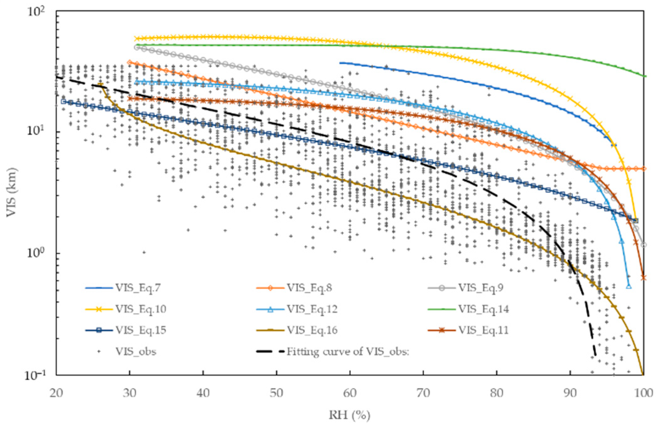
3. Relationships between VIS and RH

Fog is a weather phenomenon with a horizontal VIS of less than 1 km due to water vapor near the ground condensing into tiny water droplets or ice crystals and becoming suspended in the air [1]. Air saturation is the prerequisite for the appearance of fog weather in a clean atmosphere. Since human activities produce many aerosols which absorb moisture and also contribute to poor VIS, pollution fog affected by industrialization often occurs when the atmosphere does not reach saturation conditions [78,79]. VIS decaying in the unsaturated atmosphere is closely related to increasing RH. Therefore, summarizing the empirical relationship between VIS and RH, which can be used in the atmospheric numerical models to output the final VIS value, has certain practicability. In 1976, Hanel [80] proposed an empirical formula between VIS and RH, and the empirical equation is as follows:

$$VIS=67.7{\left(1-RH\right)}^{0.67},$$

(7)

Equation (7) is valid under the condition of 58% < RH < 97%. Due to only a single factor being involved in the empirical formula, the simple, clear formula can reflect the changing trend of unsaturated atmospheric VIS well and can guide for forecasting. Based on Hanel’s work, Smirnova et al. [81] further improved the VIS-RH empirical formula, following Equation (8),

$$VI{S}_{RUC}=60\exp \left(-2.5\left(RH-15\right)/80\right),$$

(8)

the condition of Equation (8) is 30% < RH ≤ 100%. The parameterization scheme is applied using the Rapid Update Cycle (RUC) model of the National Environmental Forecast Center of the United States. Based on the Fog Remote Sensing And Modeling (FRAM) at Pearson Airport, and the Alliance Icing Research Study (AIRS 2) at Mirabell Airport in Canada, Gultepe et al. [82] pointed out that Smirnova’s scheme used in the RUC is not applicable in Canada, and further identified a significant issue in that when the RH was close to 100%, the calculated VIS using the Smirnova’s scheme was approximately twice of the observed value. Based on the ground observation data of two airports, the more suitable VIS parameterization schemes for forecasting local VIS are provided in Equation (9),

$$VI{S}_{FRAM}=-41.5\ln \left(RH\right)+192.3,$$

(9)

and Equation (10)

$$VI{S}_{AIRS}=-0.0177R{H}^2+1.462RH+30.8.$$

(10)

The newly proposed scheme, applied in the numerical model, showed better application performance and the proved to be more suitable for local VIS forecasting. However, the VIS-RH schemes proposed by Gultepe [82] are not applicable in other regions. Cao et al. [83] studied the VIS parameterization scheme in the fog model of Dalian, China, and also found that under high humidity conditions, the calculation value of Smirnova’s scheme was significantly greater than the actual observation value. For example, when RH = 100%, VIS_RUC = 4.2 km; moreover, approximate 95.3% of the measured VIS ≤ 1 km. If this scheme is used to calculate visibility, when RH is high, the calculated result will be significantly larger than the observed value. A more suitable VIS-RH relationship was proposed based on the Dalian ground observation data. The newly built scheme [83] had greatly enhanced the local low VIS forecasting ability and is represented in Equation (11).

$$VIS=-0.00003272R{H}^3+0.00238R{H}^2-0.1165RH+21.2$$

(11)

It can be seen from Equation (11) that when RH = 100%, VIS = 0.63 km, when RH = 95%, VIS = 3.56 km, and when RH < 80%, VIS > 10 km. The revised VIS-RH parameterization scheme has greatly improved the ability to predict local low visibility compared to RH-VIS formula developed by Smirnova [81] and Gultepe [82].

In 2009, Gultepe et al. [84] further analyzed the relationship between VIS and RH, and pointed out that the VIS-RH relationship, based only on observational data fittings cannot be well used for VIS calculations, because for the same RH, the corresponding VIS value varied greatly. Therefore, Gultepe et al. [84] proposed a probability method, that is, a method in which all VIS values for the same RH are sorted by value, and the top 5%, 50%, and 95% of the data sets are used to fit, so as to meet different needs, respectively. For example, due to the concern of extremely poor VIS at an airport, it is more meaningful to obtain a possible minimum VIS value than to know the most likely VIS value. Therefore, the forecast scheme with 5% of the data is more practical, meaning that 95% of the data points have a higher VIS value. Gultepe et al. suggested the replacement of the deterministic forecast with the probability method, and the established parameterization scheme was found to be more suitable for the actual local meteorology operation. Lin et al. [85] performed the local application of the above probability method in Sichuan Province. The prediction effect of the mesoscale Weather Research and Forecasting Model (WRF) on the RH was evaluated, and the VIS-RH parameterization scheme by the measured VIS and RH data from Chengdu Shuangliu airport was obtained. The test results showed that the VIS values of the dense fog calculated by the VIS-RH parameterization scheme, which accounted for 5% of the data, were the most accurate, that is, the fitting curve with a probability of 5% was the closest to the low VIS both in trend and magnitude.

Fog is sensitive to meteorological factors. Even under the same weather condition, fog formation is still a probability event. The method proposed by Gultepe et al. [84]. can provide the probability of low VIS under the same RH condition, but the results are limited by the sampling. By the LEPS (Local Ensemble Prediction System), based on ensemble forecast, which can directly output the probability of LVP (Low VIS Procedure) events, Roquelaure et al. [86] carried out low VIS prediction assessment of Paris Charles de Gaulle Airport. The category of LVP can be obtained according to the established comparison table of event probability and categories. The results show that the system can reduce false alarms by 50–60%.

Results from some studies investigating the VIS-RH relationship are listed in

Table 1. The related VIS-RH parameterization schemes.

Equation No	Relationship	Conditions	Reference
(7)	$VIS=67.7{\left(1-RH\right)}^{0.67}$	RH in decimal form For 58% < RH < 97%	Hanel [80]
(8)	$VI{S}_{RUC}=60\exp \left[-2.5\left(RH-15\right)/80\right]$	For 30% ≤ RH ≤ 100% Set to 5 km at RH ≥ 95%	Smirnova et al. [81]
(9)	$VI{S}_{FRAM-C}=-41.5\ln \left(RH\right)+192.30$	For RH > 30%	Gultepe et al. [82]
(10)	$VI{S}_{AIRS}=-0.0177R{H}^2+1.46RH+30.80$	For RH > 30%	Gultepe et al. [82]
(11)	$VI{S}_{MX11}=-0.00003272R{H}^3+0.00238R{H}^2-0.1165RH+21.2$	For 30% ≤ RH ≤ 100%	Cao et al. [83]
(12)	$VI{S}_{FRAM-L\left(5\%\right)}=-0.000114R{H}^{2.7}+27.45$	For RH > 30%	Gultepe et al. [84]
(13)	$VI{S}_{FRAM-L\left(50\%\right)}=-5.19\times {10}^{-10}R{H}^{5.44}+40.10$	For RH > 30%	Gultepe et al. [84]
(14)	$VI{S}_{FRAM-L\left(95\%\right)}=-9.68\times {10}^{-14}R{H}^{7.19}+52.20$	For RH > 30%	Gultepe et al. [84]
(15)	$VI{S}_{Fit}=63.19-13.04\ln \left(RH+11.31\right)$	For 20% < RH < 100%	Lin et al. [85]
(16)	$VI{S}_{Fit-5\%}=21.38-4.938\ast \ln \left(RH-24.53\right)$	For 25% < RH < 100%	Lin et al. [85]

. Using VIS and RH observation data from the automatic weather station(AWS) from 2016 to 2017 in Tianjin urban meteorological observation (Tianjin), a localized VIS-RH scheme based on the probability method of 5%, proposed by Gultepe et al. [84], was made. The results show that T5, T10, T9, and the localized fitting curve can represent low VIS under the condition of high RH, but T5 overestimates VIS for all RH, and T10 also overestimates VIS under the condition of RH > 95% and RH < 40%. Comparatively speaking, the localized fitting curve can denote a better VIS-RH relationship (Figure 1).

Even though the VIS-RH schemes vary in different regions and have obvious regional characteristics, the VIS-RH relationship has been widely used in various models, including Numerical Weather Prediction (NWP) and fog models [87,88,89]. The RH value is easily obtained through the atmospheric numerical model, and it is also a direct observational element, which is convenient for VIS-RH verification. For the same RH value, the calculated VIS values vary in a wide range. Moreover, there are significant differences between VIS parameterization schemes, and the calculation accuracy cannot meet the needs of refined forecasting services. At present, most NWP and fog models no longer use VIS-RH schemes separately.

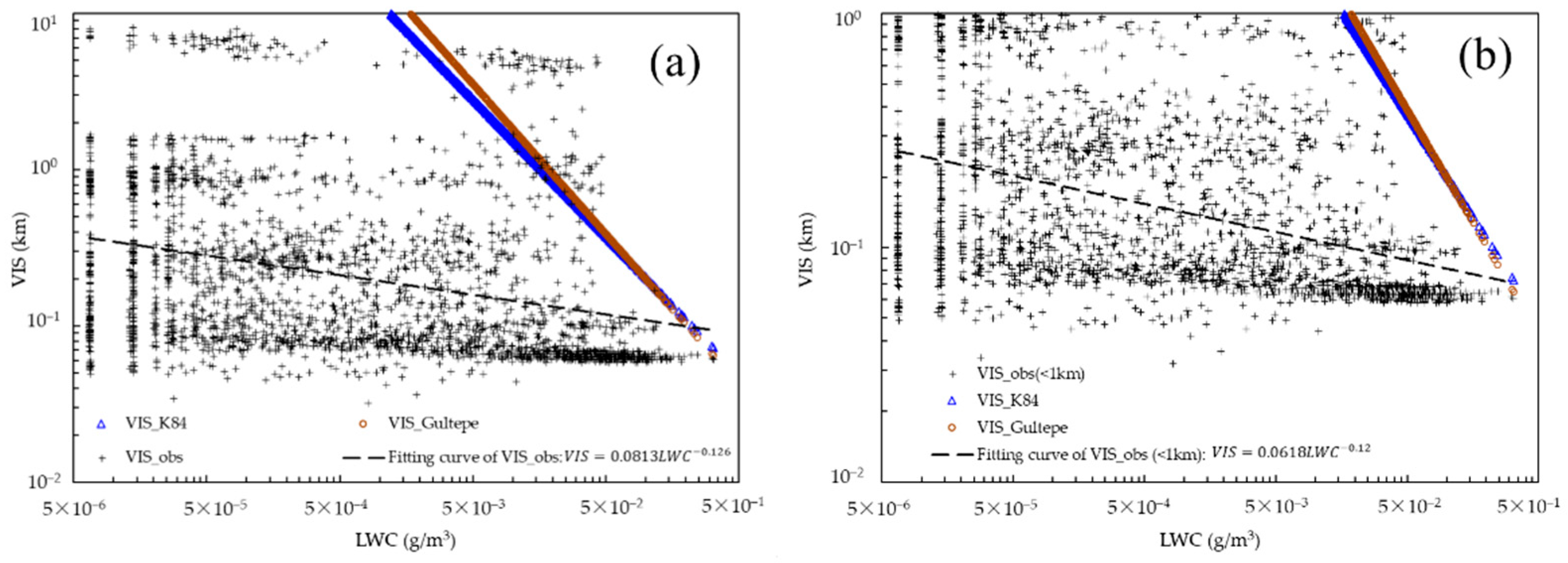
4. Relationships between VIS and LWC

The VIS-LWC scheme, based on the Koschmieder’s law [62], is relatively common in VIS parameterization schemes. The scheme calculates the VIS using LWC, and Equation (17) is as follows:

$$VIS=-\frac{\ln \left(0.02\right)}{{\beta }_{ext}}=a\ast LW{C}^b,$$

(17)

where LWC is provided in g/m³. A large number of studies have shown that the relationship between β_ext and LWC satisfies the power–function relationship mentioned above. The values of empirical coefficients a and b from various regions vary greatly. The size distributions of droplets are affected by many factors such as the observation range of droplet size, experiment design, air particulates, and fog types. For example, in 1966 and 1971, Eldridge [65,90] conducted a comparative analysis of different droplet size ranges through experiments, and the obtained empirical values of a and b varied across a broad range. When the droplet size is between 0.6 and 16 μm, $\beta =163LW{C}^{0.65}$, and when the upper limit of the droplet size range increases, $\beta =91LW{C}^{0.65}$. In 1976, Tomasi and Tampieri [91] obtained empirical values of a and b for different types of fog. Under the warm and humid fog conditions $\beta =65LW{C}^{2/3}$ was obtained, while $\beta =115LW{C}^{2/3}$ was obtained under cold fog conditions. In the existing research, the empirical coefficient ranges from 65 to 178, and b ranges from 0.63 to 0.96 [58]. It can be seen that the performance of the VIS-LWC parameter scheme is analogous to that of the VIS-RH scheme, which is also affected by many other factors and has a strong regional character.

At present, the most commonly used VIS-LWC program is the K84 program. In 1984, Kunkel [70] found that the correlation coefficient between the extinction coefficient and LWC reached 95% in the observational study of advection fog. Compared with the research results of other studies [90,91,92], there is a higher correlation between the two parameters. Kunkel [70] proposed the formula for calculating the extinction coefficient with the LWC in the fog, which is given as follows

$$\beta =144.7LW{C}^{0.88}.$$

(18)

Substituting this formula into the Koschmieder’s law (Equation (2)), the K84 scheme is obtained as follows:

$$VIS=0.027LW{C}^{-0.88}.$$

(19)

Some models work with LWC, and the K84 scheme provides a convenient solution for relating LWC to VIS. So, the K84 scheme is widely used in numerical models to calculate the values of VIS [54,73,74,75,89,93,94]. However, the K84 scheme was still improved as following Equation (20) by Gultepe [58] using Radiation and Aerosol Cloud Experiment (RACE) observation in 1995 in the eastern Canada area.

$$VIS=0.0219LW{C}^{-0.9603}$$

(20)

The LWC, N_d from the fog droplet spectral observation and VIS from AWS during 2016–2017 in TianJin [16] were used to validate VIS parameter formulas from literatures and to fit the local formula. The observation VIS and LWC ranged from 0 to 8.2 km and 0 to 0.25 g/m³, respectively. The VIS_K84 [70] and VIS_Gultepe schemes [58] were verified in Figure 2 with a logarithmic plot. It should be pointed out that only data for VIS that were less than 1 km were adopted in Figure 2a, while the full range of observation data was adopted in Figure 2b.

The VIS_K84 and VIS_Gultepe schemes simulation show a sharply decreasing VIS trend with LWC increasing. However, both of them are obviously larger than observation VIS especially for VIS less than 1 km in fog events. Deviations between simulated and observed VIS shows that something need to do to improve current VIS-LWC relationships. The local relationship of VIS and LWC was fitted as$VIS=0.0618LW{C}^{-0.126} \mathrm{and}VIS=0.0813LW{C}^{-0.126}$when using the VIS data less than 1 km and the full range of data, respectively. The local VIS-LWC shows a flatter decline than the VIS_K84 and VIS_Gultepe schemes, which are denoted by the black dashed line. It is due to a larger number of VIS observations being located at numerical intervals of less than 1 km. Evidently, the local fitting formula does not have the ability to express a VIS of larger than 1 km when LWC exists. So, no satisfactory corresponding relationship has been found between VIS and LWC as of yet.

Most of the visibility values simulated by the visibility parameterization schemes are greater than the observed values, as Figure 2 shows. Some widely used VIS parameterization schemes are conducted where air pollution is commonly not serious. When applied to fog forecast/simulation in the polluted environments, these schemes may overestimate VIS and underestimate fog intensity due to the absence of aerosol extinction [95,96].

So far, the three parameterization schemes of VIS-RH, VIS-β, and VIS-LWC, which correspond to the three key elements of RH, β and LWC respectively, have been discussed in this study. There are certain correlations that exist between the three elements, and research on the relationship between β and LWC has been introduced in this section. Some studies demonstrate a negative correlation between RH and LWC. For example, Gonser et al. [97] first revealed the inverse relationship between RH and LWC in topographic fog through mountain cloud and fog observation experiments in the Chilan Mountains of Taiwan, and pointed out that, in principle, this situation can be explained by the cohesion growth theory of droplets containing soluble or insoluble substances, but the reasons for this need to be further studied. In addition, compared with the smaller droplets, larger diameters droplets can exist in a lower RH environment, but whether it can be used to explain the significant changes in RH and LWC is still unclear. The local imbalance between the droplet and the air mass during the turbulent transport process may also be a potential cause of the inverse relationship. Therefore, more research that includes the chemical properties of droplets, and microphysical modeling, are required to further explain the correlation between RH and LWC.

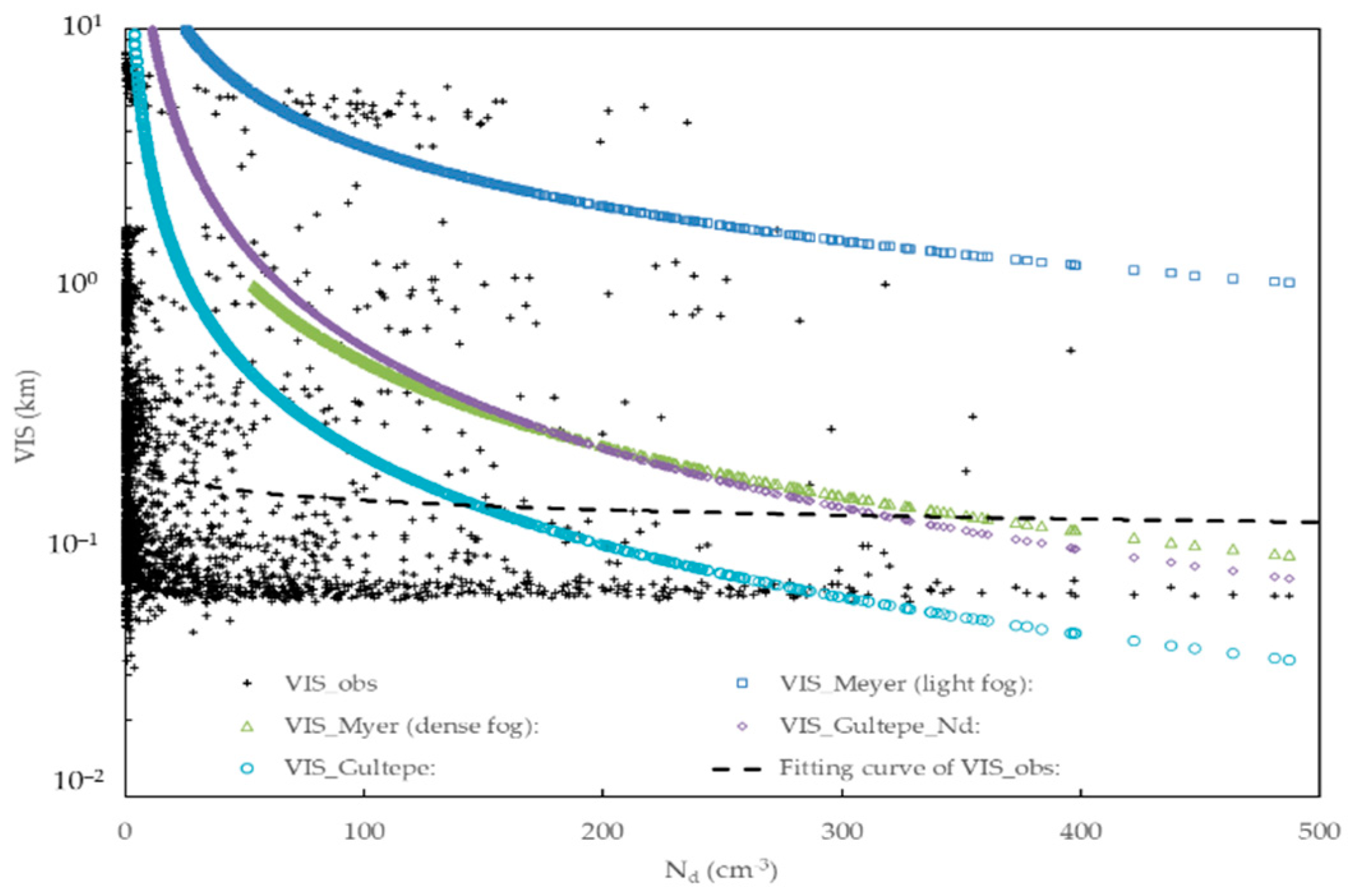
5. Relationships between VIS, N_d, and Fog Droplets Size

In 1980, Meyer et al. [98] proposed that VIS was negatively related to the fog-droplets number concentration and the square of the diameter, and that it varied with the concentration of fog. Therefore, the parameterization schemes of VIS under the thick fog (VIS_MH ≤ 1 km) and the thin mist (VIS_ML > 1–2 km), are obtained, respectively, as follows

$$VI{S}_{MH}=80N_d{}^{-1.1},$$

(21)

and

$$VI{S}_{ML}=120N_d^{-0.77},$$

(22)

where the N_d, which is given in PCS m⁻³, both equations can be applied to the droplet with a diameter of larger than 0.5 μm. Meyer’s observational experiments also showed that the average droplet size essentially remains constant in thin fog, while VIS decreased with increasing droplet size in thick fog, and the formula under the condition of visibility in 1–2 km was $VIS=1.46\times {10}^{-4}{\left(D_e^2\right)}^{-0.49}$, where D_e was the effective diameter of the droplet. Assuming that the scattering coefficient is a constant in the spectrum, the N_d·D_e is proportional to the extinction coefficient. Combined with the relationship between VIS and extinction coefficient,

$$VIS=1.75\times {10}^{-5}{\left(N_d{D}_e^2\right)}^{-0.86}$$

(23)

was obtained, with the slope parameter approaching −1.0. Furthermore, a tiny variation in index results in significant changes of VIS, which might be due to the assumption that the scattering coefficient is a constant and the assumption is valid only for sufficiently large droplets.

The size spectrum of each hydrometeor category is often described by a three-parameter gamma distribution function, $N_d=N_0{D}^{\alpha }{e}^{-\lambda D}$. Two-moment schemes generally treat N₀ and λ as prognostic parameters while maintaining the shape parameter α constant. Milbrandt et al. [99] analyzed the influence of shape parameter α on sedimentation and microphysical growth rate using different schemes. The results show that α plays an important role in determining the rate of size sorting. Kunkel [70] analyzed more than 1400 droplet size samples in 1983, finding a good correlation between the droplet terminal velocity and c (LWC²/N_d)^d (parameter c and d are both fitting coefficients). Under the condition of a fixed LWC value, air pollutants interact with water vapor to form a mass of liquid drops, which increase the N_d. At the same time, a smaller droplet radius decreases the droplet terminal velocity, which results in the deposition rate of liquid water being reduced.

The extinction coefficient increases, and the VIS decreases, due to the increasing average number concentration of droplets associated with the above two physical processes and other chemical processes. Kunkel [70] also indicated that the effect of pollutant concentration in fog should be taken into account. Therefore, the appropriate formulas and droplet terminal velocity should be selected for different polluted conditions. The VIS in fog is affected by the extinction of fog droplets [69,70,76,84], and based on Mie scattering theory, the extinction coefficient is closely related to the Nd. Therefore, the N_d is considered as one of the impact factors of VIS.

In 2006, Gultepe [82] also pointed out that the VIS in fog was not only related to LWC, but also relied on Nd. Result showed that there were differences in the VIS-N_d relationship of the ice fog and liquid fog. The fog was classified into either ice fog (T < −1 °C) or liquid fog (T ≥ −1 °C) on the basis of temperature threshold. Approximate formulas between the VIS, ice fog number concentration (N_i) and liquid fog number concentration (N_d) were obtained through observational analysis and the relationships are as follows:

$$VI{S}_{N_i}=18N_i^{-0.56},$$

(24)

and

$$VI{S}_{N_d}=238N_d^{-1.31},$$

(25)

where the unit of N_i is PCS L⁻¹, and the unit of N_d is PCS cm⁻³, and PCS is the abbreviation of pieces. Gultepe [82] also noted that the results for VIS > 50 km were invalid due to uncertainties in the observation of small droplet by existing instruments. Moreover, on account of the properties of logarithmic relationships, the VIS_Ni, which should be treated cautiously, varied greatly for a given N_i. Based on the observational data from the forward-Scattering Spectrometer in the same year, a new relationship between VIS and N_d was developed by Gultepe [58] as follows:

$$VI{S}_{obs}=44.989N_d^{-1.1592}$$

(26)

Compared with that calculated using Meyers’s expression, the VIS calculated using the new relationship reduced at a faster rate than with the increase of number concentration. Gultepe suggested that the discrepancy may be due to the uncertainty of the number concentration observations in earlier studies or impact factors such as conducting observations in low clouds. The N_d should be treated as an independent variable in parameterization schemes of VIS. Furthermore, in order to establish a more rational parameterization scheme, the accurate monitoring of the number concentration is required.

Based on the observational Nd and VIS_obs data, which were obtained using droplet spectrometer (DMT, FM-120) and VIS meter (Vaisala, PWD 10) in Tianjin [16] from 2016 to 2017, the relationship between VIS and N_d in Tianjin was obtained as the fitting formula: $VIS=0.2522N_d^{-0.121}$ (Figure 3). The constants and exponents parameter of local formula for VIS-N_d relationship is largely different to others. Although a generally decreasing power relationship exists between VIS and N_d, there is still large uncertainty in various regions.

Both the droplet size and the number concentration were not used as a direct output for many previous numerical models. For the droplet size, introducing droplet types and calculating droplet spectra will increase the complexity significantly, while using empirical expressions can simplify the model. For the number concentration, there are no microphysical schemes for the near-surface fog. Even though some numerical models contain microphysical schemes that can directly predict the number concentration, the output of the cloud droplet concentration cannot be treated as the fog-droplets number concentration under the condition of high clouds. The distribution of cloud droplet spectrum is different from that of fog-droplet spectrum; therefore, it is necessary to use the empirical statistical method to estimate the droplets number concentration. For example, N_d is usually given a constant value. Fu G. [6] discussed the performance of the parameterization scheme when N_d = 300 PCS cm⁻³, and showed that the obtained results are significantly smaller than those that do not considering the number concentration.

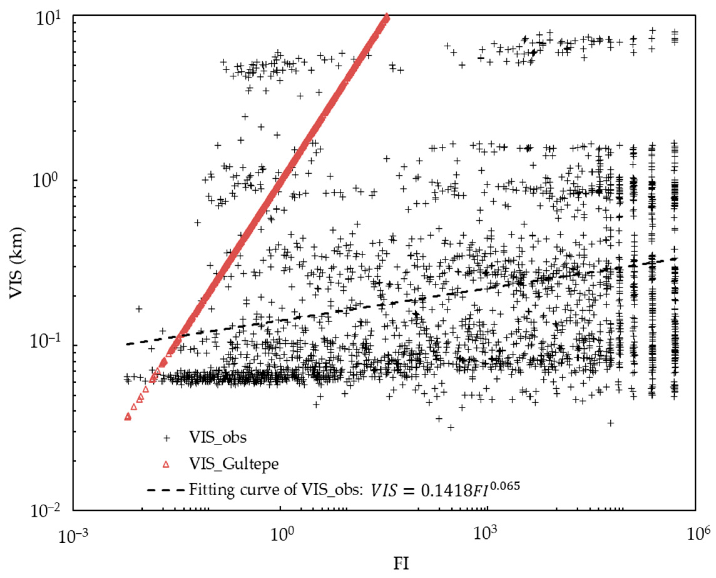
6. Relationships between VIS, LWC and N_d

Based on the descriptions in Section 3 and Section 4, both the LWC and the N_d are considered as the impact factors of VIS; moreover, there is no simple one-to-one relationship between the two factors. For example, the N_d varies over a wide range for a certain LWC, resulting in great differences in VIS. Moreover, the two factors are related to each other. Considering these two main factors at the same time can better reflect the changes of VIS than considering one of them alone [70]. In 2006, based on the previous studies, a new parameterization scheme was established by Gultepe [58], combining the LWC and N_d, t expressed as Equation (27)

$$VIS=1.002/{\left(LWC\times N_d\right)}^{0.6473},$$

(27)

which is suitable for the conditions of 0.005 gm⁻³ < LWC< 0.5 gm⁻³ and 1 cm⁻³ < N_d < 400 cm⁻³. Additionally, a new definition of the fog index (FI) was formulated FI = 1/(LWC*N_d), Compared with Kunkel’s studies [70], Gultepe [58] established a quantitative relational equation, and applied the new scheme to the mesoscale non-hydrostatic model of NOAA. By comparing the results with schemes of K84 and Meyer [98], the results show Equation (27), in which LWC and N_d were taken into account, was more accurate in predicting VIS.

Compared with the K84 scheme, which only considers the LWC, Equation (27) performed better, with significantly lower uncertainty in VIS prediction. While Equation (27) is applied to the Tianjin area (Figure 4), there are still overestimates of VIS over all FI ranges, especially an absence of many low VIS cases in which the FI is large. According to the form of Equation (27), the localized VIS-LWC & N_d formula was fitted as VIS = 0.1418$F{I}^{0.065}$. The local relationship is far lower than in Equation (27), while it has no ability to express some larger VIS. That is to say, even though Equation (27) had done well compared to schemes of K84 and Meyer [98], there is still some work required to promote a parameterized VIS-LWC & Nd relationship in the future.

Hu et al. [100] established a coastal-fog forecast procedure based on the VIS-LWC & N_d parameterization scheme proposed by Gultepe et al. [82]. The LWC was calculated from the physical quantity qcloud output by the WRF model, and the N_d was solved using a historical experience statistical method. The N_d was obtained according to the inversion formula of VIS:$N_d={\mathrm{e}}^{Tmp}$, where $Tmp=\frac{1}{0.6437}\ln \left(\frac{1.002}{VI{S}_{obs}}\right)\ln \left(LW{C}_{obs}\right)$, in which VIS_obs and LWC_obs were the VIS and LWC of similar cases, respectively. The VIS forecast value can be obtained by substituting the obtained LWC and N_d values into the parameterized scheme, which improves the fog forecast accuracy from 61% to 73%, compared with the Stoelinga-Warner scheme [77]. There is also a correlation between LWC and N_d. Gultepe et al. [58] observed that LWC increased with increasing N_d, while the range of N_d changes was very large for a given LWC value. Huang et al. [101] observed and analyzed the microphysical characteristics of sea fog using a droplet spectrometer, finding that an increasing number of droplets with a diameter of more than 10 μm is the main reason for the increase of LWC, while the increase of LWC is the main reason for the decrease of atmospheric VIS under the same N_d interval.

The VIS-LWC & N_d parameterization scheme has certain advantages and a rather high accuracy rate, since both the LWC and N_d are considered, and the microphysical interpretation is relatively more realistic. Similar to the VIS-N_d scheme, it suffers from the same problem of using empirical statistical methods to estimate the concentration of droplets. In addition, the scheme still has a high degree of uncertainty. The research of Gultepe [58] showed that the uncertainty of the scheme for the calculation of VIS in various types of fog still reached 27%. In their study of the characteristics of the fog-droplet spectrum during heavy fog in Tianjin, Liu et al. [52] found that the effects of LWC and N_d on VIS are not the same, and that there was a pronounced negative correlation between VIS and N_d while not so obvious for LWC. Therefore, to better apply the VIS-LWC & N_d relationship obtained by Gultepe et al. [58], the scheme also needs to be improved according to the actual situation in various regions. Song [102] developed a new visibility parameterization by further taking De into the VIS-LWC & N_d relationship consideration at a mountain site in Korea, and indicated that this new parameterization showed better performance than the original VIS-LWC & N_d relationship obtained by Gultepe et al. [58] in visibility value prediction when De was larger than 10 μm, while no obvious improvement was observed when De was less than 10 μm.

In addition, certain correlations still exist among these factors. In order to establish VIS parameterization schemes that are more applicable for the forecast of local VIS, some scholars have carried out the “combination schemes”, which are composed of different parameterization schemes based on the observation data. To solve the problem of abrupt changes in VIS as calculated by LWC scheme, Cao et al. [83] used the localized VIS-RH scheme value to replace discontinuity points in the VIS-LWC scheme. Using 0.05 g kg⁻¹ as the critical lower limit of LWC, Bao et al. [103] simulated cluster fog along the Shanghai-Nanjing Expressway, and used Equation (27) to calculate the value of visibility, and when N_d = 0 or LWC = 0, Equation (27) is found to be no longer applicable, so the VIS-RH scheme is replaced. The results show that in the early stage of heavy fog, the simulated value is lower than the observed value, but the trend of the simulated value and the observed value is consistent during the maintenance and dissipation of the fog. Long et al. [104] determined a combination scheme of VIS-LWC and VIS-RH for the North Coast of Bohai Bay; the results show that if only one scheme is adopted, the simulated VIS value and the measured VIS value will deviate significantly when LWC = 0.03 g/kg. However, the combination scheme behaves well in this condition.

7. Conclusions and Discussion

The characteristics and applications of different parameterization schemes, developed based on various impact factors of VIS, such as RH, extinction coefficient, LWC, and N_d, have been summarized. It can be seen that the fitted parameters, with precise physical meanings, allow for the calculation of VIS by interfacing with numerical forecast products. Therefore, many models are directly interfaced with the corresponding parameterization schemes while postprocessing VIS.

By reviewing the achievements of the VIS parameterization schemes, we understand that none of the current formulas, derived from introducing impact factors or environmental factors, can always accurately calculate the VIS in the fog. It’s important to point out the occurrence and development of fog is the result of multiple processes occurring simultaneously that interact nonlinearly with each other. These interactions likely result in nontrivial sets of key fog parameter values leading to fog formation, while other combinations of values prevent fog formation [105]. Owing to the specific correlations among these factors, the “combination schemes” have also been adopted by many researchers.

The parameterization scheme, which is based on a statistical analysis, has certain shortcomings due to the incomplete consideration of physical processes, and because the physical factors introduced depend on other factors. In fact, the main impact factors vary in different environments, such as the influences of aerosols, as many widely used VIS parameterization schemes are conducted in areas where air pollution is commonly not severe. When applied to fog forecast/simulation in polluted areas, these schemes may overestimate VIS due to the absence of aerosol extinction. For the most commonly used scheme of VIS-LWC, there discrepancies exist between the observed LWC and the model output LWC. The discrepancies in LWC lead to deviations in VIS prediction, and the same problem exists for the observation and data acquisition of RH, N_d, etc. Gultepe et al. [8] point out that further modifications in microphysical observations and parametrizations are needed to promote the fog predictability of numerical-weather-prediction models.

Although existing VIS parameterization schemes have regional limitation, the improvement of the VIS parameterization scheme in the future still required sustained exploration, and it is hoped that a universal scheme can be applied to the atmospheric forecast operation. In addition, with the continuous innovation of computer technology, further studies on the mechanism of different types of fog [106,107], the application of artificial neural network methods [43,108,109,110], and the rapid advance of machine learning and artificial intelligence technologies [111,112], can utilize more tools by which to enhance the accurate numerical calculations of VIS.

VIS parameterization schemes are often highly dependent on the accuracy of the meteorological elements or trigger conditions provided by microphysical schemes [96] or numerical models [95]. When numerical forecast accuracy is not sufficient, even if the VIS parameterization scheme is ideal, the VIS forecast will vary. Some trigger mechanisms or enhancing/limiting processes, such as wind and surrounding buildings, also affect fog prediction accuracy in numerical models [94,97]. Furthermore, the vertical resolution setting has certain influence on fog prediction in the numerical model. Fog can be modeled as different types under the condition of various vertical resolutions [78]. Therefore, it is also important to select the appropriate numerical model for the established parameterization scheme.

References

1. WMO. WMO Guide to Meteorological Instruments and Methods of Observation; Secretariat of the WMO: Geneva, Switzerland, 2006; p. 569. [Google Scholar]
2. Wu, B.G.; Xie, Y.Y.; Wu, D.Z.; Wang, Y.N.; Wang, D.S. Poor visibility on Jingjintang Expressway in autumn/ winter and relevant measures. J. Nat. Disaster 2009, 18, 12–17. (In Chinese) [Google Scholar]
3. Lewis, J.M.; Koracin, D.; Redmond, K.T. Sea Fog Research in the United Kingdom and United States: A Historical Essay Including Outlook. Bull. Am. Meteorol. Soc. 2004, 85, 395–408. [Google Scholar] [CrossRef] [Green Version]
4. Niu, S.J.; Lu, C.S.; Lü, J.J.; Xu, F.; Zhao, L.J.; Liu, D.Y.; Yue, Y.Y.; Zhou, Y.; Yu, H.Y.; Wang, T.S. Advances in fog research in China. Adv. Meteor. Sci. Technol. 2016, 6, 6–19. [Google Scholar]
5. Koračin, D.; Dorman, C.; Lewis, J.M.; Hudson, J.G.; Wilcox, E.; Torregrosa, A. Marine fog: A review. Atmos. Res. 2014, 143, 142–175. [Google Scholar] [CrossRef]
6. Fu, G.; Li, X.L.; Wei, N. Review on the atmospheric visibility research. Period. Ocean. Univ. China 2009, 39, 855–862. (In Chinese) [Google Scholar]
7. Niu, S.; Lu, C.; Yu, H.; Zhao, L.; Lü, J. Fog research in China: An overview. Adv. Atmos. Sci. 2010, 27, 639–662. [Google Scholar] [CrossRef]
8. Gultepe, I.; Heymsfield, A.J.; Fernando, H.J.S.; Pardyjak, E.; Dorman, C.E.; Wang, Q.; Creegan, E.; Hoch, S.W.; Flagg, D.D.; Yamaguchi, R.; et al. A Review of Coastal Fog Microphysics during C-FOG. Boundary-Layer Meteorol. 2021, 181, 1–39. [Google Scholar] [CrossRef]
9. Gultepe, I. Fog and Boundary Layer Clouds: Introduction. Pure Appl. Geophys. 2007, 164, 1115–1116. [Google Scholar] [CrossRef]
10. Laj, P.; Fuzzi, S.; Lazzari, A. The Size Dependent Composition of Fog Droplets. Contrib. Atmos. Phys. 1998, 71, 115–130. [Google Scholar]
11. Frank, G.; Martinsson, B.G.; Cederfelt, S.I. Droplet Formation and Growth in Polluted Fogs. Contrib. Atmos. Phys. 1998, 71, 65–85. [Google Scholar]
12. García-García, F.; Virafuentes, U.; Montero-Martínez, G. Fine-scale measurements of fog-droplet concentrations: A preliminary assessment. Atmos. Res. 2002, 64, 179–189. [Google Scholar] [CrossRef]
13. Hsieh, W.C.; Jonsson, H.; Wang, L.; Buzorius, G.; Flagan, R.C.; Seinfeld, J.H.; Nenes, A. On the representation of droplet coalescence and autoconversion: Evaluation using ambient cloud droplet size distributions. J. Geophys. Res. Atmos. 2009, 114, D07201. [Google Scholar] [CrossRef] [Green Version]
14. Niu, S.; Lu, C.; Liu, Y.; Zhao, L.; Lu, J.; Yang, J. Analysis of the microphysical structure of heavy fog using a droplet spectrometer: A case study. Adv. Atmos. Sci. 2010, 27, 1259–1275. [Google Scholar] [CrossRef]
15. Wang, T.; Niu, S.; Lü, J.; Zhou, Y. Observational Study on the Supercooled Fog Droplet Spectrum Distribution and Icing Accumulation Mechanism in Lushan, Southeast China. Adv. Atmos. Sci. 2019, 36, 29–40. [Google Scholar] [CrossRef]
16. Liu, Q.; Wang, Z.-Y.; Wu, B.-G.; Liu, J.-L.; Nie, H.-H.; Chen, D.-H.; Gultepe, I. Microphysics of fog bursting in polluted urban air. Atmos. Environ. 2021, 253, 1–11. [Google Scholar] [CrossRef]
17. Fuzzi, S.; Facchini, M.C.; Orsi, G.; Bonforte, G.; Martinotti, W.; Ziliani, G.; Mazzalit, P.; Rossi, P.; Natale, P.; Grosa, M.M.; et al. The NEVALPA project: A regional network for fog chemical climatology over the PO Valley basin. Atmos. Environ. 1996, 30, 201–213. [Google Scholar] [CrossRef]
18. Ma, C.-J.; Kasahara, M.; Tohno, S.; Sakai, T. A replication technique for the collection of individual fog droplets and their chemical analysis using micro-PIXE. Atmos. Environ. 2003, 37, 4679–4686. [Google Scholar] [CrossRef]
19. Mancinelli, V.; Decesari, S.; Emblico, L.; Tozzi, R.; Mangani, F.; Fuzzi, S.; Facchini, M.C. Extractable iron and organic matter in the suspended insoluble material of fog droplets. Water Air Soil Pollut. 2006, 174, 303–320. [Google Scholar] [CrossRef]
20. Raja, S.; Raghunathan, R.; Yu, X.-Y.; Lee, T.; Chen, J.; Kommalapati, R.R.; Murugesan, K.; Shen, X.; Qingzhong, Y.; Valsaraj, K.T.; et al. Fog chemistry in the Texas–Louisiana Gulf Coast corridor. Atmos. Environ. 2008, 42, 2048–2061. [Google Scholar] [CrossRef]
21. Li, Z.; Liu, D.; Yan, W.; Wang, H.; Zhu, C.; Zhu, Y.; Zu, F. Dense fog burst reinforcement over Eastern China: A review. Atmos. Res. 2019, 230, 104639. [Google Scholar] [CrossRef]
22. Roach, W.T. Effective of Radiative Exchange on Growth by Consideration of a Cloud or Fog Droplet. Q. J. R. Meteorol. Soc. 1976, 102, 361–372. [Google Scholar] [CrossRef]
23. Guo, L.; Guo, X.; Fang, C.; Zhu, S. Observation analysis on characteristics of formation, evolution and transition of a long-lasting severe fog and haze episode in North China. Sci. China Earth Sci. 2015, 58, 329–344. [Google Scholar] [CrossRef]
24. Oliver, D.A.; Lewellen, W.S.; Williamson, G.G. The interaction between turbulent and radiative transport in the development of fog and low level stratus. J. Atmos. Sci. 1978, 35, 301–316. [Google Scholar]
25. Wu, B.G.; Zhang, H.S.; Zhang, C.C.; Zhu, H.; Wang, Z.Y.; Xie, Y.Y. Characteristics of turbulent transfer and its temporal evolution during an advection fog period in North China. Chin. J. Atmos. Sci. 2010, 34, 440–448. (In Chinese) [Google Scholar]
26. Ye, X.; Wu, B.; Zhang, H. The turbulent structure and transport in fog layers observed over the Tianjin area. Atmos. Res. 2015, 153, 217–234. [Google Scholar] [CrossRef]
27. Wu, B.; Li, Z.; Ju, T.; Zhang, H. Characteristics of Low-level jets during 2015–2016 and the effect on fog in Tianjin. Atmos. Res. 2020, 245, 105102. [Google Scholar] [CrossRef]
28. Kim, C.K.; Yum, S.S. A study on the transition mechanism of a stratus cloud into a warm sea fog using a single column model PAFOG coupled with WRF. Asia-Pacific J. Atmos. Sci. 2013, 49, 245–257. [Google Scholar] [CrossRef]
29. Hu, H.; Sun, J.; Zhang, Q. Assessing the Impact of Surface and Wind Profiler Data on Fog Forecasting Using WRF 3DVAR: An OSSE Study on a Dense Fog Event over North China. J. Appl. Meteorol. Clim. 2017, 56, 1059–1081. [Google Scholar] [CrossRef] [Green Version]
30. Gilson, G.F.; Jiskoot, H.; Cassano, J.J.; Gultepe, I.; James, T.D. The Thermodynamic Structure of Arctic Coastal Fog Occurring During the Melt Season over East Greenland. Boundary-Layer Meteorol. 2018, 168, 443–467. [Google Scholar] [CrossRef]
31. Ju, T.; Wu, B.; Zhang, H.; Liu, J. Characteristics of turbulence and dissipation mechanism in a polluted radiation–advection fog life cycle in Tianjin. Meteorol. Atmos. Phys. 2020, 133, 515–531. [Google Scholar] [CrossRef]
32. Shi, C.; Roth, M.; Zhang, H.; Li, Z. Impacts of urbanization on long-term fog variation in Anhui Province, China. Atmos. Environ. 2008, 42, 8484–8492. [Google Scholar] [CrossRef]
33. Tian, M.; Wu, B.G.; Huang, H.; Wang, Z.W.; Zhang, W.Y. The synoptic condition and boundary layer characteristics of coastal fog around the Bohai Sea. Climatic Environ. Res. 2020, 25, 199–210. (In Chinese) [Google Scholar]
34. Li, Q.; Wub, B.; Liu, J.; Zhang, H.; Cai, X.; Song, Y. Characteristics of the atmospheric boundary layer and its relation with PM2:5 during haze episodes in winter in the North China Plain. Atmos. Environ. 2020, 223, 1–10. [Google Scholar] [CrossRef]
35. Huang, H.; Liu, H.; Huang, J.; Mao, W.; Bi, X. Atmospheric Boundary Layer Structure and Turbulence during Sea Fog on the Southern China Coast. Mon. Weather. Rev. 2015, 143, 1907–1923. [Google Scholar] [CrossRef]
36. Bergot, T.; Escobar, J.; Masson, V. Effect of small-scale surface heterogeneities and buildings on radiation fog: Large-eddy simulation study at Paris-Charles de Gaulle airport. Q. J. R. Meteorol. Soc. 2015, 141, 285–298. [Google Scholar] [CrossRef]
37. Gultepe, I. Fog and Boundary Layer Clouds: Fog Visibility and Forecasting; Birkhäuser Verlag AG: Basel, Switzerland, 2008. [Google Scholar]
38. Roquelaure, S.; Bergot, T. A Local Ensemble Prediction System for Fog and Low Clouds: Construction, Bayesian Model Averaging Calibration, and Validation. J. Appl. Meteorol. Clim. 2008, 47, 3072–3088. [Google Scholar] [CrossRef]
39. Ryerson, W.R.; Hacker, J.P. The Potential for Mesoscale Visibility Predictions with a Multimodel Ensemble. Weather. Forecast. 2014, 29, 543–562. [Google Scholar] [CrossRef]
40. Lin, J.C.-H.; Tai, J.-H.; Feng, C.-H.; Lin, D.-E. Towards Improving Visibility Forecasts in Taiwan: A Statistical Approach. Terr. Atmos. Ocean. Sci. 2010, 21, 359–374. [Google Scholar] [CrossRef] [Green Version]
41. Leyton, S.M.; Fritsch, J.M. Short-Term Probabilistic Forecasts of Ceiling and Visibility Utilizing High-Density Surface Weather Observations. Weather. Forecast. 2003, 18, 891–902. [Google Scholar] [CrossRef]
42. Ryerson, W.R.; Hacker, J.P. A Nonparametric Ensemble Postprocessing Approach for Short-Range Visibility Predictions in Data-Sparse Areas. Weather. Forecast. 2018, 33, 835–855. [Google Scholar] [CrossRef]
43. Pasini, A.; Pelino, V.; Potestà, S. A neural network model for visibility nowcasting from surface observations: Results and sensitivity to physical input variables. J. Geophys. Res. Space Phys. 2001, 106, 14951–14959. [Google Scholar] [CrossRef]
44. Roquelaure, S.; Tardif, R.; Remy, S.; Bergot, T. Skill of a Ceiling and Visibility Local Ensemble Prediction System (LEPS) according to Fog-Type Prediction at Paris-Charles de Gaulle Airport. Weather. Forecast. 2009, 24, 1511–1523. [Google Scholar] [CrossRef] [Green Version]
45. Zhou, B.; Du, J. Fog Prediction from a Multimodel Mesoscale Ensemble Prediction System. Weather. Forecast. 2010, 25, 303–322. [Google Scholar] [CrossRef]
46. Hansen, B. A Fuzzy Logic–Based Analog Forecasting System for Ceiling and Visibility. Weather. Forecast. 2007, 22, 1319–1330. [Google Scholar] [CrossRef]
47. Zhou, B.; Ferrier, B.S. Asymptotic Analysis of Equilibrium in Radiation Fog. J. Appl. Meteorol. Clim. 2008, 47, 1704–1722. [Google Scholar] [CrossRef]
48. Sohoni, V.V.; Paranjpe, M.M. Fog and relative humidity in India. Q. J. R. Meteorol. Soc. 1934, 60, 15–22. [Google Scholar] [CrossRef]
49. Francis, K.E. Study of ice fog particles in alaska. Bull. Am. Meteorol. Soc. 1962, 43, 139. [Google Scholar]
50. Li, X.N.; Huang, J.A.; Shen, S.H.; Liu, S.D.; Lu, W.H. Evolution of Liquid Water Content in a Sea Fog Controlled by a High-Pressure Pattern. J. Trop. Meteorol. 2010, 16, 409–416. [Google Scholar] [CrossRef]
51. Liu, D.Y.; Pu, M.J.; Yang, J.; Zhang, G.Z.; Yan, W.L.; Li, Z.H. Microphysical Structure and Evolution of a Four-Day Persistent Fog Event in Nanjing in December 2006. Acta Meteorol. Sin. 2009, 24, 104–115. [Google Scholar]
52. Liu, Q.; Wu, B.; Wang, Z.; Hao, T. Fog Droplet Size Distribution and the Interaction between Fog Droplets and Fine Particles during Dense Fog in Tianjin, China. Atmosphere 2020, 11, 258. [Google Scholar] [CrossRef] [Green Version]
53. Steeneveld, G.J.; Ronda, R.J.; Holtslag, A.A.M. The Challenge of Forecasting the Onset and Development of Radiation Fog Using Mesoscale Atmospheric Models. Boundary-Layer Meteorol. 2015, 154, 265–289. [Google Scholar] [CrossRef]
54. Singh, A.; George, J.P.; Iyengar, G.R. Prediction of fog/visibility over India using NWP Model. J. Earth Syst. Sci. 2018, 127, 26. [Google Scholar] [CrossRef] [Green Version]
55. Philip, A.; Bergot, T.; Bouteloup, Y.; Bouyssel, F. The Impact of Vertical Resolution on Fog Forecasting in the Kilometric-Scale Model AROME: A Case Study and Statistics. Weather. Forecast. 2016, 31, 1655–1671. [Google Scholar] [CrossRef]
56. Tian, M.; Wu, B.; Huang, H.; Zhang, H.; Zhang, W.; Wang, Z. Impact of water vapor transfer on a Circum-Bohai-Sea heavy fog: Observation and numerical simulation. Atmos. Res. 2019, 229, 1–22. [Google Scholar] [CrossRef]
57. Price, J.D.; Lane, S.; Boutle, I.; Smith, D.K.E.; Bergot, T.; Lac, C.; Duconge, L.; McGregor, J.; Kerr-Munslow, A.; Pickering, M.; et al. LANFEX: A Field and Modeling Study to Improve Our Understanding and Forecasting of Radiation Fog. Bull. Am. Meteorol. Soc. 2018, 99, 2061–2077. [Google Scholar] [CrossRef]
58. Gultepe, I.; Müller, M.D.; Boybeyi, Z. A New Visibility Parameterization for Warm-Fog Applications in Numerical Weather Prediction Models. J. Appl. Meteorol. Clim. 2006, 45, 1469–1480. [Google Scholar] [CrossRef]
59. Porson, A.; Price, J.; Lock, A.; Clark, P. Radiation Fog. Part II: Large-Eddy Simulations in Very Stable Conditions. Boundary-Layer Meteorol. 2011, 139, 193–224. [Google Scholar] [CrossRef]
60. Kim, C.K.; Stuefer, M.; Schmitt, C.G.; Heymsfield, A.; Thompson, G. Numerical Modeling of Ice Fog in Interior Alaska Using the Weather Research and Forecasting Model. Pure Appl. Geophys. 2014, 171, 1963–1982. [Google Scholar] [CrossRef]
61. Koračin, D. Modeling and Forecasting Marine Fog. In Marine Fog: Challenges and Advancements in Observations, Modeling, and Forecasting; Koračin, D., Dorman, C.E., Eds.; Springer International Publishing: Cham, Switzerland, 2017; pp. 425–475. [Google Scholar]
62. Koschmieder, H. Theorie der horizontalen Sichtweite. Beitr. Phys. Fr. Atmos. 1924, 12, 33–53. [Google Scholar]
63. Malone, T. Compendium of Meteorology; American Meteorological Society: Boston, MA, USA, 1951. [Google Scholar]
64. Houghton, H.G.; Radford, W.H. On the measurement of drop size and liquid water content in fogs and clouds. Phys. Oceanogr. Meteorol. 1938, 6, 1–31. [Google Scholar] [CrossRef] [Green Version]
65. Eldridge, R.G. The Relationship Between Visibility and Liquid Water Content in Fog. Atmos. Sci. 1971, 8, 1183–1186. [Google Scholar] [CrossRef] [Green Version]
66. Horvath, H. On the applicability of the koschmieder visibility formula. Atmos. Environ. 1967 1971, 5, 177–184. [Google Scholar] [CrossRef]
67. Lee, Z.; Shang, S. Visibility: How applicable is the century-old Koschmieder model? J. Atmos. Sci. 2016, 73, 4573–4581. [Google Scholar] [CrossRef]
68. Mie, V.G. Consideraciones sobre la óptica de los medios turbios, especialmente soluciones coloidales. Por Gustav Mie Ann. Der Phys. 1908, 25, 377–445. [Google Scholar] [CrossRef]
69. Koenig, L.R. Numerical experiments pertaining to warm-fog clearing. Mon. Weather. Rev. 1971, 99, 227–241. [Google Scholar] [CrossRef] [Green Version]
70. Kunkel, B.A. Parameterization of Droplet Terminal Velocity and Extinction Coefficient in Fog Models. J. Clim. Appl. Meteorol. 1984, 23, 34–41. [Google Scholar] [CrossRef] [Green Version]
71. ECWMF. IFS DOCUMENTATION–Cy47r3, Operational Implementation. PART IV: PHYSICAL PROCESSES; European Centre for Medium-Range Weather Forecasts: Shinfield Park, Reading, RG2 9AX, UK. 12 October 2021. Available online: https://www.ecmwf.int/sites/default/files/elibrary/2021/20198-ifs-documentation-cy47r3-part-vi-physical-processes.pdf (accessed on 8 December 2021).
72. Clark, P.A.; Harcourt, S.A.; Macpherson, B.; Mathison, C.T.; Cusack, S.; Naylor, M. Prediction of visibility and aerosol within the operational Met Office Unified Model. I: Model formulation and variational assimilation. Q. J. R. Meteorol. Soc. 2008, 134, 1801–1816. [Google Scholar] [CrossRef] [Green Version]
73. Gao, S.; Lin, H.; Shen, B.; Fu, G. A heavy sea fog event over the Yellow Sea in March 2005: Analysis and numerical modeling. Adv. Atmos. Sci. 2007, 24, 65–81. [Google Scholar] [CrossRef]
74. Fu, G.; Guo, J.; Pendergrass, A.; Li, P. An analysis and modeling study of a sea fog event over the Yellow and Bohai Seas. J. Ocean Univ. China 2008, 7, 27–34. [Google Scholar] [CrossRef]
75. Fu, G.; Guo, J.; Xie, S.-P.; Duan, Y.; Zhang, M. Analysis and high-resolution modeling of a dense sea fog event over the Yellow Sea. Atmos. Res. 2006, 81, 293–303. [Google Scholar] [CrossRef]
76. Vali, G.; Politovich, M.K.; Baumgardner, D.G. Conduct of Cloud Spectra Measurements; Air Force Geophysics Laboratory, Wright-Patterson AFB: Fairborn, OH, USA, 1979; pp. 1–61. [Google Scholar]
77. Stoelinga, M.T.; Warner, T.T. Nonhydrostatic, Mesobeta-Scale Model Simulations of Cloud Ceiling and Visibility for an East Coast Winter Precipitation Event. J. Atmos. Sci. 1999, 38, 385–404. [Google Scholar] [CrossRef]
78. Elias, T.; Haeffelin, M.; Drobinski, P.; Gomes, L.; Rangognio, J.; Bergot, T.; Chazette, P.; Raut, J.-C.; Colomb, M. Particulate contribution to extinction of visible radiation: Pollution, haze, and fog. Atmos. Res. 2009, 92, 443–454. [Google Scholar] [CrossRef]
79. van Oldenborgh, G.J.; Yiou, P.; Vautard, R. On the roles of circulation and aerosols in the decline of mist and dense fog in Europe over the last 30 years. Atmos. Chem. Phys. Discuss. 2010, 10, 4597–4609. [Google Scholar] [CrossRef] [Green Version]
80. Hänel, G. The Properties of Atmospheric Aerosol Particles as Functions of the Relative Humidity at Thermodynamic Equilibrium with the Surrounding Moist Air. Adv. Geophys. 1976, 19, 73–188. [Google Scholar] [CrossRef]
81. Smirnova, T.G.; Benjamin, S.G.; Brown, J.M. Case study verification of RUC/ MAPS fog and visibility forecasts. In Preprints, 9th Conference on Aviation, Range, and Aerospace Meteorology; AMS: Orlando, FL, USA, 2000; pp. 31–36. [Google Scholar]
82. Gultepe, I.; Isaac, G.A. Visibility Versus Precipitation Rate and Relative Humidity. In Proceedings of the Wisconsin: Meteor. Soc., 2006; P2.55. 12th Cloud Physics Conf. Madison, Amer. 12 July 2006. Available online: http://ams.confex.com/ams/Madison2006/techprogram/paper_113177.htm (accessed on 8 December 2021).
83. Cao, X.C.; Shao, L.M.; Li, X.D. Research on parameterization scheme of visibility in Fog Model. In Proceedings of the 31st Annual Meeting of the Chinese Meteorological Society, Beijing, China, 3 November 2014; 2014; pp. 1–5. [Google Scholar]
84. Gültepe, I.; Milbrandt, J.A. Probabilistic Parameterizations of Visibility Using Observations of Rain Precipitation Rate, Relative Humidity, and Visibility. J. Appl. Meteorol. 2009, 49, 36–46. [Google Scholar] [CrossRef]
85. Lin, Y.; Wang, M.S.; Lin, L.G. Numerical simulation of a winter fog in Sichuan and parameterization of visibility. J. Nanjing Univ. Inf. Sci. Technol. Nat. Sci. Ed. 2013, 5, 222–228. [Google Scholar]
86. Roquelaure, S.; Bergot, T. Contributions from a Local Ensemble Prediction System (LEPS) for Improving Fog and Low Cloud Forecasts at Airports. Weather. Forecast. 2009, 24, 39–52. [Google Scholar] [CrossRef] [Green Version]
87. Lin, Y.; Yang, J.; Bao, Y.S.; Wang, Z.J.; Dai, Y.X. The numerical simulation of visibility during the fog in Shanxi province in winter. J. Nanjing Univ. Inf. Sci. Technol. Nat. Sci. Ed. 2010, 2, 436–444. [Google Scholar]
88. Bari, D. A Preliminary Impact Study of Wind on Assimilation and Forecast Systems into the One-Dimensional Fog Forecasting Model COBEL-ISBA over Morocco. Atmosphere 2019, 10, 615. [Google Scholar] [CrossRef] [Green Version]
89. Martinet, P.; Cimini, D.; Burnet, F.; Ménétrier, B.; Michel, Y.; Unger, V. Improvement of numerical weather prediction model analysis during fog conditions through the assimilation of ground-based microwave radiometer observations: A 1D-Var study. Atmos. Meas. Tech. 2020, 13, 6593–6611. [Google Scholar] [CrossRef]
90. Eldridge, R.G. Haze and Fog Aerosol Distributions. J. Atmos. Sci. 1966, 23, 605–613. [Google Scholar] [CrossRef] [Green Version]
91. Tomasi, C.; Tampieri, F. Features of the proportionality coefficient in the relationship between visibility and liquid water content in haze and fog. Atmosphere 1976, 14, 61–76. [Google Scholar] [CrossRef] [Green Version]
92. Pinnick, R.G.; Hoihjelle, D.L.; Fernandez, G.; Stenmark, E.B.; Lindberg, J.D.; Hoidale, G.B.; Jennings, S.G. Vertical Structure in Atmospheric Fog and Haze and Its Effects on Visible and Infrared Extinction. J. Atmos. Sci. 1978, 35, 2020–2032. [Google Scholar] [CrossRef] [Green Version]
93. Musson-Genon, L. Numerical Simulation of a Fog Event with a One-Dimensional Boundary Layer Model. Mon. Weather. Rev. 1987, 115, 592–607. [Google Scholar] [CrossRef]
94. Wang, Q.; Zhang, S.-P.; Wang, Q.; Meng, Z.-X.; Koračin, D.; Gao, S.-H. A Fog Event off the Coast of the Hangzhou Bay during Meiyu Period in June 2013. Aerosol Air Qual. Res. 2018, 18, 91–102. [Google Scholar] [CrossRef] [Green Version]
95. Singh, A.; Dey, S. Influence of aerosol composition on visibility in megacity Delhi. Atmos. Environ. 2012, 62, 367–373. [Google Scholar] [CrossRef]
96. Shen, X.J.; Sun, J.Y.; Zhang, X.Y.; Zhang, Y.M.; Zhang, L.; Che, H.C.; Ma, Q.L.; Yu, X.M.; Yue, Y.; Zhang, Y.W. Characterization of submicron aerosols and effect on visibility during a severe haze-fog episode in Yangtze River Delta, China. Atmos. Environ. 2015, 120, 307–316. [Google Scholar] [CrossRef] [Green Version]
97. Gonser, S.G.; Klemm, O.; Griessbaum, F.; Chang, S.-C.; Chu, H.-S.; Hsia, Y.-J. The Relation Between Humidity and Liquid Water Content in Fog: An Experimental Approach. Pure Appl. Geophys. 2011, 169, 821–833. [Google Scholar] [CrossRef]
98. Meyer, M.B.; Jiusto, J.E.; Lala, G.G. Measurements of Visual Range and Radiation-Fog (Haze) Microphysics. J. Atmos. Sci. 1980, 37, 622–629. [Google Scholar] [CrossRef] [Green Version]
99. Milbrandt, J.A.; Yau, M.K. A Multimoment Bulk Microphysics Parameterization. Part I: Analysis of the Role of the Spectral Shape Parameter. J. Atmos. Sci. 2005, 62, 3051–3064. [Google Scholar] [CrossRef] [Green Version]
100. Hu, B.; Du, H.L.; Hao, S.F.; Yu, L.M.; Teng, L.N. A forecast method of coastal sea fog based on the combination of statistic technique and dynamical interpretation. Marin. Forec. 2014, 31, 82–86. (In Chinese) [Google Scholar]
101. Huang, H.J.; Huang, J.; Mao, W.K.; Liao, F.; Li, X.N.; Lü, W.H.; Yang, Y.Q. Characteristics of liquid water content of sea fog in Maoming area and its relationship with atmospheric horizontal visibility. Acta Oceanol. Sin. 2010, 32, 40–52. (In Chinese) [Google Scholar]
102. Song, J.I.; Yum, S.S.; Gultepe, I.; Chang, K.-H.; Kim, B.-G. Development of a new visibility parameterization based on the measurement of fog microphysics at a mountain site in Korea. Atmos. Res. 2019, 229, 115–126. [Google Scholar] [CrossRef]
103. Bao, Y.X.; Ding, Q.J.; Yuan, C.S.; Yan, M.L. Numerical simulations of a highly complex fog event on Shanghai-Nanjing Expressway. Chin. J. Atmos. Sci. 2013, 37, 124–136. (In Chinese) [Google Scholar]
104. Long, Q.; Wang, F.; Mi, X.Y.; Wang, C.; Liu, Y. Research on the Formation Mechanism and Forecast Technology of Sea Fog on the North Coast of Bohai Bay. In Proceedings of the 2020 National Marine Ecological Environmental Protection and Monitoring Technology Symposium, Shenzhen, China, 18 December 2020; pp. 238–246. [Google Scholar]
105. Haeffelin, M.; Bergot, T.; Elias, T.; Tardif, R.; Carrer, D.; Chazette, P.; Colomb, M.; Drobinski, P.; Dupont, E.; Dupont, J.-C.; et al. Parisfog Shedding New Light on Fog Physical Processes. Bull. Am. Meteorol. Soc. 2010, 91, 767–783. [Google Scholar] [CrossRef] [Green Version]
106. Li, Z.H.; Peng, Z.G. Physical and chemical characteristic of the Chongqing winter fog. Acta. Meteorol. Sin. 1994, 16, 46–54. (In Chinese) [Google Scholar]
107. Sun, J.; Huang, H.; Zhang, S.; Mao, W. How Sea Fog Influences Inland Visibility on the Southern China Coast. Atmosphere 2018, 9, 344. [Google Scholar] [CrossRef] [Green Version]
108. Marzban, C.; Leyton, S.; Colman, B. Ceiling and Visibility Forecasts via Neural Networks. Weather. Forecast. 2007, 22, 466–479. [Google Scholar] [CrossRef] [Green Version]
109. Gilleland, E.; Fowler, T.L. Network design for verification of ceiling and visibility forecasts. Environmetrics 2006, 17, 575–589. [Google Scholar] [CrossRef]
110. Fabbian, D.; de Dear, R.; Lellyett, S. Application of artificial neural network forecasts to predict fog at Canberra International Airport. Weather. Forecast. 2007, 22, 372–381. [Google Scholar] [CrossRef]
111. Bari, D.; Ouagabi, A. Machine-learning regression applied to diagnose horizontal visibility from mesoscale NWP model forecasts. SN Appl. Sci. 2020, 2, 1–13. [Google Scholar] [CrossRef] [Green Version]
112. Bingui, W.; Jianchun, Z.; Yinghua, L.; Yanan, W.; Mei, X.; Jing, C.; Xuelian, W.; un, G.X.; Xiaobin, Q. Research on Numerical Interpretative Forecast for Low-Visibility at Tianjin Port in Autumn and Wint. Meteorol. Mon. 2017, 43, 8630871. [Google Scholar]
Figure 1. Performance of VIS-RH schemes in Tianjin (VIS_Eq.7… VIS_Eq.16 denote Equation (7) to (16), and the black dashed line denotes the localized fitting curve of VIS-RH).
Atmosphere 12 01666 g001
Figure 2. VIS-LWC scheme verified and the local fitting formula and the VIS less than 1 km (a) and the wide-range VIS data (b) (VIS_obs, VIS_K84, VIS_Gultepe, fitting curve of VIS represent the observed VIS, simulated VIS with Equation (19), Equation (20) and the local fitting, respectively).
Atmosphere 12 01666 g002
Figure 3. VIS-Nd scheme performance evaluation (VIS_Meyer (light fog) /VIS_Meyer (dense fog), VIS_Gultepe_Nd, VIS_Gultepe represent simulated VIS from Equation (22), (21), (26), and (25), respectively. The black dashed line denotes the localized fitting curve of VIS-Nd from local VIS_obs).
Atmosphere 12 01666 g003
Figure 4. VIS-fog index (FI = 1/Nd*LWC) scheme calculation (The black dashed line denotes the fitting curve of VIS_obs, VIS_Gultepe denotes denotes Equation (27), respectively).
Atmosphere 12 01666 g004