Article

Distinguishing Time Scales of Katabatic Flow in Complex Terrain

1
Department of Physics, University of Nevada, Reno, Reno, NV 89512, USA
2
Biological and Ecological Engineering Department, Oregon State University, Corvallis, OR 97331, USA
3
Department of Mechanical Engineering, University of Utah, Salt Lake City, UT 84112, USA
*
Author to whom correspondence should be addressed.
Atmosphere 2021, 12(12), 1651; https://doi.org/10.3390/atmos12121651
Submission received: 14 October 2021 / Revised: 6 December 2021 / Accepted: 6 December 2021 / Published: 9 December 2021
(This article belongs to the Section Biosphere/Hydrosphere/Land–Atmosphere Interactions)

Abstract

:
To examine spatial and temporal scales of katabatic flow, a distributed temperature sensing (DTS) optical fiber was deployed 2 km down a mild slope irregularly interrupted by small-scale drainage features as part of the Mountain Terrain Atmospheric Modeling and Observation (MATERHORN) experiment conducted at the U.S. Army Dugway Proving Ground, Utah. The fiber was suspended at two heights near the surface, enabling measurement of variations in lapse rate near the surface at meter-scale spatial resolution with 1-min temporal resolution. Experimental results derived from the DTS and tower-mounted instrumentation indicate that airflow through small-scale drainage features regulated the local cooling rate whereas topographic slope and distance along the drainage strongly influenced the larger-scale cooling rate. Empirical results indicate that local cooling rate decays exponentially after local sunset and basin-wide cooling rate decreases linearly with time. The difference in the functional form for cooling rate between local and basin-wide scales suggests that small-scale features have faster timescales that manifests most strongly shortly after local sunset. More generally, partitioning drainage flow by scale provides insight and a methodology for improved understanding of drainage flow in complex terrain.

1. Introduction

During the clear sky transition from day to night, longwave surface cooling begins to exceed warming by solar insolation and the earth’s surface temperature decreases. Radiant cooling on sloped terrain cools the air just above it, initiating downslope flow, referred to as a katabatic wind or “drainage flow” [1,2]. Fundamentally, air cooled near the surface obtains sufficient density to become negatively buoyant and air flows downhill despite warming by adiabatic compression. When synoptic forcing is weak, nocturnal katabatic winds can enhance the development of persistent cold air pools that exacerbate air pollution [3,4,5], crop mortality [6,7] and transportation hazards [8,9,10].
Laboratory and field-based experiments have identified numerous environmental factors that influence the expression of katabatic flow across both idealized and complex landscapes. These environmental factors include spatial measures, such as slope, elevation, aspect, and surface roughness, as well as spatio-temporal measures of ambient atmospheric conditions and surface energy balance (SEB) [11]. Previous field studies utilized towers, tethered balloons, aircraft, and combinations of these platforms to host instrumentation that acquired temperature and velocity profiles of katabatic flow [12]. A common shortcoming of these experiments, however, has been that instrument spacing has been inadequate to resolve the broad range of time scales of the evolving near-surface temperature field that drives katabatic flows.
Model simulations provide an alternate approach for examining katabatic flow development. With model simulations, one can reduce the set of environmental factors that contribute to katabatic flow and thereby glean understanding that would be difficult to obtain in a field-based setting [13,14,15,16,17]. Yet, despite the increase in spatial and temporal granularity afforded by ever-increasing computational power, models remain limited in the mix of spatial and temporal scales they can simulate [18]. These limitations lead to, for example, underestimating both scalar field heterogeneity and the effect of subgrid-scale gradients [19]. Since the buoyancy force driving katabatic wind is strongest near the surface, resolving the temperature deficit of air just above the surface is critical for discerning the range of temporal scales of motion for katabatic flow.
Distributed temperature sensing (DTS) provides a synergistic technique for studying katabatic flow with capabilities unfulfilled by tower-based instrumentation, lidar, and model simulations. A DTS deployment can obtain precise temperature measurements at sub-minute temporal resolution and sub-meter spatial resolution over a multi-kilometer extent [20]. Compared with lidar, one prominent limitation of DTS is that measurements are obtained along an optical fiber segment rather than volume averaged. Therefore, the fiber deployment topology must be well-considered to appropriately test an experimental hypothesis. Nevertheless, DTS capabilities enable novel hypothesis testing of the influence that spatial measures, such as slope and downrange distance, have on katabatic flow evolution. With DTS, we examine several questions based on how fine-scale surface features impact the formation of near-surface vertical temperature gradients, local cooling rates, and advection, as well as the most important spatial measures for a given topographic scenario (e.g., slope, relative position, elevation).
The interdependency between spatial and temporal scales for katabatic wind response was a motivating factor in designing the Mountain Terrain Atmospheric Modeling and Observation (MATERHORN) project [21]. Similar to a modeling approach, the MATERHORN project constrained the set of causal environmental factors by focusing on an arid environment, thereby reducing biotic impacts on sensible and latent heat fluxes. Results from MATERHORN published in [11] utilized tower-mounted instruments to characterize various elements of katabatic flow. However, [11] lacked the spatial resolution needed to examine the fine-grained temperature evolution of katabatic winds. In contrast to a comparative katabatic flow experiment near La Fouly, Switzerland [22], the experiment location in this study is characterized by topographic undulations and small-scale drainage features, enabling flow characterization over a broad range of spatial and temporal scales.
In this manuscript, we examine, in detail, how the temperature field of katabatic flow evolves as a function of relevant spatial measures, such as slope, distance downslope (range), and proximity to drainage features. We test the hypothesis that terrain complexity produces a range of time scales of katabatic flow response and the functional form of katabatic flow varies with spatial scale. The experiment site and methods are described in Section 2. In Section 3.1, tower data are used to identify synoptic influences and subset data to periods with minimal synoptic forcing. DTS timeseries identify near-surface temperature gradients as a function of position on the slope. In Section 3.2, trends in near-surface temperature lapse rate are distinguished as functions of position relative to topographic features and downrange distance. Near-surface cooling rates are examined as a function of height, slope, and range in Section 3.3. Coefficients for an empirically-derived prognostic equation that describes near-surface katabatic flow evolution are estimated in Section 4.

2. Materials and Methods

We deployed a DTS system at two heights across a 2-km transect with a mild slope, little vegetation, and irregularly interrupted by small-scale drainage features (Figure 1). The DTS system was deployed from 28 September through 21 October 2012 on the east slope of Granite Peak at the U.S. Army Dugway Proving Ground, Utah. Starting ~100 m east of tower ES2 (elevation 1351 m), the optical fiber was deployed uphill past tower ES5 (elevation 1440 m) at 1.0 m ± 0.05 m height a.g.l. and then back downhill to ES2 at 0.5 m ± 0.05 m a.g.l. At each of the two heights (0.5 and 1 m), the optical fiber was placed in the slit of foam blocks that were affixed with zip ties to rebar stakes spaced nominally at 10-m intervals. Foam blocks minimized spurious temperature spikes due to the difference in heat capacity between rebar and the air. In all, the DTS system was deployed over a 23-day period but it was overrun twice by wild horses (an atypical objective danger). Hence, in total, new fiber lines were deployed three times. In this paper, we present data acquired between 7 October and 14 October 2014.
To date, DTS technology has been used for hydrologic [23,24], soil [25,26], and atmospheric science applications [27,28,29]. However, DTS is not commonly used; thus, a brief overview of its operation is required. The primary components of a DTS are a base station that emits monochromatic light pulses and an optical fiber through which the light pulses traverse. As a light pulse traverses the fiber a small fraction of light backscatters by Raman scattering. For a given emitted frequency, Raman scattering produces weak peaks in amplitude on either side of the centerline of emitted wavelength, called the Stokes (low frequency-shifted) and anti-Stokes (high frequency-shifted) peaks. By comparing the amplitude of particular Stokes and anti-stokes peaks along the DTS fiber, one can derive relative temperature differences over incremental fiber segments. Warm- and cold-water baths serve as heat reservoirs to calibrate relative DTS measurements to absolute temperatures. The spatial resolution of a DTS measurement depends on the time resolution of the DTS base station. The faster a DTS base station can acquire independent measures of the returned signal, the finer the spatial resolution of the measurement. The return signal degrades with distance from the base station so, for long deployments, many independent measurements are needed to obtain a satisfactory signal-to-noise ratio. Thus, there is a trade-off between measurement precision and temporal resolution. The composition and thickness of the optical fiber sheath regulates the temporal response of the fiber to temperature changes. More detailed discussions of DTS theory and applications can be found in [23,24,25,26,27,28,29].
For the MATERHORN 2014 deployment, an Oryx DTS base station generated monochromatic light pulses that traversed the optical fiber and also acquired and stored measurements with 1-m spatial resolution. DTS data were aggregated to 1-min averages to obtain a satisfactory signal-to-noise ratio. The 1.3-mm-diameter AFL optical fiber has a Kevlar-reinforced jacket with a 50-μm glass core. The thin sheath enabled a <7-s time response [27], well within the one-minute time averaging interval. DTS measurements were “double-ended” such that temperature data were acquired serially in each direction through the optical fiber. Double-ended measurements facilitated minimizing temperature bias due to signal loss that is not negligible for lengthy deployments. Thirty meters of optical fiber were spooled and submerged a hot bath and another 35 m were spooled and submerged in an ice bath before splicing the fiber ends to pigtail adapters. An air bubbler was placed in each bath to homogenize calibration bath temperature. PT100 resistance temperature probes placed in each bath provided reference temperatures for absolute temperature calibration, performed every minute. The pigtail adapters enabled securely attaching the fiber ends to the Oryx DTS base station. DTS measurements were post-calibrated using analysis techniques described in [30].
Tower-based temperature, moisture, and wind measurements at four positions along the DTS transect facilitated attribution of longwave cooling to katabatic flow initiation. Vertical profiles were obtained at five heights up to at least 20 m. Heights of the shielded Vaisala HMP-45 thermohygrometers, Young VRE 81,000 sonic anemometers, and Campbell Scientific CSAT3 sonic anemometers that were deployed on these towers are documented in [11]. The elevation and slope between towers ES2 and ES5 were obtained by GPS measurements and are shown in Figure 2. The average slope between towers ES2 and ES5 was 3° and greater than 20° above ES5 [11]. The south-east side of Granite Peak was sparsely vegetated and, with reduced plant activity in the fall, evapotranspiration was assumed to be negligible, as supported by eddy-covariance measurements [11]. Readers are referred to [11,21,31] for a more complete description of the experiment site. Data streams were acquired in UTC and converted to MST to facilitate analyses (MST = UTC − 7 h).

3. Results

3.1. Drainage Flow Identification

3.1.1. Tower Transect

Synoptic weather influenced nocturnal drainage flows by differing degrees during each night of the 7–14 October 2014 DTS deployment. The time–height profile of turbulence kinetic energy (TKE) measured at tower ES4 and averaged over 5-min intervals (Figure 3) highlights synoptic-scale disturbances between 10 and 12 October. Lesser magnitude and more frequent variations in TKE are also evident throughout the day on 13 October. Excluding nights with significant synoptic influence, we will use data from 24-h periods of 7–8, 8–9, 9–10 and 13–14 October starting at 17:00 MST and ending at 17:00 MST as the basis for subsequent analyses.
To further verify that the nights of 7–8, 8–9, 9–10, and 13–14 October were representative for time periods conducive to katabatic flow, wind and air temperature for these time periods are composited in Figure 4 for station ES4. For time periods with similar environmental conditions, compositing smooths transients and reveals features that manifest at the same time during each 24-h period. Panel (a) in Figure 4 shows the wind direction at 2-m and 20-m heights for the 24-h composite. For the time period 17:00 MST through 08:00 MST the following day, the slope was shaded, and intermittent deviations in a downslope wind direction were evident near the surface. Wind direction stabilized as upslope winds matured during the convective period (09:00 through 17:00). Abrupt transitions in wind direction between upslope and downslope occurred at 08:00 and 17:00. Panel (b) shows the change in temperature at 0.5-m height between consecutive 5-min time periods. The cooling rate is maximized with the arrival of the shade front at 17:00 MST and the warming rate is maximized from 07:00 to 08:00 MST, just before the transition between drainage and upslope flow. Large amplitude, short-term warming, and cooling episodes were evident during the night.
Nocturnal katabatic wind development was evident in panel (c), which shows the composited 2-m wind speed subtracted from the 20-m wind speed. Wind speed at 2 m begins to exceed 20-m wind speed by approximately 2 h after the maximum cooling rate (panel b). This wind speed difference does not continue to decrease through the night but rather fluctuates. Fluctuations are likely due to incoherence in timing of mid-level wind speed maxima that develop at different times on each night. After sunrise, 20-m wind speed once again exceeds 2-m wind speed consistently as diurnal heating establishes upslope flow. Figure 4d displays a time/height contour of wind speed for 8–9 October. During the night, wind speed maxima intermittently manifest at a 5-m height, peaking at 0015 MST. Intermittency in wind speed maximum is also evident in the other nights in this case study (not shown); however, the wind speed maximum does not align in time for each night, so distinct wind speed maxima are not evident in a composite. Variability in low-level wind speed, direction, and timing of wind speed maximum suggest a low-level serpentine jet that meanders in the cross-stream (azimuthal) direction of the downslope flow. A meandering, serpentine wind speed maximum has been noted in numerous boundary layer studies [32,33,34,35,36].
The bulk Richardson number ( R i B ) per [37]:
R i B = g   Δ θ v ¯   Δ z θ v ¯   [ ( Δ U ¯ ) 2 + ( Δ V ¯ ) 2 ]
resolves atmospheric layers where turbulence is expressed or suppressed. In Equation (1), g is gravity, θ v ¯ is the average virtual potential temperature over depth z , and Δ U ¯ and Δ V ¯ are the change in horizontal wind speed components within the layer defined by z . Red shades in Figure 4e demark times with largest positive R i B (greatest stability) and negative R i B (light green areas) denote conditions favorable for turbulence. The range of R i B in Figure 4e is limited to (−2, 2) to highlight transitional values between laminar and turbulent flow. Wind, temperature, and moisture data were averaged to 30-min time periods before computing R i B to smooth the result of this 4-day composite. After passage of the shade front, convectively driven turbulence decayed near the surface and at the upper extent of the tower height. Mid-level stability strengthened after approximately 0300 MST, corresponding with a time period lacking distinct wind speed maxima. After sunrise, turbulence developed at the surface and gradually eroded the mid-level stable layer. The lower fringe of the stability, maximum at approximately 5 m, coincided with the height of the nocturnal katabatic jet maximum [38]. Every night exhibited some degree of low-level stability (not shown), even when synoptic pressure gradients caused upslope flow, in agreement with results from [39] at a different site. Features highlighted in Figure 4 are compatible with katabatic wind evolution.

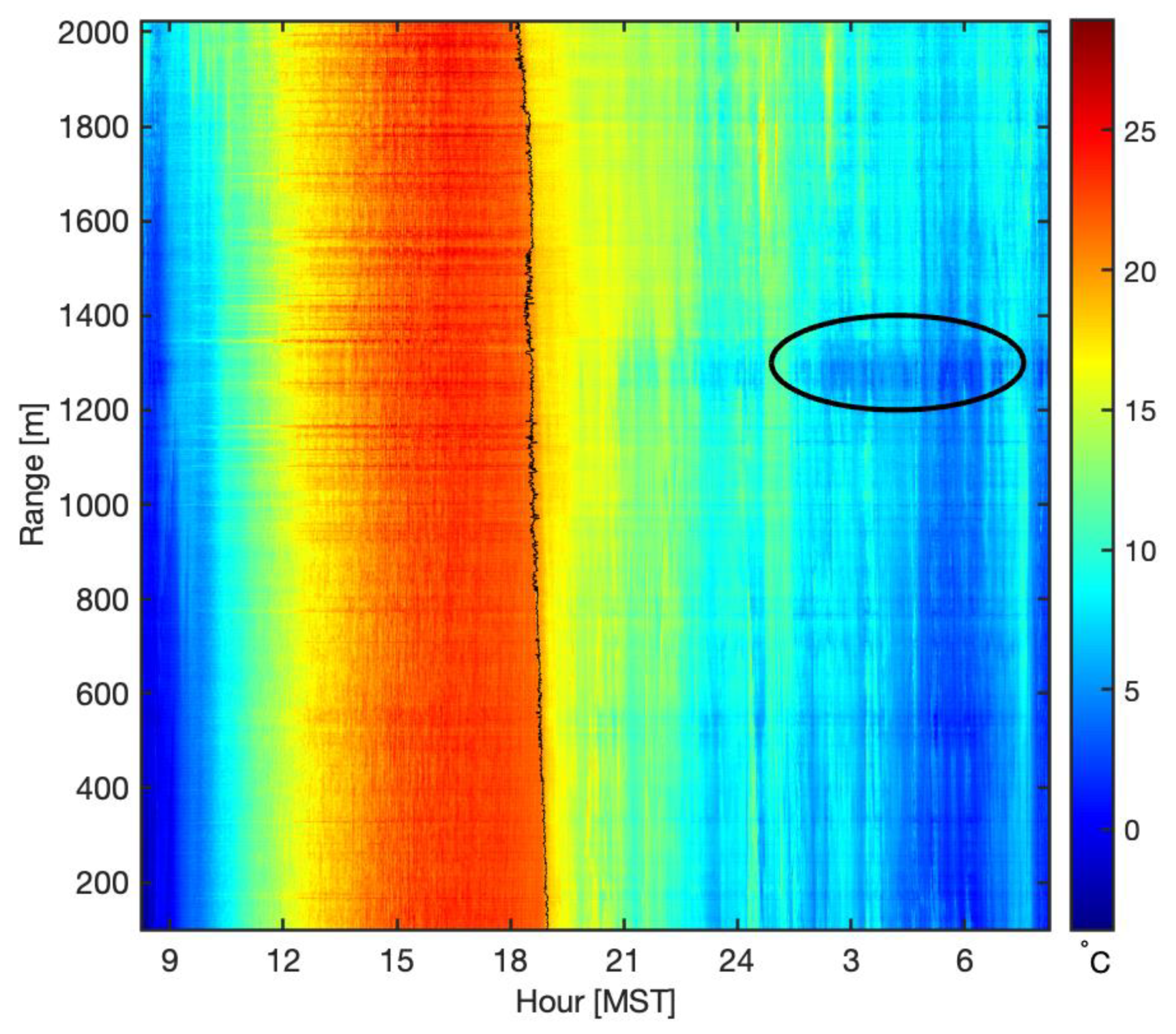
3.1.2. Diurnal Evolution of Near-Surface Temperature

Diurnal evolution of the near surface (0.5 m) temperature field along the DTS deployment is shown in Figure 5 for 8–9 October. On the east side of Granite Peak, higher elevations were shaded before lower elevations as the sun dipped below the ridgeline, delineated by the thin black line in Figure 5. This feature was called the “shade front” in [11,22,31] and the “transition front” in [40]. In this paper, we refer to the transition between daylight and shade as the shade front. Maximum curvature in the temperature gradient was used to define the shade front in Figure 5 and subsequent analyses. The tilt of the black line is consistent with a shade front propagating downslope (as expected for an easterly aspect). After the shade front passed, radiative cooling at higher elevations preceded lower-level cooling and initiated downslope flow. Intermittent entrainment of warm air at high elevations constrained cooling as cold air intensified at lower elevations due to both longwave cooling and cold air pooling. These features are consistent with textbook cold air drainage flow [41]. Not so textbook are the subtle vertical and horizontal banded features in the temperature trace. The vertical bands after the shade front passes are large temperature fluctuations (LTF’s −3 °C or greater temperature drops in a 30-min period) or oscillations that [42] identified and associated with cold-air pool displacements. The horizontal bands are not image production artefacts, but rather are signatures of small-scale drainage channels. For example, the region enclosed by an ellipse in Figure 5 corresponds to a large gulley at an approximately 1300-m range in Figure 6b. In Figure 6 and subsequent plots, daytime averages are computed from the noon to 1 PM MST time frame and nighttime averages are computed between midnight and 1 AM MST.

3.2. Lapse Rate Scale Dependencies

3.2.1. Dependency of Near-Surface Lapse Rate to Flow Channel Proximity

Average daytime temperature along the fiber is plotted at the two fiber heights (0.5 m and 1.0 m) in Figure 6a and during the nighttime in Figure 6b. For both panels in Figure 6b, vertical shading demarks the horizontal extent of drainage features, as determined from GPS measurements (see also Figure 2). Daytime warm air at 0.5 m at 100-m range transitions to well-mixed air at approximately 1100-m ranges, as indicated by the convergence of the 0.5- and 1.0-m temperature traces. At nighttime (Figure 6b), the DTS data indicate statically stable conditions everywhere along the transect with cold air anomalies occupying the drainage channels regardless of channel cross-sectional diameter. During the daytime (Figure 6a), there is less correspondence between the drainage channel position and temperature. As indicated by the daytime hatching patterns in Figure 5, solar heating also impacts air temperature within small-scale flow channels during the day, but the impact depends on solar aspect that varies across the channel cross-section. During the night, cold air fills gullies that preferentially channel the coldest air.

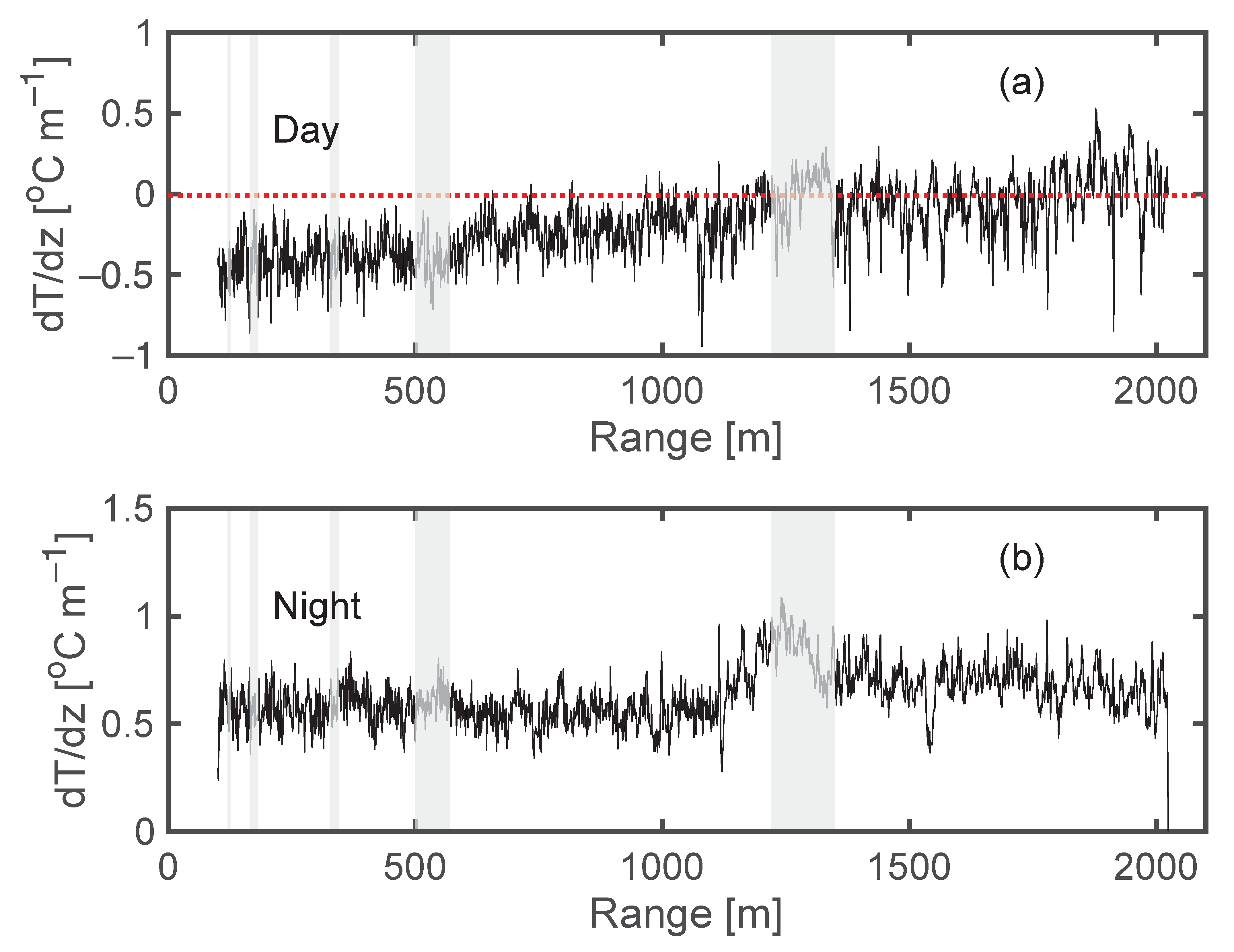
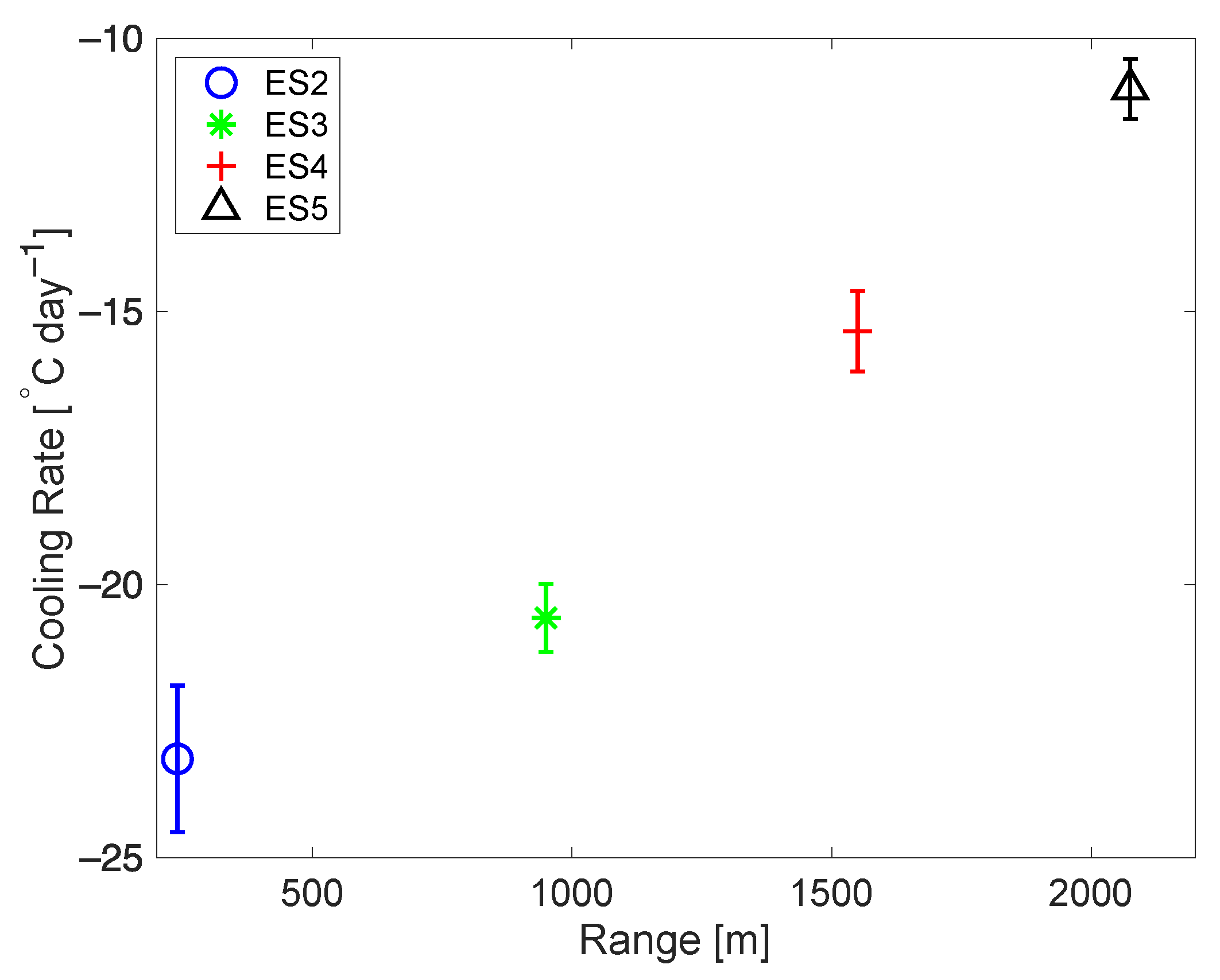
3.2.2. Dependency of Near-Surface Lapse Rate to Downslope Distance (Range)

At the local scale, Figure 6 shows that the position relative to nearby drainage channels highly correlates with air temperature throughout the night, but to a lesser extent throughout the day. To what degree does distance down the slope influence local temperature gradients? In Figure 7, the near-surface lapse rate is plotted as a function of distance along the DTS transect. The vertical temperature gradient is computed from the difference between 0.5-m and 1.0-m height temperatures during the day (panel a) and night (panel b). The daytime lapse rate along the DTS transect shown in Figure 7a indicates that lapse rate decreases in absolute magnitude from superadiabatic at low elevations to adiabatic, although with greater variability, at higher elevations. For reference, the dry adiabatic lapse rate (−0.0098 °C m−1) is rendered as a dotted red line in Figure 7a. The lapse rate is stable along the DTS transect (Figure 7b) and indicates that range has little influence on the local nocturnal lapse rate.

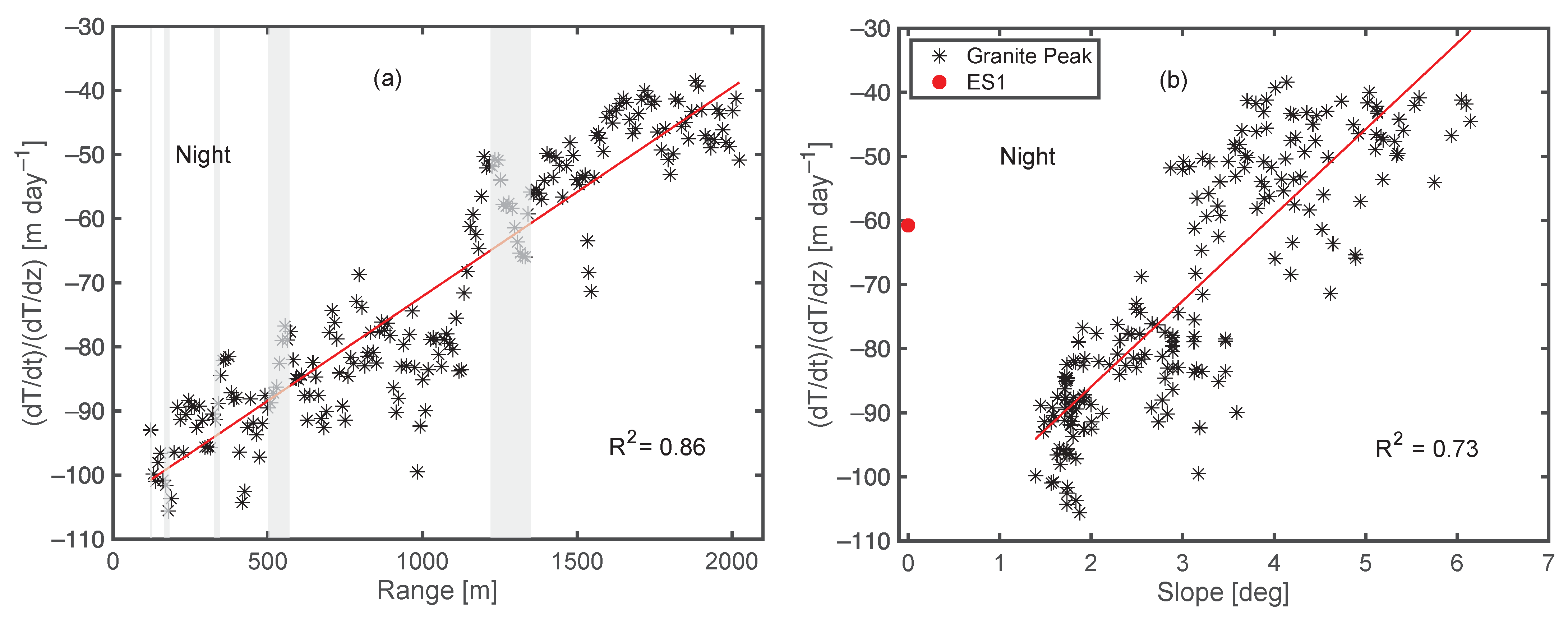
3.3. Cooling Rate Scale Dependencies

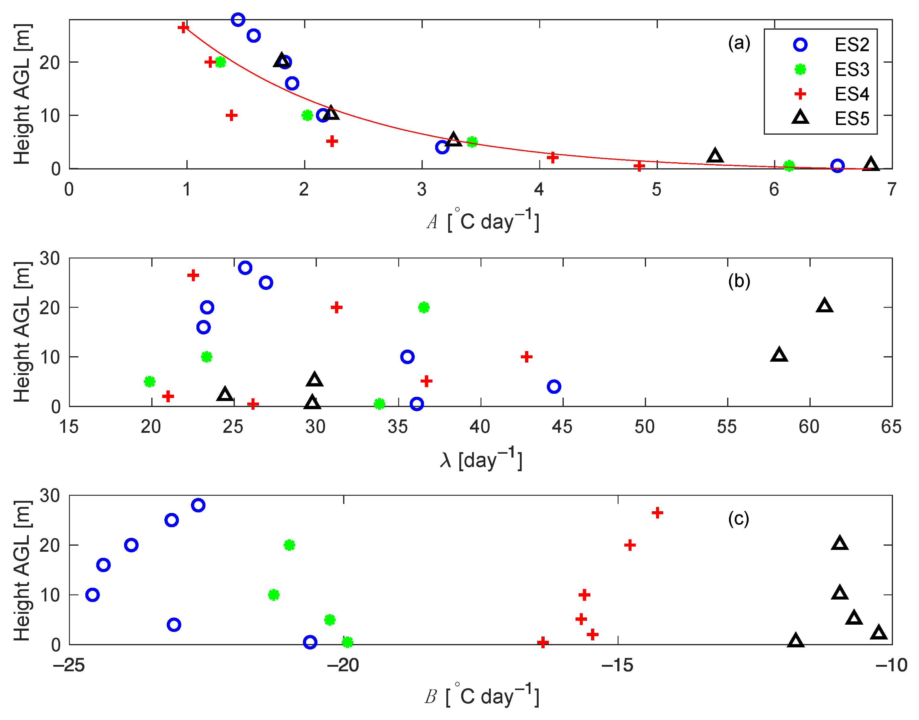
3.3.1. Dependency of Cooling Rate to Height and Day/Night Transition

Vertical temperature profiles from tower data are used to resolve cooling rate through a deeper layer than measured with the DTS. For 24-h periods spanning 8–9, 9–10, and 13–14 October, the ensemble averaged temperature field at five heights on tower ES5 are plotted in Figure 8a. In Figure 8a, solar insolation produces higher temperatures near the ground as the day progresses. After the sun is eclipsed by the Granite Peak ridgeline at approximately 16:25 MST, the lowest levels (0.55 m and 2.14 m) cool more rapidly than higher levels, producing a near-surface temperature inversion.
Between 5.1 m and 20 m at tower ES5 (panel a), a well-mixed residual layer persists with air temperature that is approximately isothermal, consistent with relatively uniform R i B above a 10-m height in Figure 4e. A faster cooling rate, given by the larger negative slope of the temperature traces, is evident further downslope at tower ES2 (Figure 8b), relative to ES5. By inspection, the localized transition from day to night exhibits a decay in temperature that approximates exponential decay at both ES2 and ES5. Subsequently, air temperature transitions to a more linear decrease with time. This trend was observed at all five towers. Unlike results in [43] (Figure 3), the vertical temperature profile changes with time. Figure 6 and Figure 7 in [22] document similar decay in temperature after the shade front passed over a tower on a steep slope in the Swiss Alps. Others have noted a shading-induced temperature decay feature in different environments, including over a glacier [44], near an airport in Nepal [9], and in an incised watershed in the Oregon Cascades [45].
DTS measurements along the fiber revealed a similar exponential decay in temperature with time after a given fiber segment was topographically shaded. Ignoring mixing-induced temperature variations, characteristic curves following the shade front passage suggest a mathematical expression of the form:
d T d t = A e λ t + B t ,
where A and B are constants, t is time after shade front passage, and λ is a decay constant.

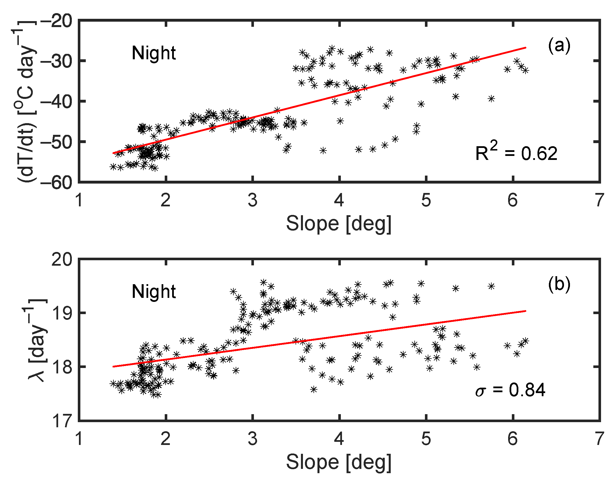
3.3.2. Dependency of Cooling Rate to Slope Angle

DTS data provide fewer vertical levels but finer grained along-slope representation of local cooling rate than the tower data. During a one-hour nighttime period (0000 to 0100 MST) on 8–9 October, Figure 9a shows that local cooling rate increases with slope as predicted by [46]. For our data set, the correlation between slope and cooling rate decreased as the slope increased above 3°. Transverse and longitudinal instability modes possibly influenced the observed variability in cooling rate although longitudinal modes are consequential at higher slope angle and transverse mode instability decreases with increasing slope angle [47]. As shown in Figure 2, steeper slopes were also rougher so topographic variability likely increased variability in the cooling rate. For the same time period and at the same positions as in Figure 9a, the value of λ from Equation (2) is nearly constant as the slope increases, as shown in Figure 9b. One extraneous point with a value of λ = 9.7 lies beyond the plotting boundary in Figure 9b. The average decay “constant” of 18.5 day−1 is less than the value found from tower data. This topic is revisited in the discussion section.

3.3.3. Basin-Scale Cooling Rate

The DTS obtains high spatial resolution temperature data over several kilometers so one can examine the influence that range has on basin-scale cooling rate. Upon the passage of the shade front, it was shown in Section 3.3.1 that the local lapse rate initially decreased exponentially with time and transitioned to a linear decrease. Local, nocturnal lapse rates were well correlated with position relative to topographic features (Figure 6b) but poorly correlated with downslope range (Figure 7b). To examine the basin-scale cooling rate, the local nocturnal cooling rate is divided by the local lapse rate and plotted as a function range (Figure 10a) and slope (Figure 10b). The units of the ordinate are in meters per day and represent the average rate of change in height of an isotherm at nighttime. Dividing the local cooling rate by the local lapse normalizes out variability in air temperature due to local lapse rate, yielding a function that serves as a proxy for basin-scale cooling rate, which we refer to as the basin-scale cooling proxy (BCP). Both plots in Figure 10 suggest linear relationships.
In Figure 10b, the measurement at the base of the slope (at ES1), several km east of ES2, indicates a different BCP regime relative to the towers on the slope. To summarize, at the onset of cooling, a position relative to topographic drainage features and local advection dominate the cooling rate, and we observe an exponential decay in near-surface air temperature, whilst at long timescales the large-scale drainage dominates, and the cooling rate scales linearly with slope and range.

4. Discussion

In this discussion, we refer to the first term on the r.h.s. of Equation (2) as the exponential decay term and the second term as the linear term. As shown in Figure 8 and Figure 9b, the exponential decay term agrees with the empirical result at local scales and was applicable after the shade front passed. Subsequently, the cooling rate at a given tower position was linear (Figure 8). Likewise, when the cooling rate at each DTS position was normalized by the local-scale lapse rate, the BCP was linear relative to both range and slope (Figure 10), corresponding to the linear limiting case in Equation (2). Three measures of position were examined—slope, range, and position relative to drainage features, and the influence of these parameters is scale-dependent. Equation (2) serves as an objective measure of the range of influence for cooling rate. We acknowledge a deficiency that the linear term lacks a representation for the time delay between buoyancy forcing as surface air cools and when drainage flow dynamically responds, which could be addressed in future studies.
Using tower data, the magnitudes of coefficients in Equation (2) were calculated and plotted in Figure 11. Parameters A , λ , and B are plotted in panels a, b, and c, respectively, for towers along the DTS transect. The time span for the exponential decay in Figure 8 was chosen to optimize the fit to the large magnitude slope change during the initial decay period and minimize the change in slope in the transition between the period of exponentially decreasing temperature and the linear temperature decrease period. This methodology yielded an 1 2 3 h period for exponential decay. By comparison, [11] noted a 2-h period of exponential decay based on MATERHORN tower data. For a steeper, smaller drainage near La Fouly, Switzerland, [22] found exponential decay in the temperature field for a 1.5-h period. Following the passage of the shade front, there was a ~10-min transition period (which was height dependent) before an inflection point at which time temperature began to decrease exponentially and the 1 2 3 h period of exponentially decreasing temperature does not include this transition period, which would partially account for the 20-min discrepancy between our result and that of [11].
The curve fit (red line in Figure 11a) of the A parameter in Equation (2) has form: A ( z ) = a + b e c z with coefficients: a = −0.672, b = 52.102, c = 0.662. Figure 11b shows that the λ parameter in Equation (2) had a larger mean and greater variability than that found for DTS data (Figure 9b), ranging from 20 to 60 with a 32 ± 11 day−1 mean. Note that the decay constant λ is the inverse of a time constant. It is not surprising that the temperature time constant of air not close to the surface and not located in a gulley is more variable and relatively more responsive to processes other than surface cooling. Parameter B , plotted in Figure 11c, has values clustered in order, according to downslope range. That is, the highest elevation station, ES5 had the lowest value of B in absolute magnitude and station ES2 had the highest value for B in absolute magnitude. Comparing the mean of B at each station as a function of downslope range yielded an equation for B as a function of range: B ( x ) = m x + b with coefficients: m: 0.00681 and b: −25.72.
Figure 12 shows the composited, mean cooling rate as a function of range during the time period of 110 min after the shade front passage and the next 10 h thereafter, as measured at towers ES2 through ES5. Unlike the linear cooling rate with range found for DTS data in Figure 10a, the cooling rate vs. range for the tower data is not quite linear, exhibiting weak exponential decay from high elevations to low elevations. The local contribution to cooling rate was normalized out of Figure 10, whereas the tower data in Figure 12 contain multi-scale contributions, from local to basin-wide. We attribute the non-linearity evident in Figure 12 to the local-scale contribution expressed in the larger scale cooling rate.

5. Conclusions

DTS and tower-based instrumentation were deployed to examine the influence of spatial scale on drainage cooling rate, which is correlated with katabatic wind speed. The DTS provided temperature gradient measurements of the 0.5–1-m air layer at an unprecedented combination of spatial and temporal scales, enabling multiscalar examination of katabatic flow development. Shortly after the evening arrival of the shade front, the local cooling rate reached a maximum value, decayed exponentially, and then transitioned to a linear cooling rate with time. For this experiment, the decay constant for the 0.5–1-m layer was 18.5 dy−1 and the magnitude and variability of the decay constant increased with height. The basin-scale cooling rate was linear with both slope and range. An empirically derived function (Equation (2)) describes the evolution of the near-surface temperature field due to local-to-basin scale influences. Subsequent to shade front passage, local cooling rate evolution was not monotonic, in part, because of the intermittent influence of meandering downslope velocity maxima.
Whereas many previous experiments have primarily focused on the vertical wind speed profile of katabatic flow [4,13,44,48,49], a novel aspect of this study is to address the role that measures of spatial scale have for katabatic flow development. To the authors’ knowledge, multiscale analysis of the near-surface katabatic temperature field ranging from the submeter scale to the kilometer scale has not previously been performed. Scale specific results include:
  • At local scales, the critical length scale is position relative to a local drainage feature. It is likely that advection through these local features account for a disproportionate amount of the total transport (the timescales are faster) but local-scale flux measurements to verify this hypothesis were unavailable during the MATERHORN experiment;
  • With increasing spatial and temporal scale, slope and range become the most important causative spatial variables;
  • Katabatic wind speed at a given location downrange is therefore an integration of local and basin scale contributions, both of which evolve in magnitude following shade front passage.
Neither Prandtl’s equation for drainage flow nor model simulations resolve the effect of timescale variability due to small-scale topographic features. Since the variability in timescales increases with terrain complexity, studies with underlying idealized topography do not capture the effect that multiple scales of topography have on drainage flow time scales. These results indicate that partitioning between scales of influence can provide novel insights into the evolution of drainage flow.

Author Contributions

Conceptualization and methodology: C.H.; software, validation, formal analysis, investigation, resources: C.H. and S.D.; data curation: E.P. and C.H.; writing—original draft preparation, S.D.; writing—review and editing: C.H., E.P. and S.D.; visualization: C.H. and S.D.; funding acquisition: C.H. and E.P. All authors have read and agreed to the published version of the manuscript.

Funding

This research was funded in part through a National Science Foundation, award EAR-1440506, to the Center for Transformative Environmental Monitoring Programs (CTEMPs). This research was funded in part by the Office of Naval Research Award N00014-11-1-0709, Mountain Terrain Atmospheric Modeling and Observations (MATERHORN) Program. The APC was funded by the Department of Physics, University of Nevada, Reno.

Institutional Review Board Statement

Not applicable.

Informed Consent Statement

Not applicable.

Data Availability Statement

Tower data are available in Matlab format from E.P. Synthesized DTS data are available in Matlab format from C.H.

Acknowledgments

We thank Derek Jensen for acquiring and sharing the meteorological tower data referenced in this manuscript. The authors gratefully acknowledge two anonymous reviewers for their suggestions to improve this manuscript.

Conflicts of Interest

The authors declare no conflict of interest. The funders had no role in the design of the study; in the collection, analyses, or interpretation of data; in the writing of the manuscript, or in the decision to publish the results.

References

  1. Papadopoulos, K.H.; Helmis, C.G.; Soilemes, A.T.; Kalogiros, J.; Papageorgas, P.G.; Asimakopoulos, D.N. The structure of katabatic flows down a simple slope. Q. J. R. Meteorol. Soc. 1977, 123, 1581–1601. [Google Scholar] [CrossRef]
  2. Kondo, J.; Sato, T. A simple model of drainage flow on a slope. Bound.-Layer Meteorol. 1988, 43, 103–123. [Google Scholar] [CrossRef]
  3. Barr, S.; Kyle, T.G.; Clements, W.E.; Sedlacek, W. Plume dispersion in a nocturnal drainage wind. Atmos. Environ. 1983, 17, 1423–1429. [Google Scholar] [CrossRef]
  4. Yasuda, N.; Kondo, J.; Sato, T. Drainage flow observed in a V-shaped valley. J. Meteorol. Soc. Jpn. Ser. II 1986, 64, 283–301. [Google Scholar] [CrossRef] [Green Version]
  5. Wilson, J.G.; Kingham, S.; Sturman, A.P. Intraurban variations of PM10 air pollution in Christchurch, New Zealand: Implications for epidemiological studies. Sci. Total Environ. 2006, 367, 559–572. [Google Scholar] [CrossRef]
  6. Bale, J.S.; Harrington, R.; Clough, M.S. Low temperature mortality of the peach-potato aphid Myzus persicae. Ecol. Entomol. 1988, 13, 121–129. [Google Scholar] [CrossRef]
  7. Lindkvist, L.; Chen, D. Air and soil frost indices in relation to plant mortality in elevated clear-felled terrain in Central Sweden. Clim. Res. 1999, 12, 65–75. [Google Scholar] [CrossRef] [Green Version]
  8. Darby, L.S.; Poulos, G.S. The evolution of lee-wave–rotor activity in the lee of Pike’s Peak under the influence of a cold frontal passage: Implications for aircraft safety. Mon. Weather Rev. 2006, 134, 2857–2876. [Google Scholar] [CrossRef] [Green Version]
  9. Regmi, R.P. Aviation hazards over the Jomsom Airport of Nepal as revealed by numerical simulation of local flows. J. Inst. Sci. Technol. 2015, 19, 111–120. [Google Scholar] [CrossRef] [Green Version]
  10. Hang, C.; Nadeau, D.F.; Gultepe, I.; Hoch, S.W.; Román-Cascón, C.; Pryor, K.; Fernando, H.J.S.; Creegan, E.D.; Leo, L.S.; Silver, Z.; et al. A Case Study of the Mechanisms Modulating the Evolution of Valley Fog. Pure Appl. Geophys. 2016, 173, 3011–3030. [Google Scholar] [CrossRef]
  11. Jensen, D.D.; Nadeau, D.F.; Hoch, S.W.; Pardyjak, E.R. The evolution and sensitivity of katabatic flow dynamics to external influences through the evening transition. Q. J. R. Meteorol. Soc. 2017, 143, 423–438. [Google Scholar] [CrossRef]
  12. Poulos, G.; Zhong, S. An observational history of small-scale katabatic winds in mid-latitudes. Geogr. Compass 2008, 2, 1798–1821. [Google Scholar] [CrossRef]
  13. Yi, C.; Monson, R.K.; Zhai, Z.; Anderson, D.E.; Lamb, B.; Allwine, G.; Turnipseed, A.A.; Burns, S.P. Modeling and measuring the nocturnal drainage flow in a high-elevation, subalpine forest with complex terrain. J. Geophys. Res.-Atmos. 2005, 110. [Google Scholar] [CrossRef] [Green Version]
  14. Mahrt, L. Momentum balance of gravity flows. J. Atmos. Sci. 1982, 39, 2701–2711. [Google Scholar] [CrossRef] [Green Version]
  15. Garrett, A.J. Drainage flow prediction with a one-dimensional model including canopy, soil and radiation parameterizations. J. Clim. Appl. Meteorol. 1983, 22, 79–91. [Google Scholar] [CrossRef] [Green Version]
  16. McCumber, M.C.; Pielke, R.A. Simulation of the effects of surface fluxes of heat and moisture in a mesoscale numerical model: 1. Soil layer. J. Geophys. Res.-Oceans 1981, 86, 9929–9938. [Google Scholar] [CrossRef] [Green Version]
  17. Ookouchi, Y.; Segal, M.; Kessler, R.C.; Pielke, R.A. Evaluation of soil moisture effects on the generation and modification of mesoscale circulations. Mon. Weather Rev. 1984, 112, 2281–2292. [Google Scholar] [CrossRef] [Green Version]
  18. Skyllingstad, E.D. Large-eddy simulation of katabatic flows. Bound.-Layer Meteorol. 2003, 106, 217–243. [Google Scholar] [CrossRef]
  19. de Bode, M.; Hedde, T.; Roubin, P.; Durand, P. Fine-Resolution WRF Simulation of Stably Stratified Flows in Shallow Pre-Alpine Valleys: A Case Study of the KASCADE-2017 Campaign. Atmosphere 2021, 12, 1063. [Google Scholar] [CrossRef]
  20. Selker, J.; van de Giesen, N.; Westhoff, M.; Luxemburg, W.; Parlange, M.B. Fiber optics opens window on stream dynamics. Geophys. Res. Lett. 2006, 33. [Google Scholar] [CrossRef] [Green Version]
  21. Fernando, H.J.S.; Pardyjak, E.R.; Di Sabatino, S.; Chow, F.K.; De Wekker, S.F.J.; Hoch, S.W.; Hacker, J.; Pace, J.C.; Pratt, T.; Pu, Z.; et al. The MATERHORN: Unraveling the intricacies of mountain weather. Bull. Am. Meteorol. Soc. 2015, 96, 1945–1967. [Google Scholar] [CrossRef]
  22. Nadeau, D.F.; Pardyjak, E.R.; Higgins, C.W.; Huwald, H.; Parlange, M.B. Flow during the evening transition over steep Alpine slopes. Q. J. R. Meteorol. Soc. 2013, 139, 607–624. [Google Scholar] [CrossRef]
  23. Selker, J.S.; Thévenaz, L.; Huwald, H.; Mallet, A.; Luxemburg, W.; Van De Giesen, N.; Stejskal, M.; Zeman, J.; Westhoff, M.; Parlange, M.B. Distributed fiber-optic temperature sensing for hydrologic systems. Water Resour. Res. 2006, 42. [Google Scholar] [CrossRef] [Green Version]
  24. Tyler, S.W.; Selker, J.S.; Hausner, M.B.; Hatch, C.E.; Torgersen, T.; Thodal, C.E.; Schladow, S.G. Environmental temperature sensing using Raman spectra DTS fiber-optic methods. Water Resour. Res. 2009, 45. [Google Scholar] [CrossRef] [Green Version]
  25. Sayde, C.; Buelga, J.B.; Rodriguez-Sinobas, L.; El Khoury, L.; English, M.; van de Giesen, N.; Selker, J.S. Mapping variability of soil water content and flux across 1–1000 m scales using the Actively Heated Fiber Optic method. Water Resour. Res. 2014, 50, 7302–7317. [Google Scholar] [CrossRef] [Green Version]
  26. Bense, V.F.; Read, T.; Verhoef, A. Using distributed temperature sensing to monitor field scale dynamics of ground surface temperature and related substrate heat flux. Agric. Forest Meteorol. 2016, 220, 207–215. [Google Scholar] [CrossRef] [Green Version]
  27. Thomas, C.K.; Kennedy, A.M.; Selker, J.S.; Moretti, A.; Schroth, M.H.; Smoot, A.R.; Tufillaro, N.B.; Zeeman, M.J. High-resolution fibre-optic temperature sensing: A new tool to study the two-dimensional structure of atmospheric surface-layer flow. Bound.-Layer Meteorol. 2012, 142, 177–192. [Google Scholar] [CrossRef]
  28. Sayde, C.; Thomas, C.K.; Wagner, J.; Selker, J.S. High-resolution wind speed measurements using actively heated fiber optics. Geophys. Res. Lett. 2015, 42, 10–064. [Google Scholar] [CrossRef] [Green Version]
  29. Higgins, C.W.; Wing, M.G.; Kelley, J.; Sayde, C.; Burnett, J.; Holmes, H.A. A high resolution measurement of the morning ABL transition using distributed temperature sensing and an unmanned aircraft system. Environ. Fluid Mech. 2018, 18, 683–693. [Google Scholar] [CrossRef]
  30. Van De Giesen, N.; Steele-Dunne, S.C.; Jansen, J.; Hoes, O.; Hausner, M.B.; Tyler, S.; Selker, J. Double-ended calibration of fiber-optic Raman spectra distributed temperature sensing data. Sensors 2012, 12, 5471–5485. [Google Scholar] [CrossRef] [Green Version]
  31. Lehner, M.; Whiteman, C.D.; Hoch, S.W.; Jensen, D.; Pardyjak, E.R. A case study of the nocturnal boundary-layer evolution on a slope at the foot of a desert mountain. J. Appl. Meteorol. Climatol. 2015, 54, 732–751. [Google Scholar] [CrossRef]
  32. Smith, F.B.; Abbott, P.F. Statistics of lateral gustiness at 16 m above ground. Q. J. R. Meteorol. Soc. 1961, 87, 549–561. [Google Scholar] [CrossRef]
  33. Hanna, S.R. Lateral turbulence intensity and plume meandering during stable conditions. J. Clim. Appl. Meteorol. 1983, 22, 1424–1430. [Google Scholar] [CrossRef] [Green Version]
  34. Drake, S.A.; McKay, L.; Abernathy, R.N.; Skupniewicz, C.E.; Kamada, R.F. Lompoc Valley Diffusion Experiment Data Report; Tech Rep No. NPS-PH-91-001; PN: Naval Postgraduate School Monterey: Monterey, CA, USA, 1990. [Google Scholar]
  35. Kurzeja, R.J.; Berman, S.; Weber, A.H. A climatological study of the nocturnal planetary boundary layer. Bound.-Layer Meteorol. 1991, 54, 105–128. [Google Scholar] [CrossRef]
  36. Monti, P.; Fernando, H.J.S.; Princevac, M.; Chan, W.C.; Kowalewski, T.A.; Pardyjak, E.R. Observations of flow and turbulence in the nocturnal boundary layer over a slope. J. Atmos. Sci. 2002, 59, 2513–2534. [Google Scholar] [CrossRef]
  37. Stull, R.B. An Introduction to Boundary Layer Meteorology; Springer: Berlin/Heidelberg, Germany, 2012; Volume 13. [Google Scholar]
  38. Grachev, A.A.; Leo, L.S.; Di Sabatino, S.; Fernando, H.J.S.; Pardyjak, E.R.; Fairall, C.W. Structure of turbulence in katabatic flows below and above the wind-speed maximum. Bound.-Layer Meteorol. 2016, 159, 469–494. [Google Scholar] [CrossRef] [Green Version]
  39. Mahrt, L.; Larsen, S. Relation of slope winds to the ambient flow over gentle terrain. Bound.-Layer Meteorol. 1990, 53, 93–102. [Google Scholar] [CrossRef]
  40. Hunt, J.C.R.; Fernando, H.J.S.; Princevac, M. Unsteady thermally driven flows on gentle slopes. J. Atmos. Sci. 2003, 60, 2169–2182. [Google Scholar] [CrossRef]
  41. Clements, C.B.; Whiteman, C.D.; Horel, J.D. Cold-air-pool structure and evolution in a mountain basin: Peter Sinks, Utah. J. Appl. Meteorol. 2003, 42, 752–768. [Google Scholar] [CrossRef]
  42. Jeglum, M.E.; Hoch, S.W.; Jensen, D.D.; Dimitrova, R.; Silver, Z. Large Temperature Fluctuations due to Cold-Air Pool Displacement along the Lee Slope of a Desert Mountain. J. Appl. Meteorol. Clim. 2017, 56, 1083–1098. [Google Scholar] [CrossRef]
  43. Horst, T.W.; Doran, J.C. Nocturnal drainage flow on simple slopes. Bound.-Layer Meteorol. 1986, 34, 263–286. [Google Scholar] [CrossRef]
  44. Oerlemans, J.; Grisogono, B. Glacier winds and parameterisation of the related surface heat fluxes. Tellus A 2002, 54, 440–452. [Google Scholar] [CrossRef]
  45. Pypker, T.G.; Hauck, M.; Sulzman, E.W.; Unsworth, M.H.; Mix, A.C.; Kayler, Z.; Bond, B.J. Toward using δ 13 C of ecosystem respiration to monitor canopy physiology in complex terrain. Oecologia 2008, 158, 399–410. [Google Scholar] [CrossRef]
  46. Fleagle, R.G. A theory of air drainage. J. Meteorol. 1950, 7, 227–232. [Google Scholar] [CrossRef] [Green Version]
  47. Xiao, C.N.; Senocak, I. Stability of the Prandtl model for katabatic slope flows. J. Fluid Mech. 2019, 865, R2. [Google Scholar] [CrossRef]
  48. Clements, W.E.; Archuleta, J.A.; Hoard, D.E. Mean structure of the nocturnal drainage flow in a deep valley. J. Appl. Meteorol. Clim. 1989, 28, 457–462. [Google Scholar] [CrossRef] [Green Version]
  49. Hootman, B.W.; Blumen, W. Analysis of nighttime drainage winds in Boulder, Colorado during 1980. Mon. Weather Rev. 1983, 111, 1052–1061. [Google Scholar] [CrossRef] [Green Version]
Figure 1. The DTS fiber transect extended from tower ES2 past tower ES5 on the SE side of Granite Peak. Drainage flow is from the WNW towards the ESE. Tower ES1 is on the playa east of ES2. (Figure contains modified Copernicus Sentinel data [2021] processed by Sentinel Hub).
Atmosphere 12 01651 g001
Figure 2. DTS transect with tower positions relative to elevation and slope.
Atmosphere 12 01651 g002
Figure 3. TKE time/height contours for tower ES4 for 7–14 October.
Atmosphere 12 01651 g003
Figure 4. For station ES4, wind direction in panel (a) shows 4-day composited downslope winds (westerly) at night and upslope (easterly) during the day. Composited temperature change at 0.5-m height plotted in 5-min intervals (panel (b)) shows that cooling rate is maximized after local sunset. The composited response in wind speed difference between 20 m and 2 m heights (panel (c)) occurs ~1–2 h after local sunset. Panel (d) shows a time/height contour plot of wind speed for the 8–9 October time period (not composited). Intermittent downslope wind speed maxima manifest at 5 m height during the night and deep upslope, insolation-driven wind speed maxima developed during the convective period. R i B for the time period in panel (d) are displayed in panel (e), showing development of a near-surface stable layer that deepens at night and erodes during the day.
Atmosphere 12 01651 g004
Figure 5. Space–time plot of temperature along the DTS fiber at a 0.5-m height during the night of 8–9 October. The thin black line delineates the sharp temperature gradient associated with the shade front propagating down the slope along the transect. Horizontal hatching is due to cold air drainage in small-scale gullies at night and preferential heating of the sunlit face of gullies during daytime. Hatching inside the oval region corresponds to a large gully evident at a 1300-m range in Figure 6b.
Atmosphere 12 01651 g005
Figure 6. Daytime (panel (a)) and nighttime (panel (b)) DTS temperature transects. At night, colder air occupies gullies. During the day surface temperature variability is greater and is less localized.
Atmosphere 12 01651 g006
Figure 7. Daytime (panel (a)) and nighttime (panel (b)) temperature lapse rate transects. At night, the local lapse rate is not a function of range.
Atmosphere 12 01651 g007
Figure 8. Ensemble temperature averages for 8–9, 9–10, and 13–14 October at ES5 (panel (a)) and ES2 (panel (b)). Grey regions indicate times that each station was shaded. In the absence of synoptic forcing, local temperature decays exponentially after the shade front passes the tower location.
Atmosphere 12 01651 g008
Figure 9. The correlation between dT/dt and slope (panel (a)) decreases at slope > 3 degrees. In panel (b), the decay “constant” λ in Equation (2) is nearly invariant with slope.
Atmosphere 12 01651 g009
Figure 10. Scatter plot showing the correlation between range and BCP (panel (a)). In panel (b), scatter plot showing the correlation between slope and BCP. This slope vs. BCP relationship is linearly correlated along the DTS transect and not correlated with the playa at tower ES1 (red dot).
Atmosphere 12 01651 g010
Figure 11. Panel (a) shows that the parameter A in Equation (2) is a function of height for the towers shown. The time constant, λ , (panel (b)) is variable over the range 20–45 with outliers up to ~60. Parameter B in Equation (2) is a function of downslope range (panel (c)).
Atmosphere 12 01651 g011
Figure 12. Cooling rate computed from tower-based air temperature.
Atmosphere 12 01651 g012
Publisher’s Note: MDPI stays neutral with regard to jurisdictional claims in published maps and institutional affiliations.

