
Probabilistic Inverse Method for Source Localization Applied to ETEX and the 2017 Case of Ru-106 including Analyses of Sensitivity to Measurement Data


Abstract
:1. Introduction
2. Materials and Methods
2.1. ETEX Dataset
2.2. Ru-106 Dataset
2.3. Meteorological Data
2.4. Dispersion Modelling
2.5. Source-Receptor Relationship
2.6. Proposed Method for Direct Marginal Posterior Estimation
2.6.1. Likelihood and Uncertainty Quantification
3. Results and Discussions
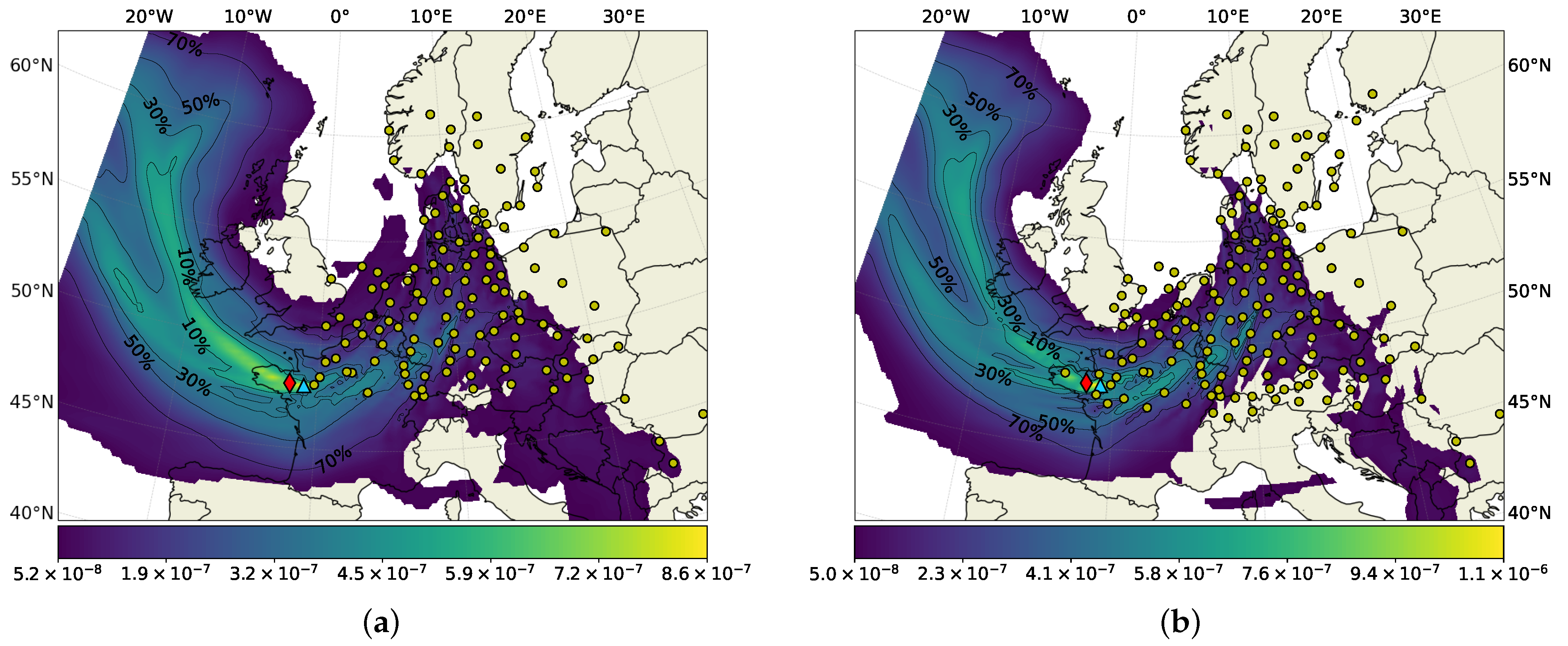
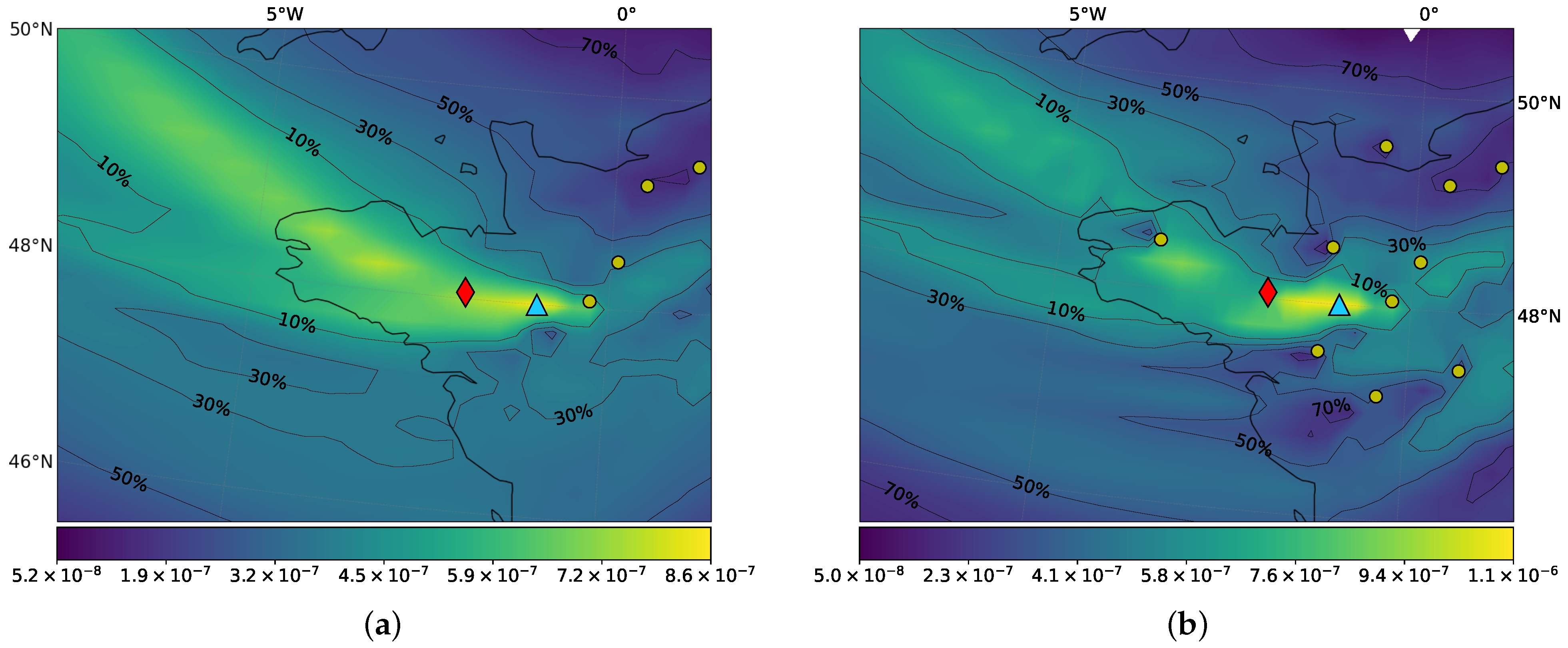
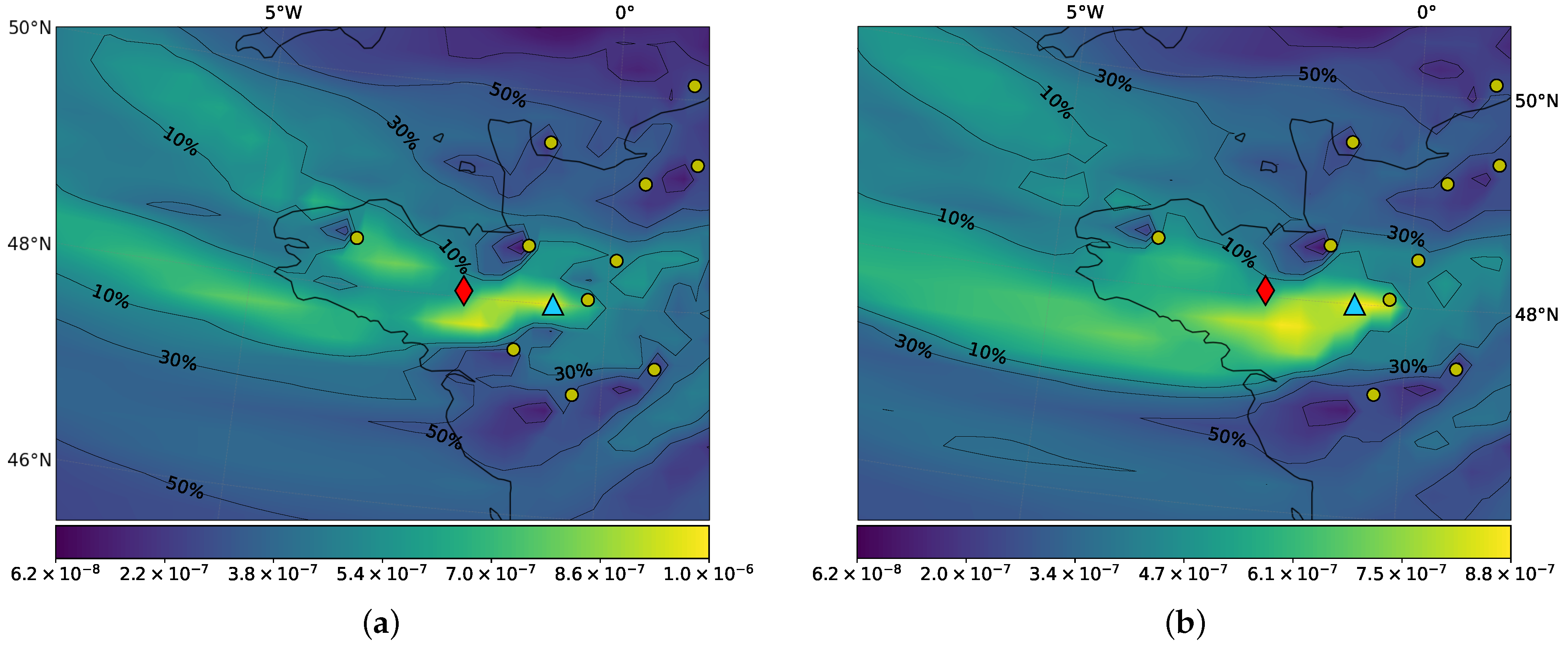
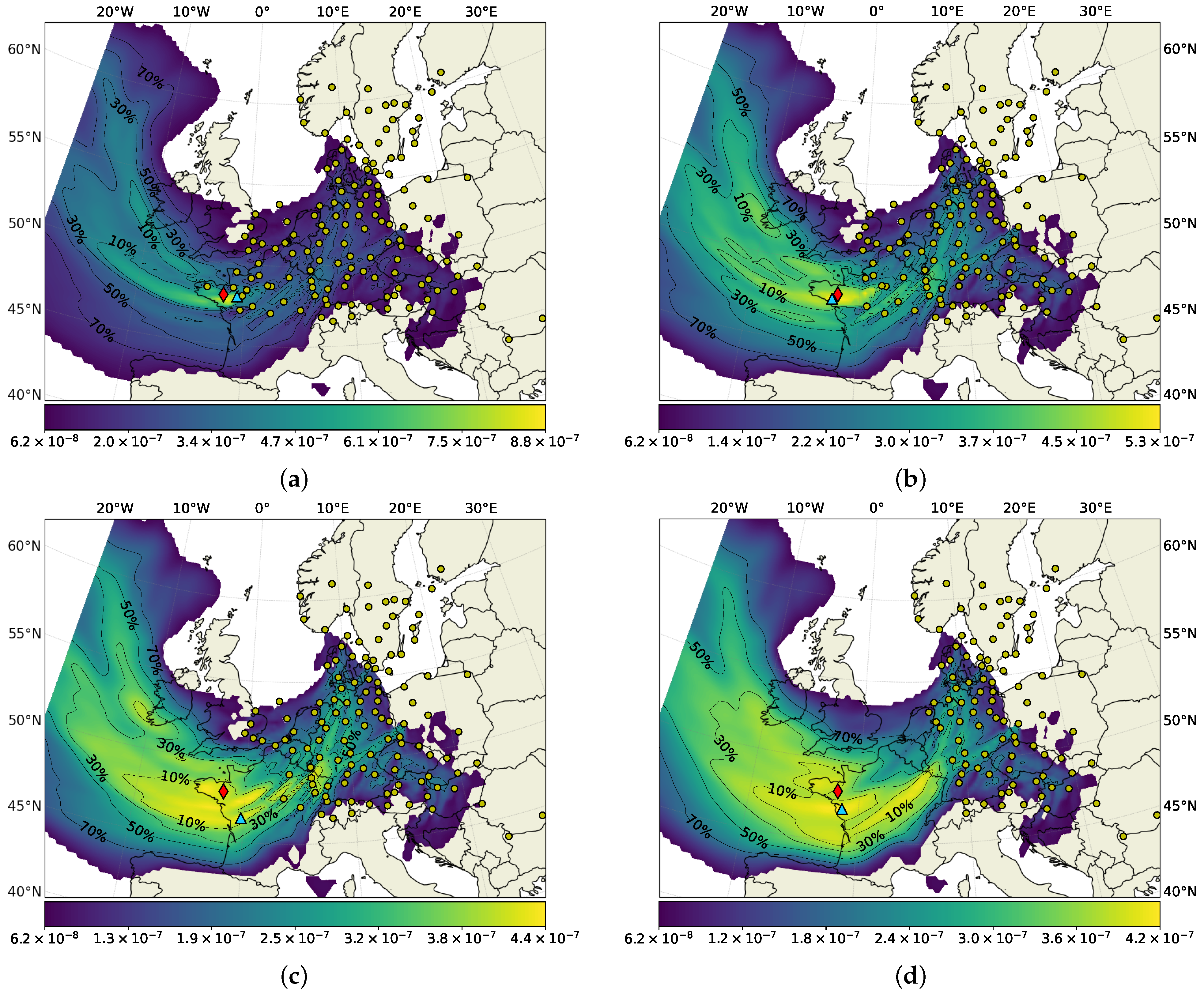
3.1. Application to the ETEX Case
3.1.1. Sensitivity Analyses
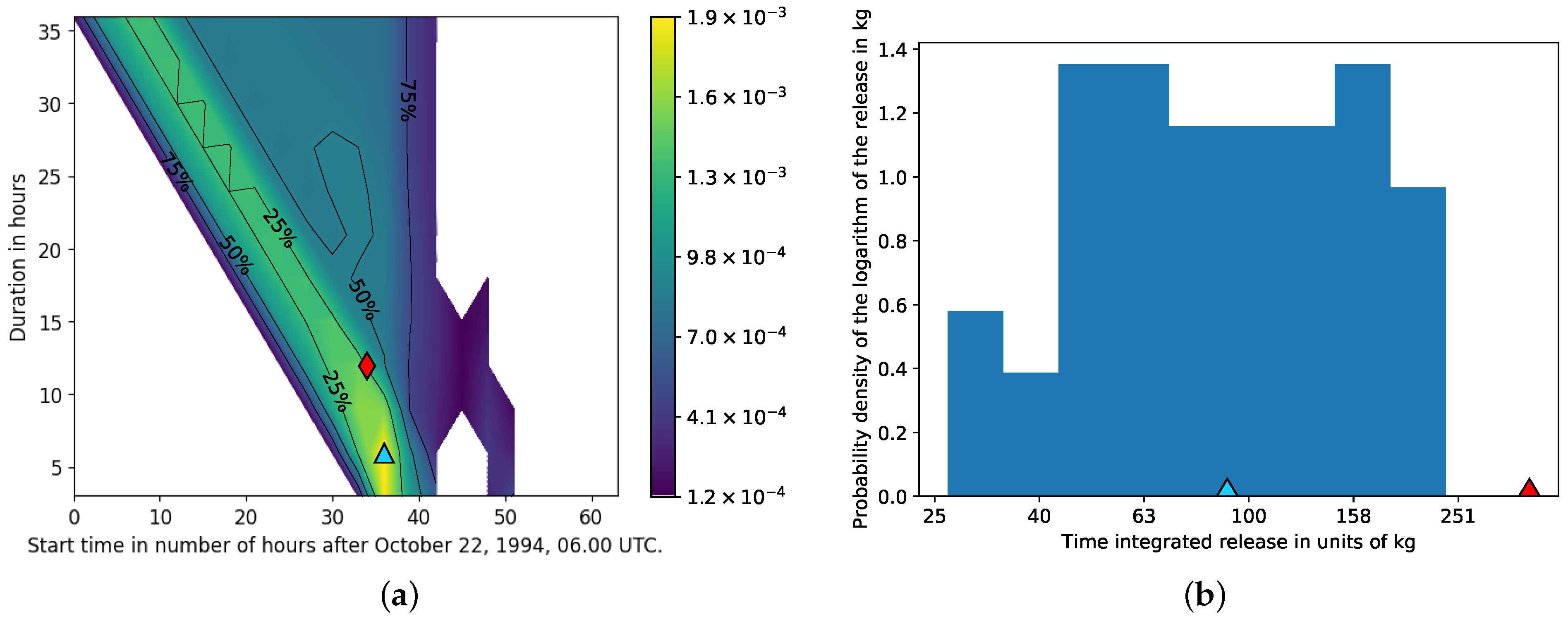
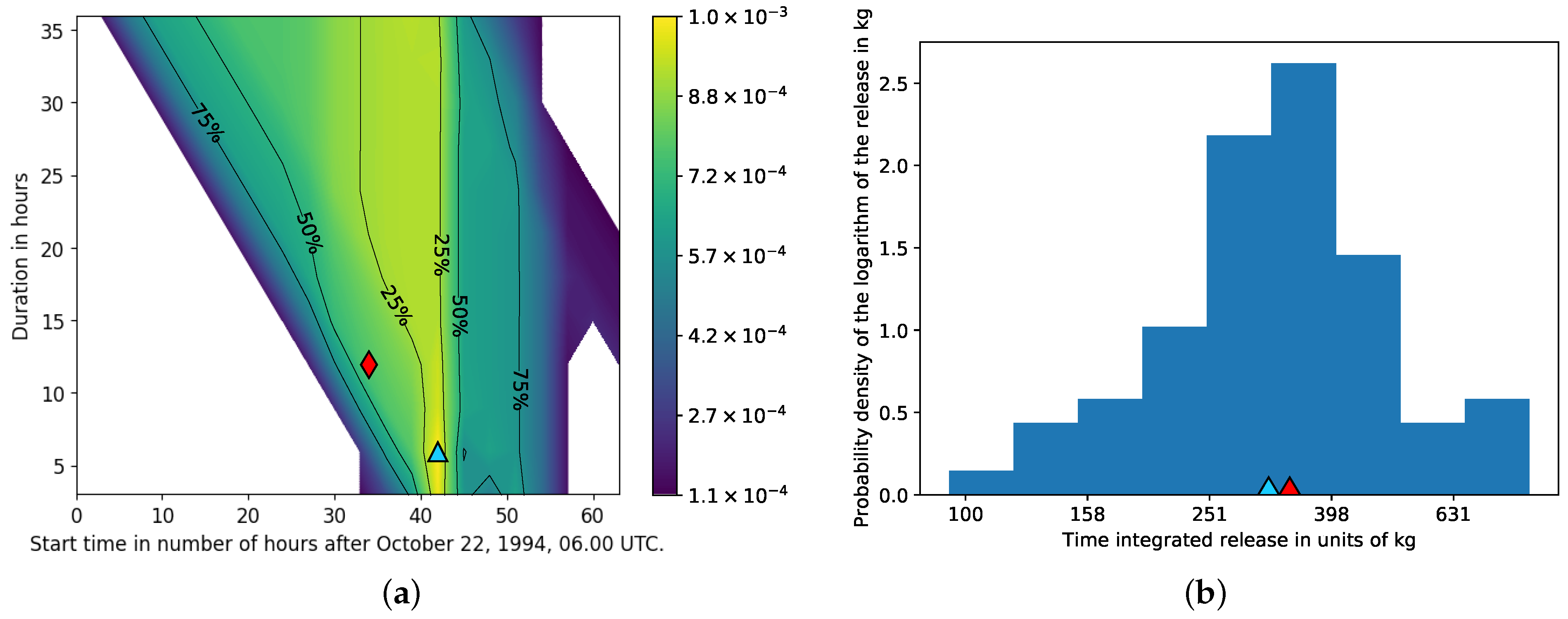
3.1.2. Time and Magnitude of the Release
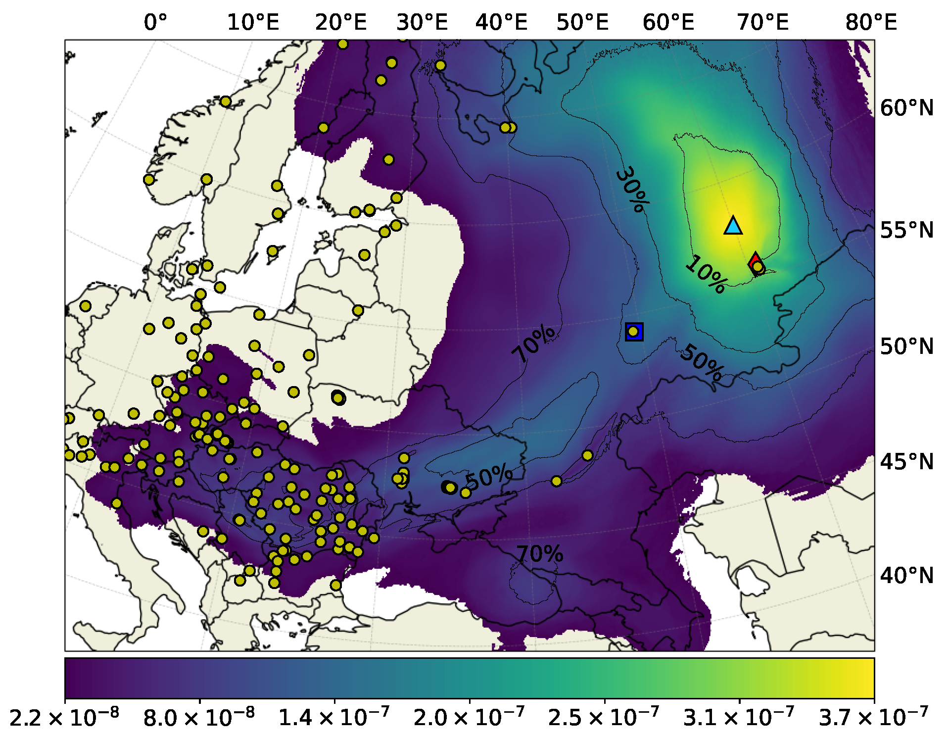
3.2. Application to the Ru-106 Case
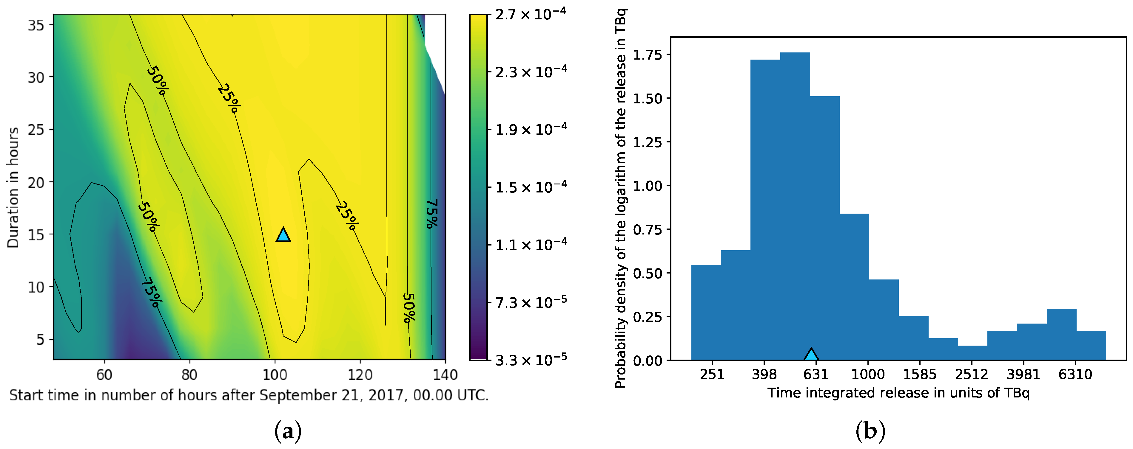
Time and Magnitude of the Release
4. Summary and Conclusions
Author Contributions
Funding
Institutional Review Board Statement
Informed Consent Statement
Data Availability Statement
Conflicts of Interest
Abbreviations
| DERMA | Danish Emergency Response Model of the Atmophere |
| PBL | Planetary Boundary Layer |
| ETEX | European Tracer Experiment |
| ECMWF | European Centre for Medium-Range Weather Forecasts |
| PMCH | Perfluoromethylcyclohexane |
| HDR | High Density Region |
References
- Pudykiewicz, J.A. Application of adjoint tracer transport equations for evaluating source parameters. Atmos. Environ. 1998, 32, 3039–3050. [Google Scholar] [CrossRef]
- Wotawa, G.; De Geer, L.E.; Denier, P.; Kalinowski, M.; Toivonen, H.; D’Amours, R.; Desiato, F.; Issartel, J.P.; Langer, M.; Seibert, P.; et al. Atmospheric transport modelling in support of CTBT verification—Overview and basic concepts. Atmos. Environ. 2003, 37, 2529–2537. [Google Scholar] [CrossRef]
- Seibert, P. Methods for source determination in the context of the CTBT radionuclide monitoring system. In Proceedings of the Informal Workshop on Meteorological Modelling in Support of CTBT Verification, Vienna, Austria, 4–6 December 2000; pp. 1–6. [Google Scholar]
- Seibert, P.; Frank, A.; Kromp-Kolb, H. Inverse modelling of atmospheric trace substances on the regional scale with Lagrangian models. In Proceedings of the EUROTRAC-2 Symposium, Garmisch-Partenkirchen, Germany, 11–15 March 2002; pp. 11–15. [Google Scholar]
- Sørensen, J.H. Method for source localization proposed and applied to the October 2017 case of atmospheric dispersion of Ru-106. J. Environ. Radioact. 2018, 189, 221–226. [Google Scholar] [CrossRef] [PubMed]
- Keats, A.; Yee, E.; Lien, F.S. Bayesian inference for source determination with applications to a complex urban environment. Atmos. Environ. 2007, 41, 465–479. [Google Scholar] [CrossRef]
- Yee, E.; Lien, F.S.; Keats, A.; D’Amours, R. Bayesian inversion of concentration data: Source reconstruction in the adjoint representation of atmospheric diffusion. J. Wind Eng. Ind. Aerodyn. 2008, 96, 1805–1816. [Google Scholar] [CrossRef]
- Yee, E.; Hoffman, I.; Ungar, K. Bayesian Inference for Source Reconstruction: A Real-World Application. Int. Sch. Res. Not. 2014, 2014, 12. [Google Scholar] [CrossRef] [Green Version]
- Saunier, O.; Didier, D.; Mathieu, A.; Masson, O.; Le Brazidec, J.D. Atmospheric modeling and source reconstruction of radioactive ruthenium from an undeclared major release in 2017. Proc. Natl. Acad. Sci. USA 2019, 116, 24991–25000. [Google Scholar] [CrossRef] [PubMed] [Green Version]
- Le Brazidec, J.D.; Bocquet, M.; Saunier, O.; Roustan, Y. MCMC methods applied to the reconstruction of the autumn 2017 Ruthenium-106 atmospheric contamination source. Atmos. Environ. X 2020, 6, 100071. [Google Scholar] [CrossRef]
- Efthimiou, G.C.; Kovalets, I.V.; Venetsanos, A.; Andronopoulos, S.; Argyropoulos, C.D.; Kakosimos, K. An optimized inverse modelling method for determining the location and strength of a point source releasing airborne material in urban environment. Atmos. Environ. 2017, 170, 118–129. [Google Scholar] [CrossRef]
- Kovalets, I.V.; Efthimiou, G.C.; Andronopoulos, S.; Venetsanos, A.G.; Argyropoulos, C.D.; Kakosimos, K.E. Inverse identification of unknown finite-duration air pollutant release from a point source in urban environment. Atmos. Environ. 2018, 181, 82–96. [Google Scholar] [CrossRef]
- Kovalets, I.V.; Romanenko, O.; Synkevych, R. Adaptation of the RODOS system for analysis of possible sources of Ru-106 detected in 2017. J. Environ. Radioact. 2020, 220, 106302. [Google Scholar] [CrossRef] [PubMed]
- Tomas, J.M.; Peereboom, V.; Kloosterman, A.; van Dijk, A. Detection of radioactivity of unknown origin: Protective actions based on inverse modelling. J. Environ. Radioact. 2021, 235, 106643. [Google Scholar] [CrossRef] [PubMed]
- Sørensen, J.H.; Klein, H.; Ulimoen, M.; Robertson, L.; Pehrsson, J.; Lauritzen, B.; Bohr, D.; Hac-Heimburg, A.; Israelson, C.; Buhr, A.M.B.; et al. NKS-430: Source Localization by Inverse Methods (SLIM); Technical Report; Nordic Nuclear Safety Research (NKS): Roskilde, Denmark, 2020. [Google Scholar]
- Graziani, G.; Klug, W.; Mosca, S. Real-Time Long-Range Dispersion Model Evaluation of the ETEX First Release; Office for Official Publications of the European Communities: Luxembourg, 1998. [Google Scholar]
- Nodop, K.; Connolly, R.; Girardi, F. The field campaigns of the European Tracer Experiment (ETEX): Overview and results. Atmos. Environ. 1998, 32, 4095–4108. [Google Scholar] [CrossRef]
- Masson, O.; Steinhauser, G.; Zok, D.; Saunier, O.; Angelov, H.; Babić, D.; Bečková, V.; Bieringer, J.; Bruggeman, M.; Burbidge, C.; et al. Airborne concentrations and chemical considerations of radioactive ruthenium from an undeclared major nuclear release in 2017. Proc. Natl. Acad. Sci. USA 2019, 116, 16750–16759. [Google Scholar] [CrossRef] [PubMed] [Green Version]
- Hersbach, H.; Bell, B.; Berrisford, P.; Hirahara, S.; Horányi, A.; Muñoz-Sabater, J.; Nicolas, J.; Peubey, C.; Radu, R.; Schepers, D.; et al. The ERA5 global reanalysis. Q. J. R. Meteorol. Soc. 2020, 146, 1999–2049. [Google Scholar] [CrossRef]
- PartIII: Dynamics and Numerical Procedures. In IFS Documentation CY47R1; IFS Documentation, ECMWF: Reading, UK, 2020.
- Sørensen, J.H. Sensitivity of the DERMA long-range Gaussian dispersion model to meteorological input and diffusion parameters. Atmos. Environ. 1998, 32, 4195–4206. [Google Scholar] [CrossRef]
- Sørensen, J.H.; Baklanov, A.; Hoe, S. The Danish emergency response model of the atmosphere (DERMA). J. Environ. Radioact. 2007, 96, 122–129. [Google Scholar] [CrossRef] [PubMed]
- Marchuk, G.; Shutyaev, V.; Bocharov, G. Adjoint equations and analysis of complex systems: Application to virus infection modelling. J. Comput. Appl. Math. 2005, 184, 177–204. [Google Scholar] [CrossRef]
- Hyndman, R.J. Computing and graphing highest density regions. Am. Stat. 1996, 50, 120–126. [Google Scholar]


| Data Set | Coordinates for Location of Maximum Probability | Distance to True Release Site |
|---|---|---|
| 3 h measurements excluding non-detections | 75 km | |
| 3 h measurements all measurements | 75 km | |
| 12 h measurements all measurements | 94 km | |
| 24 h measurements all measurements | 94 km | |
| 24 h measurements excluding data within 200 km | 50 km | |
| 24 h measurements excluding data within 400 km | 218 km | |
| 24 h measurements excluding data within 800 km | 123 km |
| Data Set | Coordinates for Location of Maximum Probability | Distance to Mayak | Distance to NIIAR |
|---|---|---|---|
| All measurements | 241 km | 771 km | |
| Measurements conducted over up to 36 h | 239 km | 735 km | |
| Measurements conducted over more than 36 h | 296 km | 794 km |
Publisher’s Note: MDPI stays neutral with regard to jurisdictional claims in published maps and institutional affiliations. |
© 2021 by the authors. Licensee MDPI, Basel, Switzerland. This article is an open access article distributed under the terms and conditions of the Creative Commons Attribution (CC BY) license (https://creativecommons.org/licenses/by/4.0/).
Share and Cite
Tølløse, K.S.; Kaas, E.; Sørensen, J.H. Probabilistic Inverse Method for Source Localization Applied to ETEX and the 2017 Case of Ru-106 including Analyses of Sensitivity to Measurement Data. Atmosphere 2021, 12, 1567. https://doi.org/10.3390/atmos12121567
Tølløse KS, Kaas E, Sørensen JH. Probabilistic Inverse Method for Source Localization Applied to ETEX and the 2017 Case of Ru-106 including Analyses of Sensitivity to Measurement Data. Atmosphere. 2021; 12(12):1567. https://doi.org/10.3390/atmos12121567
Chicago/Turabian StyleTølløse, Kasper Skjold, Eigil Kaas, and Jens Havskov Sørensen. 2021. "Probabilistic Inverse Method for Source Localization Applied to ETEX and the 2017 Case of Ru-106 including Analyses of Sensitivity to Measurement Data" Atmosphere 12, no. 12: 1567. https://doi.org/10.3390/atmos12121567
APA StyleTølløse, K. S., Kaas, E., & Sørensen, J. H. (2021). Probabilistic Inverse Method for Source Localization Applied to ETEX and the 2017 Case of Ru-106 including Analyses of Sensitivity to Measurement Data. Atmosphere, 12(12), 1567. https://doi.org/10.3390/atmos12121567