Abstract
Surface runoff from the Greenland ice sheet (GrIS) has dominated recent ice mass loss and is having significant impacts on sea-level rise under global warming. Here, we used two modified degree-day (DD) methods to estimate the runoff of the GrIS during 1950–2200 under the extensions of historical, RCP 4.5, and RCP 8.5 scenarios. Near-surface air temperature and snowfall were obtained from five Earth System Models. We applied new degree-day factors to best match the results of the surface energy and mass balance model, SEMIC, over the whole GrIS in a 21st century simulation. The relative misfits between tuned DD methods and SEMIC during 2050–2089 were 3% (RCP4.5) and 12% (RCP8.5), much smaller than the 30% difference between untuned DD methods and SEMIC. Equilibrium line altitude evolution, runoff-elevation feedback, and ice mask evolution were considered in the future simulations to 2200. The ensemble mean cumulative runoff increasing over the GrIS was equivalent to sea-level rises of 6 ± 2 cm (RCP4.5) and 9 ± 3 cm (RCP8.5) by 2100 relative to the period 1950–2005, and 13 ± 4 cm (RCP4.5) and 40 ± 5 cm (RCP8.5) by 2200. Runoff-elevation feedback produced runoff increases of 5 ± 2% (RCP4.5) and 6 ± 2% (RCP8.5) by 2100, and 12 ± 4% (RCP4.5) and 15 ± 5% (RCP8.5) by 2200. Two sensitivity experiments showed that increases of 150% or 200%, relative to the annual mean amount of snowfall in 2080–2100, in the post-2100 period would lead to 10% or 20% more runoff under RCP4.5 and 5% or 10% under RCP8.5 because faster ice margin retreat and ice sheet loss under RCP8.5 dominate snowfall increases and ice elevation feedbacks.
1. Introduction
The Greenland ice sheet (GrIS) is regarded as one of the “tipping point elements” that are very sensitive to global climate warming [1]. It is losing mass at a substantial and accelerating rate, raising the global mean sea-level by ~0.47 ± 0.23 mm yr−1 over the last few decades [2]. Surface runoff has contributed to roughly 60% of GrIS total mass loss since the end of the 1990s [2], with a tendency towards increased surface meltwater runoff since 2005 [3,4]. In the next few centuries, the dominant contribution to mass balance is expected to be from increased surface runoff [5]. Fürst et al. [6] showed that surface runoff will dominate mass loss by ice sheet dynamics until at least the year 2300. Projecting the differences in surface runoff is therefore a key issue for potential future climate warming.
GrIS surface runoff can be estimated by physical or empirical approaches. Physical models incorporate a surface energy balance (SEB) model forced at the lateral boundaries by reanalysis data or by Earth System Model (ESM) outputs, while empirical methods seek statistical relationships between melt and the indices of meteorological variability, e.g., temperature or radiation. Physical SEB models have been widely used for ice mass balance modeling on daily timescales concurrent with the development of ESM and reanalysis data. However, the scarcity of high time-resolution data and the absence of many required forcing fields (including long and short wave, direct and diffuse irradiation, humidity, and wind speed) often limit their implementation in long-term simulations of ice sheet evolution. In contrast, empirical methods require fewer and lower resolution climate data. The degree-day (DD) method, linking the temperature and melting rate through the degree-day factor (DDF), has been widely used to simulate ice melt both in paleo and in future climate scenarios [7,8].
Numerous articles on empirical DD methods have been published in recent years. The DD method can be used for both small mountain glaciers [9,10] and ice sheets [11,12]. The original DD model was based only on the relationship between ice melt and near-surface air temperature and did not consider melt caused directly by insolation [13]. DD models that do account for incoming short-wave radiation, e.g., Vincent and Six [14], have found that the spatial pattern of melt is largely maintained by potential solar radiation, with temporal variation mainly attributable to surface air temperatures. Gabbi et al. [15] used a DD model with radiation and surface albedo parameterization to estimate glacier response over a long-term historical period and found it agreed well with observations, indicating that the DD model was suitable for long-term glacier modelling compared with more sophisticated energy mass balance models. Wilton et al. [7] used reanalysis climate forcing to reconstruct GrIS SMB from 1870 to 2012 at high spatial resolution (1 km × 1 km) with a DD model and produced 25% more runoff compared with earlier results from a relatively coarse spatial resolution (5 km × 5 km) DD model, indicating the significance of topography.
Krapp et al. [16] developed and verified a surface energy and mass balance model, SEMIC, for Greenland. SEMIC has an intermediate complexity that aims to balance physical parameterizations and computational costs in comparison with more sophisticated regional climate models such as RACMO [17] and MAR [18]. Moore et al. [19] noted that the runoff using SEMIC is quite consistent with the state-of-the-art regional surface mass balance model, MAR [18], when driven by ERA-Interim [20] with ½° spatial and 6-hourly resolutions from 1979 to 2004; while, in contrast, the DD method underestimated the runoff. Many DD model simulations over the GrIS have applied a spatially constant degree-day factor (DDF) across the whole GrIS (e.g., Wilton et al. [7]; Plach et al. [21]; Peano et al. [22]). However, over Greenland, measured DDFs vary greatly and are estimated from 5.9–12 mm °C−1 d−1 at elevations lower than 1000 m a.s.l.; additionally, a value of more than 20 mm °C−1 d−1 was estimated from an energy balance model [23,24] for the southwest of the ice sheet. In consequence, a single representative DDF may create large errors in modeled Greenland surface runoff. In this paper, we aimed to estimate the future GrIS runoff evolution with different sets of DDFs in two DD methods. The observations of DDFs are spatially sparse and are unlikely to be representative for the whole GrIS, therefore we used SEMIC to tune the DDFs. Relatively few studies have looked at ice sheet runoff beyond 2100 [25,26,27,28,29], in part due to the lack of climate forcing data. However, longer periods (multi-century to millennial) are worth exploring because the ice sheet response will continue for many centuries after greenhouse gas emission are stabilized [30,31] due to the slow adjustment of the ice sheet to climate change [32].
Here, we quantitatively estimate GrIS surface melted-runoff under extended RCP4.5 and RCP8.5 scenarios [32,33,34,35] and the projections from five ESMs. Under long-term climate warming scenarios, the ice at margins will thin significantly and the ice sheet outline will change, thus, we also explore the effect of ice area evolution and only runoff-induced runoff-elevation feedback (not including the dynamic ice flow change) on modeled runoff in long-term future simulations. For the future RCP simulations, we did not consider the impact of ice dynamics on ice sheet mass balance because atmospheric forcing becomes increasingly important to GrIS mass balance with increased temperatures. Ice dynamics is predicted to account for 30% of mass loss in 2050 and drop to less than 20% by 2200 under RCP8.5 scenario [25] because calving becomes less important as outlets retreat inland. We also focus on how to improve the performance of degree-day methods applied over Greenland, including providing the new DDFs there. Applying a more sophisticated ice sheet dynamic model would significantly improve the modeled results, however, we highlight that our parameterizations still improve the results compared with other classic DD methods.
The DD models and the simulations performed in this study are described in Section 2 and evaluated in Section 3; we ran the 21st century runoff simulations over the GrIS and compared it with the results of SEMIC. In Section 4, we present runoff projections under post-2100 RCP4.5 and RCP8.5 scenarios. Finally, this study concludes after a short discussion. A flow chart of this study is shown in Figure 1.
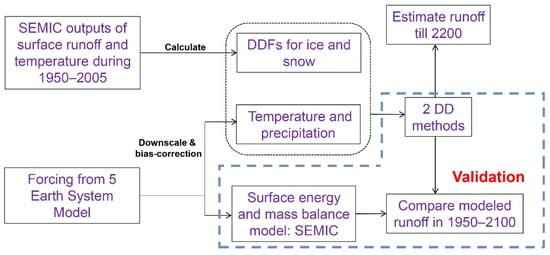
Figure 1.
Flow chart of the study design.
2. Methods
We used both SEMIC and DD models to estimate GrIS surface runoff in the historical period 1950–2005 and the period 2006–2100 under the RCP4.5 and RCP8.5 scenarios. We took SEMIC results as the reference and tuned DD models results (Section 2.3) to match SEMIC results for 1950–2005. We validated the tuned DD models in the period 2006–2100. Finally, we used the tuned DD models to project GrIS runoff from 2101 to 2200 under extension scenarios for RCP4.5 and RCP8.5. The evolution of equilibrium line altitude (ELA), the ice sheet area, and runoff-elevation feedback were considered in the simulations.
2.1. Climate Forcing to 2200
We used five Coupled Model Intercomparison Project Phase 5 (CMIP5) ESM (Table 1) outputs as climate forcing for the period 1950–2005 under the historical scenario, for the period 2006–2100 under RCP4.5 and RCP8.5 scenarios, and for the period 2101–2200 under RCP4.5 and RCP8.5 extension scenarios [32,33,34,35]. RCP4.5 is a mid-range scenario corresponding to a linear increase in radiative forcing towards 4.5 Wm−2 by 2080 and stabilizing by 2100 [36]; this scenario is very policy relevant as it approximates to the Nationally Determined Contributions commitments (NDCs) made by signatories of the Paris climate agreement [37]. RCP8.5 is a high-range scenario with a high radiative forcing level of 8.5 Wm−2 for 2100 [35].

Table 1.
Earth System Models in CMIP5 used in this study.
2.1.1. Prior to 2100
For simulations in the period 1950–2100, the five ESMs (Table 1) outputted the daily mean values of short-wave (SW) and long-wave (LW) radiation downward, near-surface air temperature, surface wind speed, near-surface specific humidity, and snowfall and rainfall available under historical, RCP4.5, and RCP8.5 scenarios.
All five ESMs’ surface temperatures were statistically downscaled to 0.5° × 0.5° grids using a temperature lapse rate of 0.71 °C (100 m)−1, which was derived from automatic weather station (AWS) measurements [42]. Incoming SW and LW radiation, surface wind speed, near-surface specific humidity, surface pressure, and snowfall and rainfall were bi-linearly interpolated into the same 0.5° × 0.5° grid. Secondly, we bias-corrected the downscaled daily data with Inter-Sectoral Impact Model Intercomparison Projection (ISI-MIP; [43]) methods and used the 0.5° × 0.5° ERA-Interim [20] for 1979–2005 as the observation-based reference climate. ERA-Interim has been satisfactorily used in GrIS simulations and has shown a good agreement with observations [20,44]. Finally, we bi-linearly interpolate all climate fields to 0.1° × 0.1° to better follow the ice margin.
We compared downscaled and bias-corrected near-surface air temperature output from the ESMs with the observations from 5 automatic weather station (AWS) sites (Figure S2 and Table S1) from the Greenland Climate Network [42] during 1996–2005. The modeled temperatures agreed well with observations during the spring and autumn but had larger differences in the winter (Figure S3). The runoff from ice melt mainly occurs in the summer and Figure S4 shows that JJA temperatures from ESMs exhibited a similar distribution as the observations, although the highest temperatures were lower than those from the AWSs.
Modeled annual near-surface air temperatures during 1950–2100 for the GrIS are shown in Figure 2a. The modeled temperatures showed no significant trend before 1990 but increased thereafter. The bias-corrected ensemble mean temperature by the year 2100 under RCP4.5 was 4.4 °C higher than during the period 1950–2005, and 9.9 °C higher under RCP8.5 (Figure 2a). Temperatures from the ERA-Interim dataset were temporally and spatially well correlated with bias-corrected modeled temperatures from the ESMs (Figure 2b).
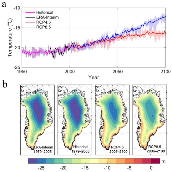
Figure 2.
(a) Five-model ensemble mean annual near-surface air temperatures during 1950–2100 calculated from bias-corrected and downscaled ESM outputs under RCP4.5 (red) and RCP8.5 (blue) scenarios, and ERA-Interim data (black) for the period 1950–2005 (magenta). Colored shading indicates the across-model spread. (b) Maps of near-surface air temperature from ERA-Interim and downscaled ESMs for the period 1979–2005 under the RCP4.5 and RCP8.5 (2006–2100) scenarios.
2.1.2. Post-2100
For the simulations from 2100 to 2200, we used the post-2100 extension scenarios of RCP4.5 ([32,33,34] with constant concentrations after 2150 and a smooth transition between 2100 and 2150 (Figure 3a) and RCP8.5 ([35] with constant emissions after 2100 and constant concentrations after 2250 with a smooth transition of emissions between 2150 and 2250 (Figure 3a). DD models are driven by near-surface air temperature. We found a significant linear relationship between global annual mean radiative forcing (F) and near-surface annual mean air temperature averaged over the GrIS, TF under both RCP4.5 (R = 0.98; p < 0.01) and RCP8.5 (R = 0.99; p < 0.01) during 1950–2100 (Figure 3b,c; Equation (1)).
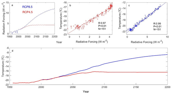
Figure 3.
(a) Annual global radiative forcing under RCP4.5 (red) and RCP8.5 (blue) scenarios. (b,c) GrIS near-surface air temperature as a function of global radiative forcing under RCP4.5 (b) and RCP8.5 (c) from 1950 to 2100. (d) Decadal GrIS temperature change calculated by 5 downscaled ESMs (1950–2100; Table 1) and global radiative forcing (2101–2200) under historical (red, 1950–2005), RCP4.5 (red, 2006–2200), and RCP8.5 (blue, 2006–2200) scenarios.
We assumed that Equation (1) holds from 2101 to 2200. After the year 2100, TF is constant under the RCP4.5 scenario, but increases under the RCP8.5 scenario until the year 2200 with a warming of 4.0 °C relative to 2100 (Figure 3d).
To obtain a daily near-surface air temperature time series at each grid point over the GrIS, Tgrid (t) after 2100, we took 2080–2100 as the baseline for post-2100. We assumed that the post-2100 temperature anomaly relative to the mean temperature for 2080–2100 at each grid point is proportional to the average temperature anomaly over the whole GrIS, and the weight of temperature anomaly at each point is the same as for the 20th century, which is calculated by comparing mean temperatures between 2000–2020 and 2080–2100 for simplicity. Tgrid (t) is calculated by Equation (2) as follows:
or its equivalent form
where j represents the day in a year, t represents the year from 2101 to 2200, and are the 21-year average (2080–2100 and 2000–2020) of daily temperature for the same day at each grid point, , , and TF(t) are annual mean air temperature for the periods 2080–2100, 2000–2020, and the year t = 2101, …, 2200 averaged over all grids points.
2.2. Surface Energy and Mass Balance Model SEMIC
The surface energy and mass balance model SEMIC [16] is efficient in calculating the main surface processes involved in SMB and runoff and has been successfully used to project the GrIS [16,19,45] and small ice cap [46] SMB in the 21th century. The energy balance equation is described as:
where Ceff denotes the effective heat capacity of the snow; α is the surface albedo, that is the average of snow albedo and the background albedo. We considered four methods for calculating snow albedo and two for the background albedos, making 8 parameterizations in all [19]. Surface albedo is mainly affected by the snow thickness, ranging from >5 m with a fresh snow albedo of 0.79 to <2.8 cm when applying the bare ice albedo of 0.41. The impacts of changing dust and black carbon sources are not considered here. The SW↓ and LW↓ are incoming short- and long-wave radiation at the surface. The upwelling long-wave radiation LW↑ is described by the Stefan–Boltzmann law. The HL and HS are surface latent and sensible hear flux, respectively, which are estimated by the respective bulk approach. The residual heat flux QM/R is calculated from ice melting and freezing. The runoff (RF) in SEMIC is considered as surface melting (Melt) plus liquid precipitation (Rainfall) minus refrozen water from rainfall (Rrain), as shown in Equation (5).
We used the same values for all free parameters in SEMIC as in Krapp et al. [16], which performed parameter optimization over the GrIS in comparison to the more sophisticated region climate model, MAR (Modèle Atmosphérique Régional, version 2).
2.3. Degree-Day (DD) Models
Two DD methods were used to calculate GrIS runoff over 1950–2200. The modeled GrIS runoff originates from ablation, which is equal to degree-day factor (DDF) multiplied by accumulated positive daily temperatures or degree-day, dd:
where DDFice,snow is the DDF for ice if surface elevation is below the equilibrium line altitude (ELA), and for snow if above. The DDF calculation is based on SEMIC and considers rain and refreezing processes. The rainfall impacts on runoff are incorporated in the DDF, and we assumed the same processes in the projections of the future.
We calculated dd with 2 methods.
2.3.1. Method 1
Accumulated positive degree-day is provided by:
where T is positive near-surface daily air temperature, T0 is a temperature threshold. The classical method takes T0 = 0 °C. Van den Broeke et al. [24] found that setting T0 to the melting point significantly underestimates the ice melt due to the diurnal cycle, i.e., if one day’s mean temperature is marginally less than 0 °C, melt would still occur in the warm part of the day. They found a smaller T0 (−5 °C) could account for this. Therefore, we took T0 = −5 °C in Method 1.
2.3.2. Method 2
Huybrechts and de Wolde [28] improved the DD method by parameterizing surface temperature (T) as a function of latitude, surface elevation, and time of year, so that:
where σ is a quantity designed to account for the spread of temperatures about the mean caused by random weather fluctuations and the daily diurnal cycle. We took σ as 4.2 °C, the value successfully tested against observations by Rignot et al. [47] and Reeh et al. [48].
2.3.3. Tuning Degree-Day Factors
One shortcoming of the DD method is that it does not explicitly account for insolation changes over the ice surface, which represents an important component of ice melt. Hence, the DDF value is crucial to the accuracy of the modeled runoff. The common values [49] used, DDF of 2.7 mm °C−1 day−1 for snow and 7.2 mm °C−1 day−1 for ice, lead to underestimated runoff, while the SEMIC outputs are quite consistent with the best available estimates during a historical period [19].
Assuming that the SEMIC results in 1950–2005 are accurate, we used the modeled runoff by SEMIC and calculated DD from Method 1 and Method 2 to tune our DDF over the main runoff region (>50 mm yr−1, modeled by SEMIC) based on Equation (6). The results indicated that DDFs show considerable spatial variation both in Method 1 and Method 2 (Figure 4), indicating that a single value cannot be representative for the spatial pattern of DDFs. However, using the deduced historical spatial pattern of DDF in Figure 4 is not possible for the future due to margin retreat and surface lowering, which would both change the DDFs at every location and re-distribute them on the ice sheet according to local factors. To handle the spread of expected DDFs to use in the DD models, we therefore calculated the mean DDF and its standard deviation (Table 2) and separated the DDFsnow and DDFice by the observed mean ELA of 1157 m. The observed ELA does not deviate regionally by >100 m [50,51]. Our estimates for year-by-year ELA from SEMIC over the historical period 1950–2010 had a spatial standard deviation < 270 m (Figure S5).
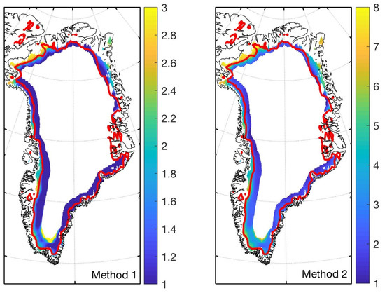
Figure 4.
Tuned DDFs (mm °C−1 day−1) in Method 1 and Method 2. Red lines represent the observed mean ELA of 1127 m.
Table 2.
Tuned mean DDF values (unit: mm °C−1 day−1) for snow and ice and their standard deviation in two DD methods. We used the means of snow and ice plus and minus one standard deviation in the DDF simulations up to 2200 to generate an uncertainty envelope.
2.4. Equilibrium Line Altitude (ELA) Parameterization
The ELA separated the regions using DDFs for ice and snow in our simulation and it evolved every year in our study. We parameterized it for 1950–2200 based on the time series of ELA modeled by SEMIC. There was a significant linear relationship (R = 0.83; Figure 5c) between annual mean modeled ELA (Figure 5a) and ensemble mean near-surface air temperature (Figure 5b) from the bias-corrected and downscaled ESMs (Section 2.1) for the period 1950–2100. We assumed that the same correlation holds for the post-2100 period as that during the period 1950–2100:
where j represents the simulation year from 1950 to 2200.
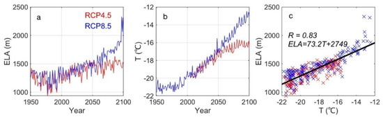
Figure 5.
(a) Modeled annual mean ELAs averaged the whole GrIS by SEMIC during 1950–2100; (b) bias-corrected and downscaled ensemble mean near-surface air temperature over the GrIS during 1950–2100; (c) ELA versus near-surface air temperature (crosses) and linear fit (black line) under RCP4.5 (red crosses) and RCP8.5 (blue crosses).
3. Validation of Tuned DD Methods and Runoff Projections by 2100
Applying the tuned DD methods and ELA parameterization (Section 2.4), we used lower bound, upper bound, and mean values of the DDFs (Table 2) in each of the two DD methods to calculate surface runoff over the whole GrIS during 1950–2100. We did not consider GrIS topography effects and runoff-elevation feedback here for either DD methods or the SEMIC model.
Figure 6 shows the modeled evolution of GrIS runoff under historical, RCP4.5, and RCP8.5 scenarios during 1950–2100. Trends in runoff are consistent with near-surface air temperature over the GrIS (Figure 2a). Before the year 1990, modeled GrIS runoff was at a nearly constant rate. The period prior to the year 1990 has been considered as stable and GrIS mass balance was close to zero [52]. The modeled runoff increased at a rate of 3.5 Gt yr−1 during 1990–2030 under both RCP4.5 and RCP8.5 scenarios. After the year 2030, the modeled runoff under RCP4.5 was lower than that under RCP8.5, consistent with temperature change (Figure 2a).
Modeled runoff over the whole GrIS with DD methods showed good agreement with SEMIC results, especially before 2030, which validates the tuned DD methods (Figure 6). Tuned DD methods provided runoffs of about 20 Gt yr−1 and 98 Gt yr−1 less than SEMIC during 2050–2100 under RCP4.5 and RCP8.5, respectively. The relative difference in runoff between tuned DD and SEMIC during 2050–2089 were 3% (RCP4.5) and 12% (RCP8.5); this compares with the 30% difference between untuned DD methods and SEMIC [19].
The spatial distributions of runoff modeled by SEMIC and DD were very similar (Figure 7 and Figure 8) with very high runoff gradients along the margins where the surface elevation gradient is large and warm ocean influence is greatest.
Our DD runoff is close to the MAR results driven by ERA-Interim [18] during 1980–1990 (Figure 6). However, both are smaller (Figure 6) than the runoff estimated by the SICOPOLIS ice dynamics model bi-directionally coupled to the ECHAM5/MPI-OM atmosphere–ocean climate model [53]. We found similar offsets for the RCP scenarios during 2080–2099 (Table 3).
Table 3.
Mean and standard deviation of modeled runoff by DD methods and SEMIC, and comparisons with different studies under historical and RCP scenarios (Gt yr−1).

Figure 6.
Decadal GrIS runoff estimated by the average of two DD models (solid lines) and SEMIC (dashed lines) during 1950–2100 under historical (magenta), RCP4.5 (red), and RCP8.5 (blue) scenarios. Both SEMIC (mean of 8 albedo parameterizations) and DD results are driven by five ESMs. Colored shadings indicate the results spread in different DDF values. The grey boxed region is from MAR model results (Fettweis et al. [18]); the yellow boxed regions are from Vizcaino et al. [54].

Figure 7.
Spatial distribution of annual mean GrIS runoff during 1950–2005 (1st column), 2006–2030 (2nd column), and 2080–2100 (3rd column) estimated by SEMIC as the mean of eight albedo parameterizations under RCP4.5 (top row) and RCP8.5 (bottom row), and anomalies relative to 1950–2005 for 2006–2030 (4th column) and 2080–2100 (last column).

Figure 8.
As for Figure 7, but the mean is estimated by two DD methods.
4. Results
4.1. Runoff-Elevation Feedback and Ice Area Evolution
We did not consider runoff-elevation feedback or ice area evolution in the simulations to 2100 using both DD methods and SEMIC. However, both may have a significant effect on modeled runoff over a longer future simulation to 2200. Our initial topographic data derived from Morlighem et al. [54] for the period 1993–2016 with the same spatial resolution as SEMIC input and we assumed it could also represent the GrIS over the 1950–2005 when we assumed that the GrIS was in an equilibrium state.
We estimated the upper bound for the runoff-elevation feedback over the period 2006–2200 based on the assumption of constant ice dynamics. To estimate the rate of ice dynamic submergence/emergence velocity, we assumed a steady state for the historical period 1950–2005; that is, we assumed that the surface elevation change was zero over that time-period and the surface mass balance was exactly balanced by the submergence/emergence velocity of the ice. We therefore used the mean SMB over that time-period as a proxy for the ice dynamic submergence/emergence velocity, and we computed surface height changes moving forward in time under the assumption that only deviations in SMB from the historical mean would produce surface height changes. This assumption is unlikely to be exactly correct, but it still represents an improvement over neglecting ice dynamics entirely. For our purposes, it is sufficient to state that this method was likely going to overestimate surface height changes due to SMB as the ice sheet flow would adjust to counteract the changing SMB over a timescale of centuries [55]. Clearly, this method neglects the potential for ice dynamic changes due to outlet glacier retreat or other unsteady ice dynamic processes. However, that was not our purpose in using this method. Instead, we were attempting to set an upper bound on the amount of surface height change that might be expected from the runoff-elevation feedback, and this method is well suited to that task.
To do this, we let represent the historical average net SMB (Equation (10)). We then computed the height change at future times based on the temporal integrity of the anomaly of SMB relative to the historical value (Equations (11) and (12)). We then adjusted the surface temperature to account for the computed height change using a constant lapse rate (Equation (13)). Finally, we adjusted the ice mask to remove marginal regions in which the adjusted ice thickness was less than zero (Equation (14)).
We assumed that runoff (RF, unit: m w.e. s−1), snowfall (SF, unit: m w.e. s−1), and historical surface elevation change caused by ice dynamics (historical modeled runoff (RFhis) minus snowfall (SFhis)) are the dominant factors that affect GrIS topography in the period 2006–2200, which includes changes in surface elevation (H), ice thickness (Hice thickness), and ice sheet boundary changes (Mask). We further assumed that for each day since the start of 2006, changes in the surface elevation () over the whole GrIS were due to the difference between SF and RF (Equation (11)), leading to an updated H (Equation (12)) and an updated near-surface air temperature (Tfeedback). This would be based on downscaled and bias-corrected near-surface air temperature output from ESMs (TESM) on the initial surface topography and a lapse rate () of 7.1 °C km−1 (Equation (13)), as observed in [42]. Mask is determined by ice thickness in Equation (14).
where j represents j days since the start of 2006, H0 represents initial surface elevation, and represents initial ice thickness.
During the period 2006–2100, snowfall (SF) originated from the five sets of downscaled and bias-corrected ESM outputs. Three ESMs (BNU-ESM, MIROC-ESM, and MIROC-ESM-CHEM) showed no significant trend in snowfall (Figure S1), while CanESM2 and HadGEM-2-ES showed significant (Mann–Kendall test at 95% level during 1950–2100) rises in snowfall under RCP4.5. Only HadGEM2-ES showed a significant rise in snowfall under RCP8.5. Annual average snowfall projected by CanESM2 during 2091–2100 was 9% more than that for 2011–2020, while that by HadGEM2-ES was 11% more under RCP4.5 and 20% more under RCP8.5.
We kept the same daily SF for the period 2101–2200 as the annual mean daily snowfall for the period 2080–2100 under each scenario. We also tested runoff sensitivity to snowfall amount in the post-2100 period by also simulating 150% snowfall of the 2080–2100 period and with 200% of its snowfall.
4.2. Runoff Projections to 2200
Figure 9 shows the modeled runoff over the GrIS with tuned DD methods under RCP4.5 and RCP8.5, with both runoff-elevation feedback and ice area change included. Runoff-elevation feedback acts to increase modeled runoff, while reduced ice area decreases modeled runoff. Modeled runoff including these two effects was larger than what we calculated in Section 3 to the year 2100 by 4% under RCP4.5 and by 2% under RCP8.5. This indicates that runoff-elevation feedback dominates the reduction in ice area. Ice area was reduced by 2% under RCP4.5 and RCP8.5 by 2100.
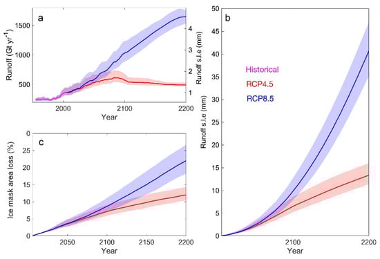
Figure 9.
(a) Modeled annual runoff by the average of two DD methods in the period 1950–2005 under the historical scenario (magenta), and 2006–2200 under RCP4.5 (red) and RCP8.5 (blue) and their extensions. (b) Cumulative runoff equivalent to global mean sea-level rise during 2006–2200 under RCP4.5 (red) and RCP8.5 (blue) relative to 1950–2005. (c) Same as (b), however for ice area loss. Colored shading indicates the spread using different DDFs.
Under RCP4.5, the modeled runoff peaked at 605 Gt yr−1 in the year 2088 and then gradually decreased by 493 Gt yr−1 by 2200 (Figure 9a). Under RCP8.5, the runoff increased by 1650 Gt yr−1 in the year 2200, over twice that under RCP4.5. This is reflected in the cumulative contributions to global mean sea-level rise from GrIS runoff (Figure 9b). By 2100, modeled sea-levels rise by 6 ± 2 cm (RCP4.5) and 9 ± 3 cm (RCP8.5) relative to the 1950–2005 period and by 13 ± 4 cm (RCP4.5) and 40 ± 5 cm (RCP8.5) by 2200. The spatial distribution of runoff is shown in Figure 10; as with 2100, the runoff region is mainly from around the margins of the GrIS.
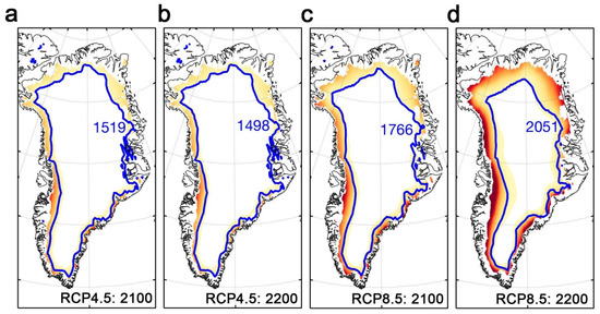
Figure 10.
Multi-model mean runoff estimated by two DD methods in 2100 (a,c) and 2200 (b,d) under RCP4.5, RCP8.5, and their extensions. Blue curves represent equilibrium line, and numbers in blue are ELA (m).
ELA increased and peaked in the year 2100 under RCP4.5 and in the year 2200 under RCP8.5, similar to the corresponding temperature time series. The ELA trend was monotonically downwards under RCP4.5 after 2100, while the ELA trend rose under RCP8.5 (Figure 10). This is because RCP4.5 peak radiative forcing and temperatures occur before 2100 (Figure 3a,d), driving ELA upwards until then. However, the constant radiative forcing after 2100 (Figure 3a) together with increased snowfall, notably in HadGEM2-ES (Figure S1), act to decrease surface temperatures because elevation rises quicker than the runoff lowers elevations. Under RCP8.5, ELA rose with radiative forcing and temperatures by 2200 (Figure 3).
Tests with increased snowfall lead to increased runoff. A 150% increase (relative to 2080–2100) yielded a 10% increase in runoff, and a 200% increase in snowfall produced 20% additional runoff under RCP4.5 by the year 2200. Under RCP8.5, the increases were 5% and 10%. The greater ice area lost under RCP8.5 compared with RCP4.5 (Figure 9c), dominates over the increased snowfall expected as it also does the elevation feedback. To study the impact of runoff-elevation feedback alone, we also made simulations to 2200 only accounting for ice area change and without runoff-elevation feedback. Comparing results with and without runoff-elevation feedback, we found that runoff-elevation feedback contributes 5 ± 2% (RCP4.5) and 6 ± 2% (RCP8.5) additional runoff by 2100, and 12 ± 4% (RCP4.5) and 15 ± 5% (RCP8.5) by 2200 (Figure 11).
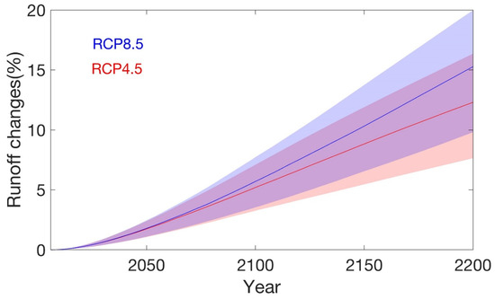
Figure 11.
Percentage of runoff changes caused by runoff-elevation feedback by the average of two DD methods under RCP4.5 (red) and RCP8.5 (blue) scenarios. Colored shading indicates the spread from different DDFs.
5. Discussion
We simulated surface runoff changes for the GrIS to the year 2200 and estimated the runoff-elevation feedback under the assumption of constant ice dynamics. While mass loss driven by the retreat of ocean-terminating outlet glaciers has been important in the recent past and may be an important factor in the coming century, models indicate that, over the longer-term, dynamic retreat is likely to be a self-limiting process as important glaciers retreat out of contact with the ocean, leaving surface mass balance as the dominant control on GrIS evolution after the year 2100 [6,25]. Thus, our estimated runoff changes and our estimate of the upper limit of the runoff-elevation feedback are likely to be robust, especially in the longer term.
Our estimated runoff contributions under RCP8.5 by the year 2100, 9 ± 3 cm were very close to the results of the Ice Sheet Model Intercomparison Project (89 ± 51 mm), which used a large ensemble of models with atmospheric and oceanic forcing and ice dynamics [56], and ~2 cm lower than dynamic projections by Fürst et al. [6]. By the year 2200, our runoff was 56% lower than Vizcaino et al. [54], which applied coupled simulations considering the changes in ice dynamics and elevation-surface mass balance feedback.
For simplicity, we did not consider the impact of topography on the spatial pattern and the type of precipitation that may change the ratio of rainfall and snowfall [57]. In addition, applying a uniform ELA over the whole GrIS ignored that the western GrIS is expected to melt earlier and faster than other regions in a warmer climate, hence our study may have underestimated the western GrIS runoff.
We statistically extrapolated the temperature (beyond 2100) from the annual radiative forcing for extensive RCP scenarios. This is not accurate enough as it lacks substantial physically atmospheric processes. Although extensions beyond 2100 are available for several CMIP5 ESMs, and the recent, newly released climate datasets are available up to 2500 [58], they cannot simulate a realistic climate for Greenland as the elevation of the ice sheet will likely deviate significantly from the topography condition configured by the ESMs [59].
Sea-level rise is estimated to be 1.84–5.48 m by the year 2200 under different climate scenarios [60]. GrIS mass loss remains a large source of uncertainty for sea-level rise in the future [5]. Both uncertainty and projected sea-level rise will rapidly increase beyond 2100 [61] as surface runoff will increase the non-linearly with temperatures under scenarios with high CO2 emissions [62]. The large, scenario-dependent differences in mass loss from the GrIS will remain on millennial timescales because warm scenarios could lead to irreversibly larger mass loss due to the positive SMB-elevation feedback if summer temperatures rise ~1.5–2 °C above pre-industrial levels [63] for a sustained period. Existing studies show that the GrIS will likely disappear within a millennium without substantial net reductions in greenhouse gas emissions [25].
The positive runoff-elevation feedback over the GrIS has been estimated in many studies [19,53,64]. In this study, runoff-elevation feedback would produce 5 ± 2% (RCP4.5) and 6 ± 2% (RCP8.5) additional runoff by 2100. Vizcaino et al. [54] estimated increases of 10% (RCP4.5) and 8% (RCP8.5) in loses due to SMB-elevation feedback by 2100, which are almost double our results.
Near-surface air temperature is the main factor affecting ice sheet changes, but snowfall indirectly has an impact on GrIS runoff by changing surface elevation and then changing near-surface air temperature. Some studies have pointed out that the snowfall over Greenland will increase under 21st century warming conditions [18]. Among all five ESMs used in this study, only HadGEM2-ES projected an increasing trend in snowfall under both RCP4.5 and RCP8.5. Despite this, we explored runoff sensitivity to the choice of snowfall. The results showed that increased snowfall will lead to increased runoff; the double snowfall increase under RCP4.5 and RCP8.5 will lead to an increase of 22% and 13% in runoff, respectively.
We assumed that climate insolation will not change from the present day to 2200. The DD method is inadequate for long-term modelling, e.g., Quaternary glacial cycles, as it does not explicitly consider the short-wave radiation absorbed by the surface. This can lead to a significant underestimation of the effect of varying insolation on orbital timescales, which is the key driver of the glacial cycles [65,66]. Van de Berg et al. [67] showed that short-wave changes caused Eemian melt rates to be twice those attributable to air temperature rises alone. While orbital dynamics will not significantly affect solar radiation on the timescales we have studied, air-borne pollution may over the coming centuries. The emissions of pollutants, especially black carbon from industry, as well as natural sources may rise because of anthropogenic emissions related to increased energy consumption and rising temperatures leading to increased fire outbreaks, especially in the boreal forest zone. Black carbon produces a significant darkening of snow surfaces, even at concentrations of parts per billion, and the influence of black carbon on temperature and the melting of snow is three times greater than that of CO2 in Arctic regions [68]. Hence, changes in aerosol emissions are likely to produce changes in the DDFs over the coming centuries, especially for snow. It is also possible that pro-active emission and pollution control, especially in Asia, will lead to declines in aerosol load this century. In our simulations, the DDFs for snow played a less critical role than ablation in the marginal areas of the ice sheet. The region above ELA produced about 20–30% total runoff after the year 2100, meaning that DDFs for ice and their uncertainties dominate future, warmer climate runoff estimates. The ESMs we used simulated 8% (RCP4.5) and 25% (RCP8.5) increases in rain and corresponding decreases in snowfall for 2100 compared with 2000 over the GrIS. Rain on snow is an active topic of research because it affects both ecology and albedo. The effects of rain on snow would be most important at higher elevations where it converts snow more rapidly into ice than would otherwise occur. Simulating such process requires a more sophisticated snowpack energy balance model, such as SNICAR [68], and which are not fully incorporated in any ESM at present.
6. Conclusions
We simulated and projected runoff over the GrIS from 1950 to 2200 using two tuned Degree-Day methods, forced with bias-corrected and downscaled near-surface temperatures and snowfall from five Earth System Models under the scenarios of RCP4.5, RCP8.5, and their extensions. The DDF values in DD methods were tuned using SEMIC model results and validated over the whole GrIS for the period 1950–2100; they were then applied in the projection to the year 2200. ELA was parameterized as a function of mean near-surface air temperature, and runoff-elevation feedback and ice area evolution were considered in our post-2005 simulations. Runoff-elevation feedback, which acts to increase modeled runoff, dominates the reduction in ice area, which decreases the modeled runoff. The accumulated runoff in global mean sea-level equivalent rises by 6 ± 2 cm under RCP4.5 and 9 ± 3 cm under RCP8.5 by the year 2100, and 13 ± 4 cm under RCP4.5 and 40 ± 5 cm under RCP8.5 by 2200 relative to the period 1950–2005. Runoff-elevation feedback increases the extra runoff by 5 ± 2% (RCP4.5) and 6 ± 2% (RCP8.5) by 2100 and by 12 ± 4% (RCP4.5) and 15 ± 5% (RCP8.5) by 2200.
Supplementary Materials
The following are available online at https://www.mdpi.com/article/10.3390/atmos12121569/s1, Figure S1: Downscaled and bias-corrected snowfall from BNU-ESM (red), CanESM2 (blue), HadGEM2-ES (magenta), MIROC-ESM (cyan) and MIROC-ESM-CHEM (black) under RCP4.5 (a) and RCP8.5 (b) during 1950–2100. Thick curves indicate that significant trend in snowfall through Mann-Kendall test at 95% level, Figure S2: Map of AWS observations over GrIS, Figure S3: Historical monthly near-surface air temperature over GrIS site Swiss Camp (a), Humboldt (b), Summit (c), TUNU-N (d) and South Dome (e) from BNU-ESM (red), CanESM2 (magenta), HadGEM2-ES (blue), MIROC-ESM (cyan), MIROC-ESM-CHEM (black) and AWS observation (gray). ESMs are downscaled and bias-corrected by ISI-MIP. Note that Swiss Camp and Humboldt are during the period of 1996–2005, Summit and TUNU-N are 1997–2005, South Dome is 1998–2005, Figure S4: Scatter plot of historical summer season (JJA) monthly mean near-surface air temperature (°C) that downscaled and bias-corrected from BNU-ESM (red), CanESM2 (magenta), HadGEM2-ES (blue), MIROC-ESM (cyan) and MIROC-ESM-CHEM (black) versus that observed by AWS over GrIS site Swiss Camp, Humboldt, Summit, TUNU-N and South Dome. Solid green line shows the one-to-one line and dotted line shows linear fitted line by 5 ESMs. Note that temperatures at Swiss Camp and Humboldt were observed during the period 1996–2005, Summit and TUNU-N 1997–2005, South Dome 1998–2005, Figure S5: Annual standard deviation of ELA over GrIS modeled by SEMIC from ensemble mean of BNU-ESM, HadGEM2-ES, MIROC-ESM, MIROC-ESM-CHEM and CanESM2, Table S1: AWS position over GrIS.
Author Contributions
Conceptualization, C.Y. and L.Z.; methodology, C.Y., M.W., J.C.M. and L.Z.; software, C.Y.; validation, C.Y.; formal analysis, C.Y.; investigation, C.Y.; resources, C.Y.; data curation, C.Y.; writing—original draft preparation, C.Y.; writing—review and editing, C.Y., L.Z., J.C.M. and M.W.; visualization, C.Y.; supervision, L.Z. and J.C.M.; project administration, L.Z. and J.C.M.; funding acquisition, L.Z. and J.C.M. All authors have read and agreed to the published version of the manuscript.
Funding
This work was funded by the National Key Research and Development Program of China (2018YFC1406104) and the National Natural Science Foundation of China (No. 41941006).
Institutional Review Board Statement
Not applicable.
Informed Consent Statement
Not applicable.
Data Availability Statement
Not applicable.
Conflicts of Interest
The authors declare no conflict of interest.
References
- Lenton, T.M.; Held, H.; Kriegler, E.; Hall, J.W.; Lucht, W.; Rahmstorf, S.; Schellnhuber, H.J. Tipping elements in the Earth’s climate system. Proc. Natl. Acad. Sci. USA 2008, 105, 1786–1793. [Google Scholar] [CrossRef]
- Van den Broeke, M.R.; Enderlin, E.M.; Howat, I.M.; Kuipers Munneke, P.; Noël, B.P.Y.; Jan Van De Berg, W.; Van Meijgaard, E.; Wouters, B. On the recent contribution of the Greenland ice sheet to sea level change. Cryosphere 2016, 10, 1933–1946. [Google Scholar] [CrossRef]
- Csatho, B.M.; Schenk, A.F.; van der Veen, C.J.; Babonis, G.; Duncan, K.; Rezvanbehbahani, S.; Van Den Broeke, M.R.; Simonsen, S.B.; Nagarajan, S.; van Angelen, J.H. Laser altimetry reveals complex pattern of Greenland Ice Sheet dynamics. Proc. Natl. Acad. Sci. USA 2014, 111, 18478–18483. [Google Scholar] [CrossRef]
- Enderlin, E.M.; Howat, I.M.; Jeong, S.; Noh, M.; van Angelen, J.H.; van den Broeke, M.R. An improved mass budget for the Greenland ice sheet. Geophys. Res. Lett. 2014, 41, 866–872. [Google Scholar] [CrossRef]
- Church, J.A.; White, N.J. Sea-level rise from the late 19th to the early 21st century. Surv. Geophys. 2011, 32, 585–602. [Google Scholar] [CrossRef]
- Fürst, J.J.; Goelzer, H.; Huybrechts, P. Ice-dynamic projections of the Greenland ice sheet in response to atmospheric and oceanic warming. Cryosphere 2015, 9, 1039–1062. [Google Scholar] [CrossRef]
- Wilton, D.J.; Jowett, A.; Hanna, E.; Bigg, G.R.; Van Den Broeke, M.R.; Fettweis, X.; Huybrechts, P. High resolution (1 km) positive degree-day modelling of Greenland ice sheet surface mass balance, 1870–2012 using reanalysis data. J. Glaciol. 2017, 63, 176–193. [Google Scholar] [CrossRef][Green Version]
- Kraaijenbrink, P.D.A.; Bierkens, M.F.P.; Lutz, A.F.; Immerzeel, W.W. Impact of a global temperature rise of 1.5 degrees Celsius on Asia’s glaciers. Nature 2017, 549, 257–260. [Google Scholar] [CrossRef]
- Zhao, L.; Tian, L.; Zwinger, T.; Ding, R.; Zong, J.; Ye, Q.; Moore, J.C. Numerical simulations of Gurenhekou glacier on the Tibetan Plateau. J. Glaciol. 2014, 60, 71–82. [Google Scholar] [CrossRef]
- Zhang, Y.; Liu, S.; Ding, Y. Observed degree-day factors and their spatial variation on glaciers in western China. Ann. Glaciol. 2006, 43, 301–306. [Google Scholar] [CrossRef]
- Hanna, E.; Huybrechts, P.; Cappelen, J.; Steffen, K.; Bales, R.C.; Burgess, E.; McConnell, J.R.; Steffensen, J.P.; Van Den Broeke, M.; Wake, L.; et al. Greenland Ice Sheet surface mass balance 1870 to 2010 based on Twentieth Century Reanalysis, and links with global climate forcing. J. Geophys. Res. Atmos. 2011, 116, 1–20. [Google Scholar] [CrossRef]
- Box, J.E.; Cressie, N.; Bromwich, D.H.; Jung, J.H.; Van Den Broeke, M.; Van Angelen, J.H.; Forster, R.R.; Miège, C.; Mosley-Thompson, E.; Vinther, B.; et al. Greenland ice sheet mass balance reconstruction. Part I: Net snow accumulation (1600–2009). J. Clim. 2013, 26, 3919–3934. [Google Scholar] [CrossRef]
- Braithwaite, R.J. Positive degree-day factors for ablation on the Greenland ice sheet studied by energy-balance modelling. J. Glaciol. 1995, 41, 153–160. [Google Scholar] [CrossRef]
- Vincent, C.; Six, D. Relative contribution of solar radiation and temperature in enhanced temperature-index melt models from a case study at Glacier de Saint-Sorlin, France. Ann. Glaciol. 2013, 54, 11–17. [Google Scholar] [CrossRef]
- Gabbi, J.; Carenzo, M.; Pellicciotti, F.; Bauder, A.; Funk, M. A comparison of empirical and physically based glacier surface melt models for long-term simulations of glacier response. J. Glaciol. 2014, 60, 1140–1154. [Google Scholar] [CrossRef]
- Krapp, M.; Robinson, A.; Ganopolski, A. SEMIC: An efficient surface energy and mass balance model applied to the Greenland ice sheet. Cryosphere 2017, 11, 1519–1535. [Google Scholar] [CrossRef]
- Noël, B.; Van De Berg, W.J.; Van Meijgaard, E.; Kuipers Munneke, P.; Van De Wal, R.S.W.; Van Den Broeke, M.R. Evaluation of the updated regional climate model RACMO2. 3: Summer snowfall impact on the Greenland Ice Sheet. Cryosphere 2015, 9, 1831–1844. [Google Scholar] [CrossRef]
- Fettweis, X.; Franco, B.; Tedesco, M.; Van Angelen, J.H.; Lenaerts, J.T.M.; van den Broeke, M.R.; Gallée, H. Estimating the Greenland ice sheet surface mass balance contribution to future sea level rise using the regional atmospheric climate model MAR. Cryosphere 2013, 7, 469–489. [Google Scholar] [CrossRef]
- Moore, J.C.; Yue, C.; Zhao, L.; Guo, X.; Watanabe, S.; Ji, D. Greenland ice sheet response to stratospheric aerosol injection geoengineering. Earth’s Future 2019, 7, 1451–1463. [Google Scholar] [CrossRef]
- Simmons, A. ERA-Interim: New ECMWF reanalysis products from 1989 onwards. ECMWF Newsl. 2006, 110, 25–36. [Google Scholar]
- Plach, A.; Nisancioglu, K.H.; Le Clec’h, S.; Born, A.; Langebroek, P.M.; Guo, C.; Imhof, M.; Stocker, T.F. Eemian Greenland SMB strongly sensitive to model choice. Clim. Past 2018, 14, 1463–1485. [Google Scholar] [CrossRef]
- Peano, D.; Colleoni, F.; Quiquet, A.; Masina, S. Ice flux evolution in fast flowing areas of the Greenland ice sheet over the 20th and 21st centuries. J. Glaciol. 2017, 63, 499–513. [Google Scholar] [CrossRef][Green Version]
- Hock, R. Temperature index melt modelling in mountain areas. J. Hydrol. 2003, 282, 104–115. [Google Scholar] [CrossRef]
- Van Den Broeke, M.; Bus, C.; Ettema, J.; Smeets, P. Temperature thresholds for degree-day modelling of Greenland ice sheet melt rates. Geophys. Res. Lett. 2010, 37, L18501. [Google Scholar] [CrossRef]
- Aschwanden, A.; Fahnestock, M.A.; Truffer, M.; Brinkerhoff, D.J.; Hock, R.; Khroulev, C.; Mottram, R.; Abbas Khan, S. Contribution of the Greenland Ice Sheet to sea level over the next millennium. Sci. Adv. 2019, 5, eaav9396. [Google Scholar] [CrossRef]
- Van Breedam, J.; Goelzer, H.; Huybrechts, P. Semi-equilibrated global sea-level change projections for the next 10,000 years. Earth Syst. Dyn. Discuss. 2020, 11, 953–976. [Google Scholar] [CrossRef]
- Clark, P.U.; Shakun, J.D.; Marcott, S.A.; Mix, A.C.; Eby, M.; Kulp, S.; Levermann, A.; Milne, G.A.; Pfister, P.L.; Santer, B.D.; et al. Consequences of twenty-first-century policy for multi-millennial climate and sea-level change. Nat. Clim. Chang. 2016, 6, 360–369. [Google Scholar] [CrossRef]
- Huybrechts, P.; de Wolde, J. The dynamic response of the Greenland and Antarctic ice sheets to multiple-century climatic warming. J. Clim. 1999, 12, 2169–2188. [Google Scholar] [CrossRef]
- Driesschaert, E.; Fichefet, T.; Goosse, H.; Huybrechts, P.; Janssens, I.; Mouchet, A.; Munhoven, G.; Brovkin, V.; Weber, S.L. Modeling the influence of Greenland ice sheet melting on the Atlantic meridional overturning circulation during the next millennia. Geophys. Res. Lett. 2007, 34, L10707. [Google Scholar] [CrossRef]
- Mengel, M.; Nauels, A.; Rogelj, J.; Schleussner, C.-F. Committed sea-level rise under the Paris Agreement and the legacy of delayed mitigation action. Nat. Commun. 2018, 9, 601. [Google Scholar] [CrossRef]
- Lowe, J.A.; Gregory, J.M.; Ridley, J.; Huybrechts, P.; Nicholls, R.J.; Collins, M. The role of sea-level rise and the Greenland ice sheet in dangerous climate change: Implications for the stabilisation of climate. Avoid. Danger. Clim. Chang. 2006, 29, 36. [Google Scholar]
- Golledge, N.R.; Keller, E.D.; Gomez, N.; Naughten, K.A.; Bernales, J.; Trusel, L.D.; Edwards, T.L. Global environmental consequences of twenty-first-century ice-sheet melt. Nature 2019, 566, 65–72. [Google Scholar] [CrossRef] [PubMed]
- Clarke, L.; Edmonds, J.; Jacoby, H.; Pitcher, H.; Reilly, J.; Richels, R. Scenarios of Greenhouse Gas Emissions and Atmospheric Concentrations; Department of Energy, Office of Biological & Environment Research: Washington, DC, USA, 2007; p. 154. [Google Scholar]
- Smith, S.J.; Wigley, T.M.L. Multi-gas forcing stabilization with Minicam. Energy J. 2006, 27, 373–392. [Google Scholar] [CrossRef]
- Wise, M.; Calvin, K.; Thomson, A.; Clarke, L.; Bond-Lamberty, B.; Sands, R.; Smith, S.J.; Janetos, A.; Edmonds, J. Implications of limiting CO2 concentrations for land use and energy. Science 2009, 324, 1183–1186. [Google Scholar] [CrossRef]
- Riahi, K.; Rao, S.; Krey, V.; Cho, C.; Chirkov, V.; Fischer, G.; Kindermann, G.; Nakicenovic, N.; Rafaj, P. RCP 8.5—A scenario of comparatively high greenhouse gas emissions. Clim. Chang. 2011, 109, 33. [Google Scholar] [CrossRef]
- Thomson, A.M.; Calvin, K.V.; Smith, S.J.; Kyle, G.P.; Volke, A.; Patel, P.; Delgado-Arias, S.; Bond-Lamberty, B.; Wise, M.A.; Clarke, L.E. RCP 4.5: A pathway for stabilization of radiative forcing by 2100. Clim. Chang. 2011, 109, 77. [Google Scholar] [CrossRef]
- Kitous, A.; Keramidas, K. Analysis of Scenarios Integrating the INDCs; European Comission: Brussels, Belgium, 2015. [Google Scholar]
- Ji, D.; Wang, L.; Feng, J.; Wu, Q.; Cheng, H.; Zhang, Q.; Yang, J.; Dong, W.; Dai, Y.; Gong, D. Description and basic evaluation of Beijing Normal University Earth system model (BNU-ESM) version 1. Geosci. Model Dev. 2014, 7, 2039–2064. [Google Scholar] [CrossRef]
- Arora, V.K.; Scinocca, J.F.; Boer, G.J.; Christian, J.R.; Denman, K.L.; Flato, G.M.; Kharin, V.V.; Lee, W.G.; Merryfield, W.J. Carbon emission limits required to satisfy future representative concentration pathways of greenhouse gases. Geophys. Res. Lett. 2011, 38, L05805. [Google Scholar] [CrossRef]
- Collins, W.J.; Bellouin, N.; Doutriaux-Boucher, M.; Gedney, N.; Halloran, P.; Hinton, T.; Hughes, J.; Jones, C.D.; Joshi, M.; Liddicoat, S. Development and evaluation of an Earth-System model–HadGEM2. Geosci. Model Dev. 2011, 4, 1051–1075. [Google Scholar] [CrossRef]
- Watanabe, S.; Hajima, T.; Sudo, K.; Nagashima, T.; Takemura, T.; Okajima, H.; Nozawa, T.; Kawase, H.; Abe, M.; Yokohata, T. MIROC-ESM 2010: Model description and basic results of CMIP5-20c3m experiments. Geosci. Model Dev. 2011, 4, 845–872. [Google Scholar] [CrossRef]
- Steffen, K.; Box, J. Surface climatology of the Greenland ice sheet: Greenland Climate Network 1995–1999. J. Geophys. Res. Atmos. 2001, 106, 33951–33964. [Google Scholar] [CrossRef]
- Hempel, S.; Frieler, K.; Warszawski, L.; Schewe, J.; Piontek, F. A trend-preserving bias correction–the ISI-MIP approach. Earth Syst. Dyn. 2013, 4, 219–236. [Google Scholar] [CrossRef]
- Rignot, E.; Velicogna, I.; van den Broeke, M.R.; Monaghan, A.; Lenaerts, J.T.M. Acceleration of the contribution of the Greenland and Antarctic ice sheets to sea level rise. Geophys. Res. Lett. 2011, 38, L05503. [Google Scholar] [CrossRef]
- Rückamp, M.; Falk, U.; Frieler, K.; Lange, S.; Humbert, A. The effect of overshooting 1.5 °C global warming on the mass loss of the Greenland ice sheet. Earth Syst. Dyn. 2018, 9, 1169–1189. [Google Scholar] [CrossRef]
- Yue, C.; Schmidt, L.S.; Zhao, L.; Wolovick, M.; Moore, J.C. Vatnajökull mass loss under solar geoengineering due to the North Atlantic meridional overturning circulation. Earth’s Future 2021, 9, e2021EF002052. [Google Scholar] [CrossRef]
- Rignot, E.J.; Gogineni, S.P.; Krabill, W.B.; Ekholm, S. North and northeast Greenland ice discharge from satellite radar interferometry. Science 1997, 276, 934–937. [Google Scholar] [CrossRef]
- Reeh, N.; Mayer, C.; Miller, H.; Thomsen, H.H.; Weidick, A. Present and past climate control on fjord glaciations in Greenland: Implications for IRD-deposition in the sea. Geophys. Res. Lett. 1999, 26, 1039–1042. [Google Scholar] [CrossRef]
- Janssens, I.; Huybrechts, P. The treatment of meltwater retention in mass-balance parameterization of the Greenland ice sheet. Ann. Glaciol. 2000, 31, 133–140. [Google Scholar] [CrossRef]
- Haeberli, W. Fluctuations of Glaciers, 1975–1980 (Vol. IV); International Commission on Snow and Ice of the International Association of Hydrological Sciences and UNESCO; Associa-tion of Hydrological Sciences: Paris, France, 1985; ISBN 9231023675. [Google Scholar]
- Weidick, A.; Boggild, C.E.; Knudsen, N.T. Glacier inventory and atlas of West Greenland. Rapp. Grønlands Geol. Undersøgelse 1992, 158, 1–194. [Google Scholar] [CrossRef]
- Rignot, E.; Kanagaratnam, P. Changes in the velocity structure of the Greenland Ice Sheet. Science 2006, 311, 986–990. [Google Scholar] [CrossRef] [PubMed]
- Vizcaino, M.; Mikolajewicz, U.; Ziemen, F.; Rodehacke, C.B.; Greve, R.; Van Den Broeke, M.R. Coupled simulations of Greenland Ice Sheet and climate change up to AD 2300. Geophys. Res. Lett. 2015, 42, 3927–3935. [Google Scholar] [CrossRef]
- Morlighem, M.; Williams, C.N.; Rignot, E.; An, L.; Arndt, J.E.; Bamber, J.L.; Catania, G.; Chauché, N.; Dowdeswell, J.A.; Dorschel, B. BedMachine v3: Complete bed topography and ocean bathymetry mapping of Greenland from multibeam echo sounding combined with mass conservation. Geophys. Res. Lett. 2017, 44, 11–51. [Google Scholar] [CrossRef]
- Winkelmann, R.; Levermann, A.; Martin, M.A.; Frieler, K. Increased future ice discharge from Antarctica owing to higher snowfall. Nature 2012, 492, 239–242. [Google Scholar] [CrossRef] [PubMed]
- Gregory, J.; George, S.; Smith, R. Large and irreversible future decline of the Greenland ice-sheet. Cryosphere 2020, 14, 4299–4322. [Google Scholar] [CrossRef]
- Nowicki, S.; Goelzer, H.; Seroussi, H.; Payne, A.J.; Lipscomb, W.H.; Abe-Ouchi, A.; Agosta, C.; Alexander, P.; Asay-Davis, X.S.; Barthel, A. Experimental protocol for sea level projections from ISMIP6 stand-alone ice sheet models. Cryosphere 2020, 14, 2331–2368. [Google Scholar] [CrossRef]
- Lyon, C.; Saupe, E.E.; Smith, C.J.; Hill, D.J.; Beckerman, A.P.; Stringer, L.C.; Marchant, R.; McKay, J.; Burke, A.; O’Higgins, P. Climate change research and action must look beyond 2100. Glob. Chang. Biol. 2021, 1–13. [Google Scholar] [CrossRef]
- Goelzer, H.; Nowicki, S.; Payne, A.; Larour, E.; Seroussi, H.; Lipscomb, W.; Gregory, J.; Abe-Ouchi, A.; Shepherd, A.; Simon, E.; et al. The future sea-level contribution of the Greenland ice sheet: A multi-model ensemble study of ISMIP6. Cryosphere 2020, 14, 3071–3096. [Google Scholar] [CrossRef]
- Jevrejeva, S.; Moore, J.C.; Grinsted, A. Sea level projections to AD2500 with a new generation of climate change scenarios. Glob. Planet. Chang. 2012, 80–81, 14–20. [Google Scholar] [CrossRef]
- Bamber, J.L.; Oppenheimer, M.; Kopp, R.E.; Aspinall, W.P.; Cooke, R.M. Ice sheet contributions to future sea-level rise from structured expert judgment. Proc. Natl. Acad. Sci. USA 2019, 116, 11195–11200. [Google Scholar] [CrossRef]
- Trusel, L.D.; Das, S.B.; Osman, M.B.; Evans, M.J.; Smith, B.E.; Fettweis, X.; McConnell, J.R.; Noël, B.P.Y.; van den Broeke, M.R. Nonlinear rise in Greenland runoff in response to post-industrial Arctic warming. Nature 2018, 564, 104–108. [Google Scholar] [CrossRef]
- Pattyn, F.; Ritz, C.; Hanna, E.; Asay-Davis, X.; DeConto, R.; Durand, G.; Favier, L.; Fettweis, X.; Goelzer, H.; Golledge, N.R. The Greenland and Antarctic ice sheets under 1.5 C global warming. Nat. Clim. Chang. 2018, 8, 1053–1061. [Google Scholar] [CrossRef]
- Calov, R.; Beyer, S.; Greve, R.; Beckmann, J.; Willeit, M.; Kleiner, T.; Rückamp, M.; Humbert, A.; Ganopolski, A. Simulation of the future sea level contribution of Greenland with a new glacial system model. Cryosphere 2018, 12, 3097–3121. [Google Scholar] [CrossRef]
- Robinson, A.; Calov, R.; Ganopolski, A. An efficient regional energy-moisture balance model for simulation of the Greenland Ice Sheet response to climate change. Cryosphere 2010, 4, 129–144. [Google Scholar] [CrossRef]
- Ullman, D.J.; Carlson, A.E.; Anslow, F.S.; LeGrande, A.N.; Licciardi, J.M. Laurentide ice-sheet instability during the last deglaciation. Nat. Geosci. 2015, 8, 534–537. [Google Scholar] [CrossRef]
- Van De Berg, W.J.; Van Den Broeke, M.; Ettema, J.; Van Meijgaard, E.; Kaspar, F. Significant contribution of insolation to Eemian melting of the Greenland ice sheet. Nat. Geosci. 2011, 4, 679–683. [Google Scholar] [CrossRef]
Publisher’s Note: MDPI stays neutral with regard to jurisdictional claims in published maps and institutional affiliations. |
© 2021 by the authors. Licensee MDPI, Basel, Switzerland. This article is an open access article distributed under the terms and conditions of the Creative Commons Attribution (CC BY) license (https://creativecommons.org/licenses/by/4.0/).