A Novel Method for Estimating the Intrinsic Magnetic Field Spectrum of Kinetic-Range Turbulence

Abstract

Understanding plasma turbulence below the ion characteristic scales is one of the key open problems of solar wind physics. The bulk of our knowledge about the nature of the kinetic-scale fluctuations comes from the high-cadence measurements of the magnetic field. The spacecraft frame frequencies of the sub-ion scale fluctuations are frequently around the Nyquist frequencies of the magnetic field sampling rate. Thus, the resulting ‘measured’ time series may significantly differ from the ‘true’ ones. It follows that second-order moments (e.g., power spectral density, PSD) of the signal may also be highly affected in both their amplitude and their slope. In this paper, we focus on the estimation of the PSD slope for finitely sampled data and we unambiguously define a so-called local slope in the framework of Continuous Wavelet Transform. Employing Monte Carlo simulations, we derive an empirical formula that assesses the statistical error of the local slope estimation. We illustrate the theoretical results by analyzing measurements of the magnetic field instrument (MFI) on board the Wind spacecraft. Our analysis shows that the trace power spectra of magnetic field measurements of MFI can be modeled as the sum of PSD of an uncorrelated noise and an intrinsic signal. We show that the local slope strongly depends on the signal-to-noise (S/N) ratio, stressing that noise can significantly affect the slope even for S/N around 10. Furthermore, we show that the local slopes below the frequency corresponding to proton inertial length, $5\gtrsim k{\lambda }_{\mathrm{pi}}>1$, depend on the level of the magnetic field fluctuations in the inertial range ($P_{\mathrm{in}}$), exhibiting a gradual flattening from about −11/3 for high $P_{\mathrm{in}}$ toward about −8/3 for low $P_{\mathrm{in}}$.

1. Introduction

The importance of studying the kinetic/dissipation range of solar wind turbulence has been widely agreed upon. Processes that occur within this range play a crucial role in dissipating the energy in the turbulent fluctuations. According to the standard turbulent paradigm, the small-scale fluctuations are created by an active turbulent cascade which transfers the free energy from the large scales via the nonlinear coupling of counter-propagating Alfvén waves [1,2,3,4]. Unlike in the case of hydrodynamic turbulence, where the dissipation of turbulent eddies is independent on the large-scale driving and thus the dissipation range has a universal shape, a similar universality is yet to be proven in magnetized turbulent plasmas.

Magnetohydrodynamic (MHD) turbulence and the nonlinear phenomena that operate within the so-called inertial range are not entirely understood. Open issues include the presence of residual energy [5,6], the interplay between the slab and 2D populations of turbulent fluctuations [7,8,9], the parametric instability decay of large-scale high-amplitude Alfvén waves [10,11,12], the critical balance condition for parallel and perpendicular wave vectors [13]. Observations from recent deep space missions (Parker Solar Probe and Solar Orbiter) may shed light on many of these open questions.

At the high-wavenumber end of the inertial range of MHD turbulence, kinetic effects start to affect the dynamical coupling between the fluctuations and/or the fluctuations themselves may change their character, for example, highly oblique Alfvén waves transform into kinetic Alfvén waves (KAWs) [14,15,16,17,18]. The spatial scale at which the transition from inertial to kinetic ranges occurs corresponds to a combination of the proton inertial length ${\lambda }_{\mathrm{pi}}$, and proton gyroradius ${\lambda }_{\mathrm{pg}}$ [19,20,21]. In the power spectral density (PSD) of density, magnetic, velocity, and/or electric fields, the transition manifests itself as a break at the Taylor-shifted (We adopt a concise expression for the Taylor’s frozen-in hypothesis that allows a conversion of a temporal measurement, t, to spatial measurement, l: $l=V_{\mathrm{sw}}t$, where $V_{\mathrm{sw}}$ is the solar wind speed) spacecraft frame frequency (f) of the respective ion characteristic scales [22]. Moreover, a few authors [23,24,25,26] have reported the presence of a double break in the spectra of magnetic field fluctuations: from the inertial range, where the spectrum follows a power law $\propto f^{\alpha },\alpha \in [-1.4,-2]$ for example, [5,27], it sometimes steepens significantly to $f^{\alpha },\alpha \in [-3,-6]$ [24,26], and then it becomes less steep, $\propto f^{\alpha },\alpha \in [-2.6,-3.2]$ [28,29,30]. The intermediate range of frequencies where the spectra are steepest is usually denoted as transition range [23].

When approaching the electron characteristic electron scales, the magnetic field power spectra exhibit another break. By analysing cluster-search coil data, Alexandrova et al. [28] have found that the exponentially truncated power law formula $PSD\propto k_{\perp }^{-8/3}exp(-k_{\perp }{\rho }_{\mathrm{e}})$, where $k_{\perp }$ is the perpendicular wave vector and ${\rho }_{\mathrm{e}}$ is the electron gyroradius, describes the PSDs around the electron scales quite well. On the other hand, Sahraoui et al. [29] argued that search-coil measurements of Cluster do not posses high enough signal to noise ratio (S/N) in order to unambiguously characterize the shape of power spectra at the electron scales. Recently, Alexandrova et al. [31] analyzed the Helios search coil magnetometer measurements between 0.3 and 0.9 $\mathrm{AU}$, finding that power spectra follow the generic shape of $PSD\sim f^{-8/3}exp(-f/f_{\mathrm{d}})$, where $f_{\mathrm{d}}=f_{\rho \mathrm{e}}/1.8$, $f_{\rho \mathrm{e}}$ being the Taylor shifted frequency of ${\rho }_{\mathrm{e}}$.

When analyzing the shape of power spectra at ion and/or electron scales, it is crucial to address the caveats that come with each particular data product. In the case of in situ magnetic field measurements, the most important characteristics of the flux gate or search coil magnetometer are their noise floor, frequency bandwidth and sampling rate. Many of the difficulties in estimating the interplanetary magnetic field power spectrum and its consequent interpretation were discussed in [32]. Three main effects that artificially increase the power of the fluctuations near the Nyquist frequency are: (1) the folding of the power outside of the instruments’ frequency band into its frequency band, also known as aliasing; (2) the analog-to-digital conversion of the signal which leads to digitization noise; and (3) intrinsic noise of the instrument. Each of them influences the resulting spectrum in a different way and it is difficult, if not impossible, to uncover the intrinsic power spectrum of the process under study in most cases.

Many studies of kinetic-range turbulence focused on estimating the slopes of the PSDs within some physically or data-motivated frequency/wave-number range. Nearly every study employed its own methodology, both for the PSD estimation (Fourier Transform and its various implementations, Continuous Wavelet Transform (CWT), Hilbert-Huang transform, etc.) and for the slope estimation. Generally, we can roughly divide these algorithms into two categories: (1) modeling the shape of spectra with a predefined two(three)-segmented power-law functions; or (2) estimating the slope within some small frequency range by fitting a simple power law function (Note, in the vast majority of studies, the fitting is carried out in a log($PSD$)-log(f) plane, that is, power laws transpose into straight lines. However, such an approach puts in the question the validity of any modeling technique that assumes Gaussian distribution of error distribution function). Concerning these approaches, there is no simple answer on which of them is more appropriate. However, all of them should carefully take into account the $S/N$ ratio of the desired signal and the assumed noise level, which may be strongly frequency dependent. Many authors have set more or less arbitrary conditions on which parts of PSD they exclude from the analysis, for example, Woodham et al. [33] set this limit to $S/N=10$, Alexandrova et al. [28] and Alexandrova et al. [31] chose a value of $S/N=3$ instead. Naturally, the limiting value of the $S/N$ ratio depends on what feature is to be extracted from the power spectra.

In this paper, we focus on the estimation of the so-called local slope of the power spectrum, that is, a quantity that characterizes the steepness of the power spectrum in a ‘narrow’ frequency band. Although few authors have used this term before, we will define it unambiguously in the framework of the CWT technique. We will investigate the interplay between the true, intrinsic and empirical local slopes, where by true we mean the asymptotic value in the limit of an infinitely sampled signal, intrinsic stands for the value in the limit of infinite S/N ratio and infinitely sampled signal, and empirical refers to the value of the local slope determined from a finitely sampled process. For the sake of clarity, we provide a table of definitions for selected symbols in

Table A1. Table of definitions of selected symbols used in the paper.

Symbol	Description
R	Signal-to-noise ratio plus one
$R_{\mathrm{obs}}$	Ratio of the power spectrum of observed signal and empirical noise level
s	Local slope
$s_{\mathrm{D}}$	Derivative of a sum of two power law functions in a log-log coordinate system
${\sigma }_s$	Standard deviation of local slope
${\sigma }_s^{\mathrm{A}}$	Standard deviation of local slope in the framework of simple Alfvénic turbulence model
${\sigma }_{\mathrm{MFI}}$	Standard deviation of distribution of local slopes of MFI Wind PSDs at particular spacecraft frame frequency
${\sigma }_{\mathrm{T}}$	Standard deviation of ‘intrinsic’ distribution of local slopes at any particular spacecraft frame frequency (estimated via Equation (12) employing ${\sigma }_s$)
${\sigma }_{\mathrm{T}}^{\mathrm{A}}$	Standard deviation of ‘intrinsic’ distribution of local slopes at any particular spacecraft frame frequency (estimated via Equation (12) employing ${\sigma }_s^{\mathrm{A}}$)
$s_{\mathrm{rec}}$	‘Intrinsic’ local slope; value that would have been measured in the absence of noise
${\rho }_P$	Measure of correlation between the power spectra of two components of magnetic field
${\rho }_{\mathrm{comp}}$	Measure of correlation between two components of magnetic field
${\rho }_{\delta j}$	Measure of correlation between two consecutive values of trace power spectrum of B
${\rho }_{\mathrm{S}/\mathrm{N}}$	Measure of correlation between the trace power spectrum of B and power spectrum of noise

. In Section 2.1, we show that the $S/N$ ratio has a dramatic effect on the local slope estimation and we will provide an analytic formula that couples the local slope, the $S/N$ ratio, the spectral slope of an unbiased signal, and the spectral slope of noise. In Section 2.2, we introduce the CWT technique for the PSD calculation, while in Section 2.3 we present the results from Monte Carlo (MC) simulations using uncorrelated white noise in order to asses the statistical error on the local slope. Section 3.1 introduces the Wind Magnetic Field Instrument (MFI) data which we analyze in Section 3.2, where we inspect 11 years of MFI data and we show how the results of Section 2.1 and Section 2.3 can be applied for the magnetic field measurements which are heavily affected by the noise. We show that the analysis of large statistical sample of empirically estimated local slopes can provide a physically sound insight into the inertial and kinetic range physics. We finally discuss our results and present our conclusions in Section 4.

2. Methodology

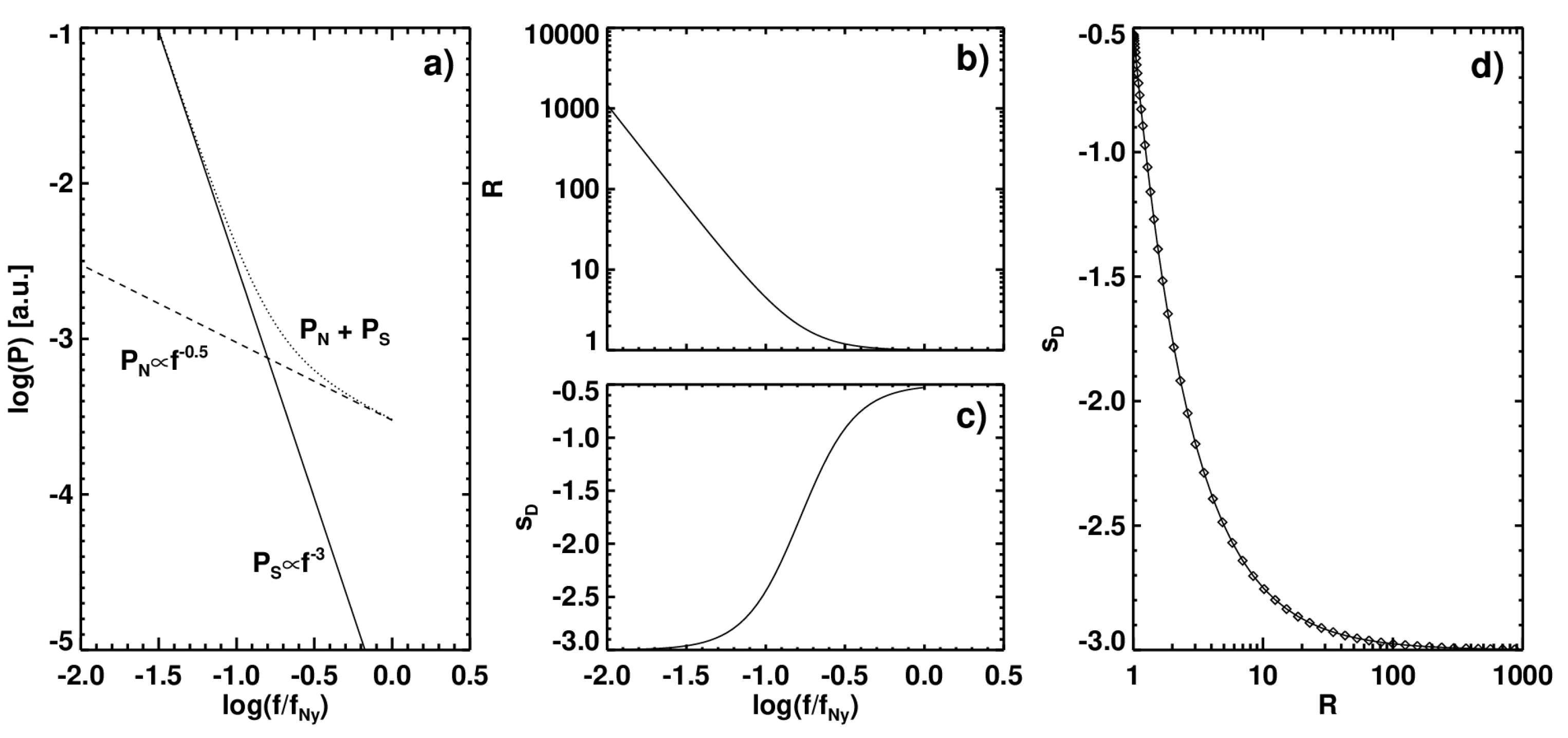
2.1. Signal-to-Noise Ratio

Let us denote the signal, $X_{\mathrm{S}}\left(t\right)$, and the noise, $X_{\mathrm{N}}\left(t\right)$, and their respective power spectra, $P_{\mathrm{S}}$ and $P_{\mathrm{N}}$. The $S/N$ ratio can be defined as the ratio of the power of signal and the power of noise within some frequency band,

$$SNR=\frac{P_{\mathrm{S}}}{P_{\mathrm{N}}}.$$

(1)

We denote the signal sampling rate $\mathsf{\Delta }{x}_{\mathrm{s}}$ and the resulted Nyquist frequency of the signal(noise) $f_{\mathrm{Ny}}=1/\left(2\mathsf{\Delta }{x}_{\mathrm{s}}\right)$. Assuming that both the signal and the noise do not possess any power above $f_{\mathrm{Ny}}$ and are uncorrelated, then the sum $X_{\mathrm{sum}}=X_{\mathrm{S}}+X_{\mathrm{N}}$ satisfies

$$\mathcal{F}\left(X_{\mathrm{sum}}\right)=\mathcal{F}\left(X_{\mathrm{S}}\right)+\mathcal{F}\left(X_{\mathrm{N}}\right),$$

(2)

and therefore,

$$P_{\mathrm{sum}}=P_{\mathrm{S}}+P_{\mathrm{N}},$$

(3)

where $\mathcal{F}$ denotes the Fourier transform and $P_{\mathrm{sum}}$ the sum of the signal and noise powers.

In the framework of this idealized model, we investigate the relationship between the derivative of the power spectra of the signal $P_{\mathrm{S}}$, the noise $P_{\mathrm{N}}$, their sum $P_{\mathrm{sum}}$, and the $SNR$ ratio. We further assume that the power spectra of the signal and noise follow a power law with indices a and b, $P_{\mathrm{S}}\propto f^a$ and $P_{\mathrm{N}}\propto f^b$. Motivated by the frequently adopted approach of analyzing PSDs in a $log\left(f\right)-log\left(P\right)$ coordinate system in many kinetic/MHD range investigations, we carry out the calculation of the derivatives in these coordinates, where power laws are straight lines. Black solid and dashed lines in Figure 1a show two power law functions $P_{\mathrm{S}}\propto f^{-3}$ and $P_{\mathrm{N}}\propto f^{-0.5}$. However, the sum of two power laws is no longer a straight line, but it exhibits a smooth transition between $P_{\mathrm{N}}$ and $P_{\mathrm{S}}$ as shown by the dotted line in the same figure. In the rest of the paper, we use the quantity $R=SNR+1$, instead of $SNR$, because $SNR+1=\frac{P_{\mathrm{S}}+P_{\mathrm{N}}}{P_{\mathrm{N}}}=\frac{P_{\mathrm{sum}}}{P_{\mathrm{N}}}$. We stress that R is defined in the original linear coordinates. We see that the ratio R and the derivative of $P_{\mathrm{sum}}$, $s_{\mathrm{D}}=\frac{\mathrm{d}log{P}_{\mathrm{sum}}}{\mathrm{d}logf}$, depend on the frequency, as is depicted in Figure 1b,c, respectively.

It can be easily shown (see Appendix B) that the following simple equation couples the quantities of interest:

$$s_{\mathrm{D}}=\frac{a(R-1)+b}{R}.$$

(4)

The black solid line in Figure 1d shows the derivative of $P_{\mathrm{sum}}$ as a function of R. Note, that this derivative was estimated independently of Equation (4). If we finitely sample functions $P_{\mathrm{S}}\left(f_i\right)$ and $P_{\mathrm{N}}\left(f_i\right)$ at logarithmically spaced frequencies ($f_{i+1}/f_i=1/8$), we can trivially estimate $P\left(f_i\right)$, $s_{\mathrm{D}}\left(f_i\right)$ and $R\left(f_i\right)$. On the other hand, the black diamonds in Figure 1d were calculated through Equation (4), using $a=-3$ and $b=-0.5$ and $R\left(f_i\right)$, which serve as a visual proof of the equation.

Note that, in practice, we estimate the power $P_{\mathrm{obs}}$ of an observed signal and we estimate $R_{\mathrm{obs}}=P_{\mathrm{obs}}/P_{\mathrm{N}}$, which is not necessarily equal to R, since $P_{\mathrm{obs}}$ may not be equal to a simple sum of the power spectra of the ‘intrinsic’ signal and of the noise.

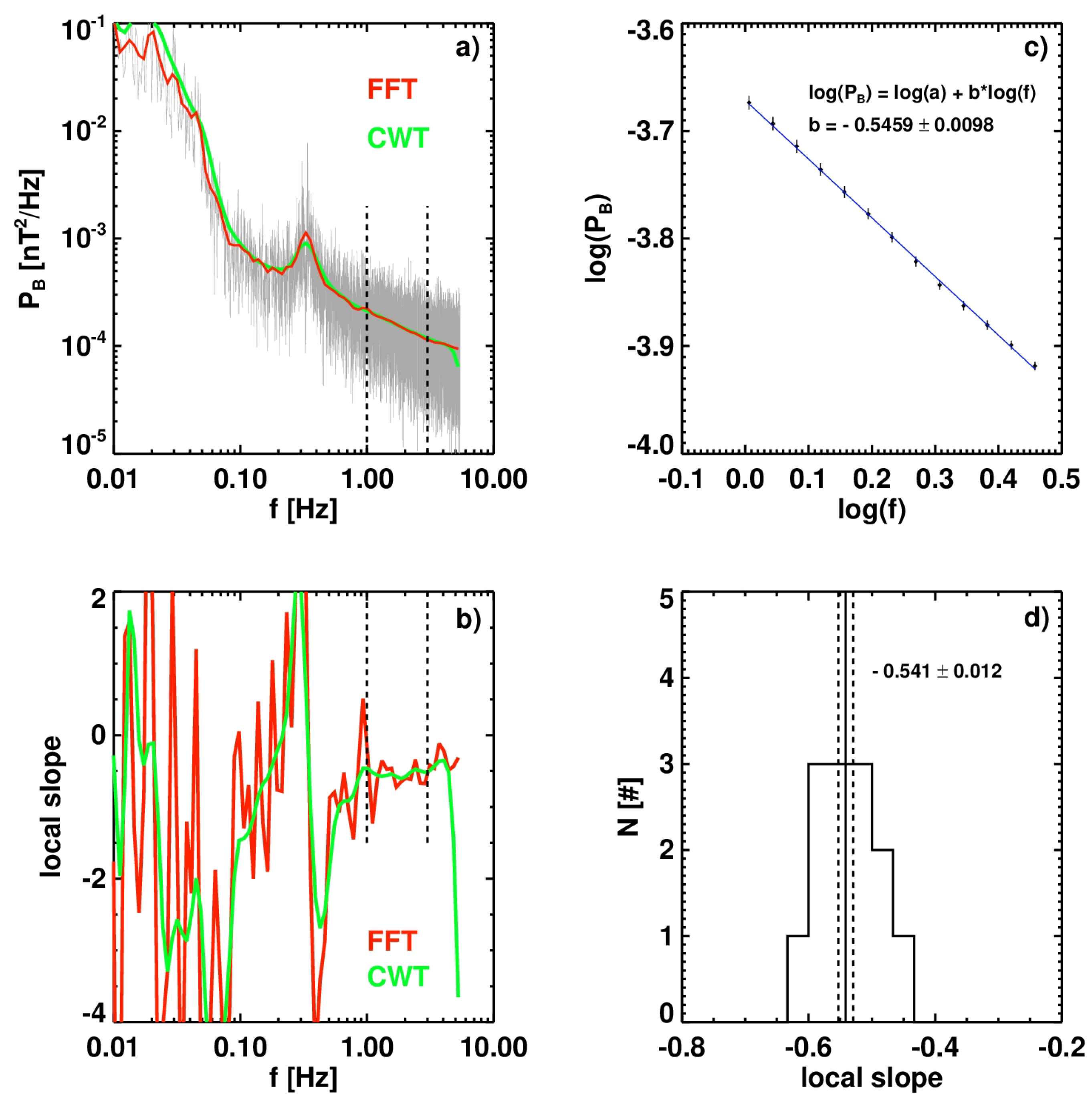
2.2. Continuous Wavelet Transform

Over the past decade, many authors have employed CWT in the computation of spectra of the Interplanetary Magnetic Field (IMF) for example [34,35,36,37]. Due to its optimal frequency and time resolution it is suitable for the analysis of non-stationary signals which are characteristic of MHD and kinetic turbulence. For a discrete set of measurements of one IMF component, $B_z\left(t_i\right)$, which are regularly sampled at $t_i=t_0+i\delta t,$ where $i=0,\cdots ,N-1$ and $\delta t$ is the sampling period, the implementation of wavelet transform reads

$${\mathcal{W}}_z(\tau ,t)=\sum _{i=0}^{N-1}{B}_z\left(t_i\right)\psi \left(\frac{t_i-t}{\tau }\right),$$

(5)

where $\psi$ is the mother wavelet function and $\tau$ is the wavelet scale. A standard choice for the discrete set of values of the scale reads

$${\tau }_j={\tau }_0{2}^{j\delta j},j=0,\cdots ,J,$$

(6)

where $J={\delta j}^{-1}{log}_2(N\delta t/{\tau }_0)$, where $\delta j$ defines the spacing of the consecutive scales. The lowest resolvable scale ${\tau }_0$ is frequently set to $2\delta t$. A Morlet mother function with ${\omega }_0=6$ (for which $f\approx \frac{1}{1.033\tau }$, where f is the equivalent Fourier frequency for any $\tau$ [38]) is usually adopted [34,35,38] and we also use it.

A normalized global wavelet spectrum is defined as the average of the squares of the wavelet coefficients over time,

$$P_{B_z}=\frac{2\delta t}{N}\sum _{i=0}^{N-1}{\left|{\mathcal{W}}_z(\tau ,t_i)\right|}^2.$$

(7)

In the case of a vector quantity, for example, magnetic or velocity fields, the trace PSD is defined as the sum of the power spectra of each component,

$$P_B=P_{B_x}+P_{B_y}+P_{B_z}.$$

(8)

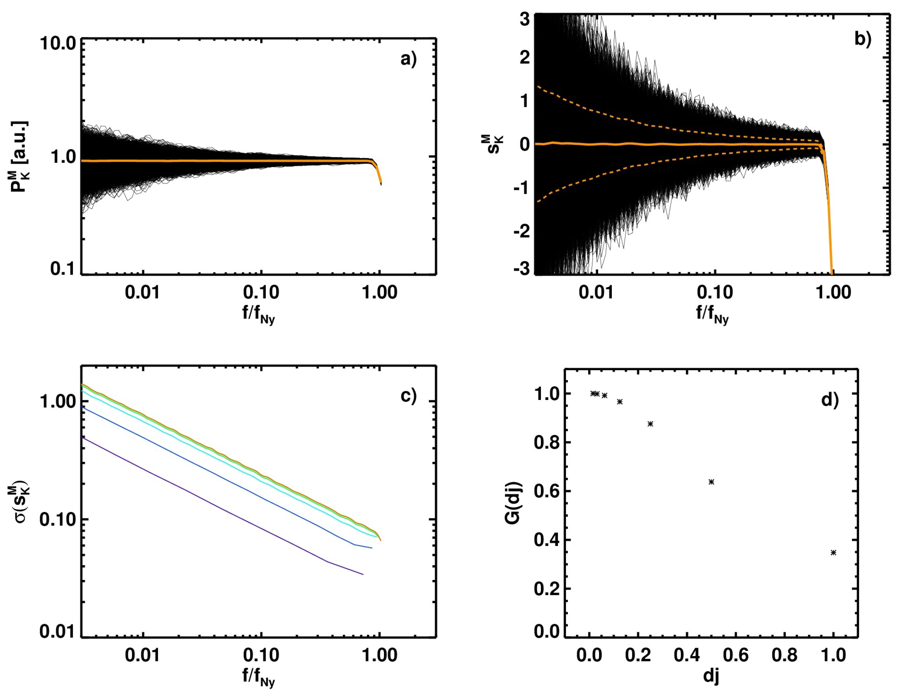
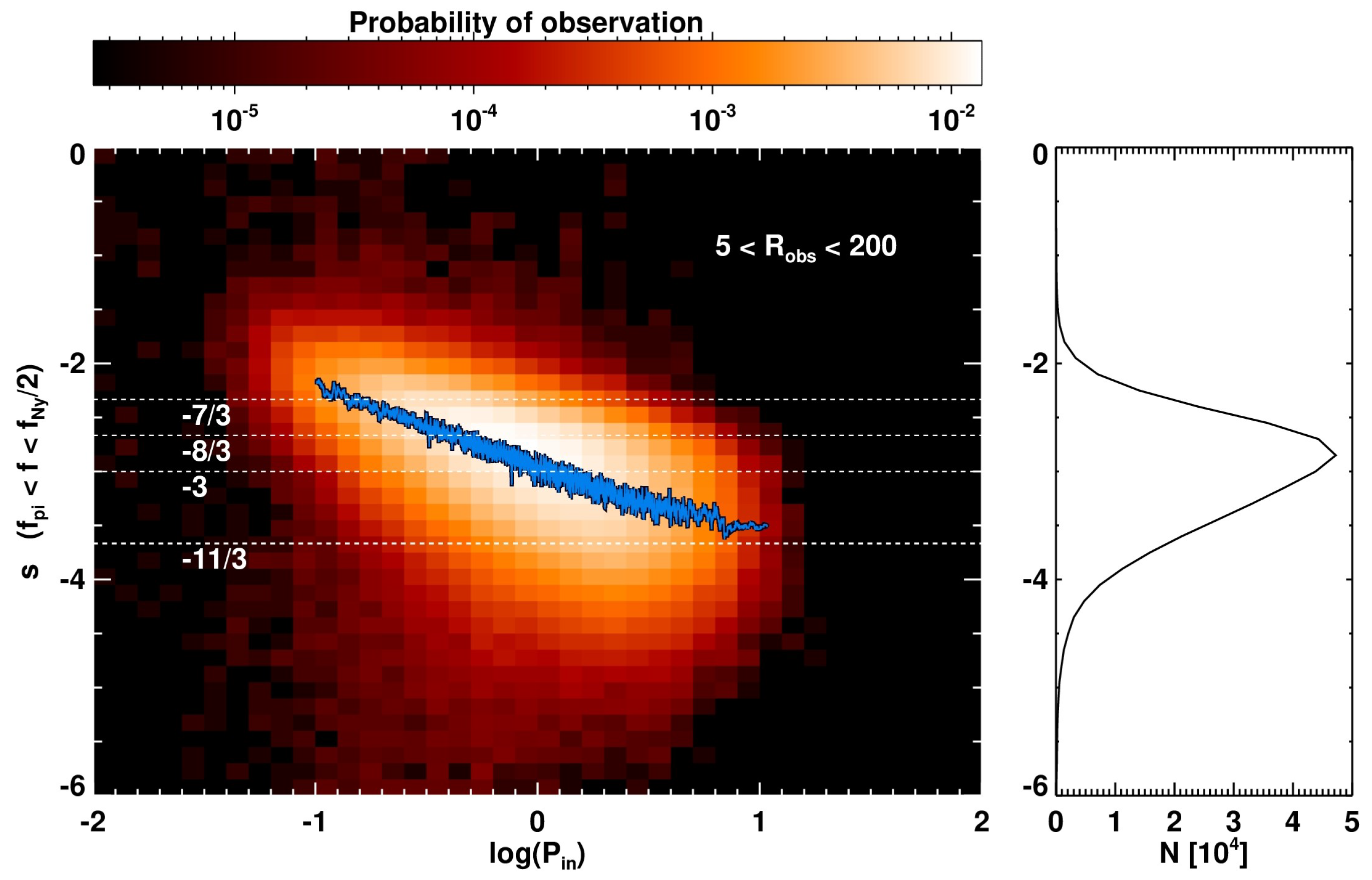
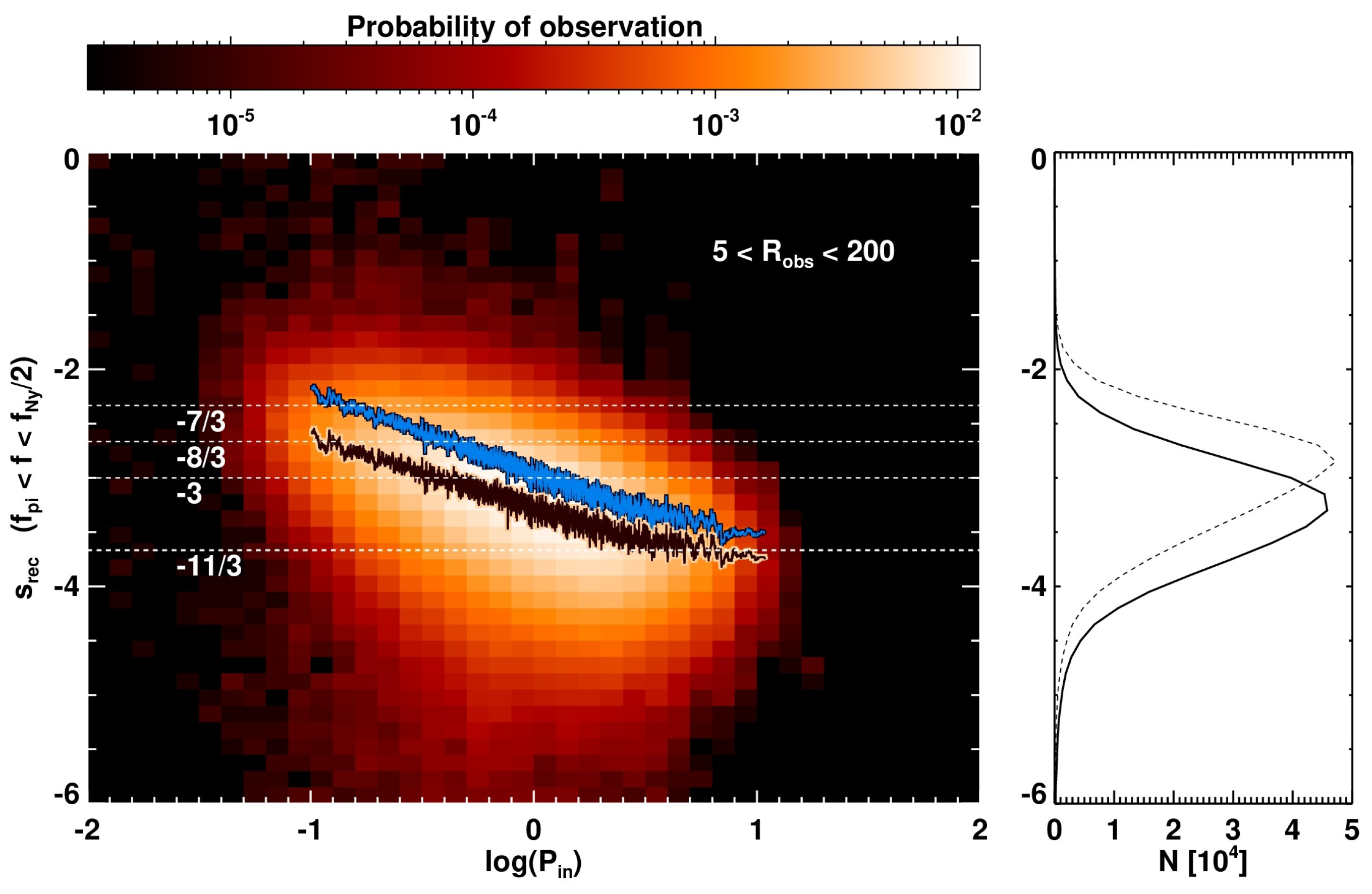
2.3. Local Slope and Monte Carlo Simulations of Its Error Distribution Function

Dudok de Wit et al. [36] argued that estimating power law indices within a short range of frequencies, $(f_{\mathrm{L}}-f_{\mathrm{H}})$, $f_{\mathrm{H}}/f_{\mathrm{L}}<10$, is “extremely risky”. In this section, we undertake this risk and study the most extreme case of power law index estimation: we define a local slope, s, as the ratio of the difference between two consecutive values of global wavelet spectrum and the frequency spacing in a log-log scale,

$$s\left({\tau }_j\right)=\frac{log\left(\frac{P_B\left({\tau }_{j+1}\right)}{P_B\left({\tau }_j\right)}\right)}{log2·\delta j}.$$

(9)

In fact, we are not implicitly assuming a power law behavior within a broader range of frequencies. The advantage of this approach is that no fitting is required and one can examine a broader range of frequencies by simply studying the distribution of the local slopes within the desired range.

Crucial information in any investigation of $s\left({\tau }_j\right)$ is the error of its estimation. Here, instead of a theoretical treatment of this problem, we employ a Monte Carlo technique for the estimation of the error distribution function of $s\left(\tau \right)$. We use an Uncorrelated Multivariate White Noise (UMWN) process and we adopt the following methodology:

(1)

We draw a set of N independent and identically distributed random K-dimensional vectors from ${\mathcal{N}}_K(\mu ,\mathsf{\Sigma })$ (Multivariate normal distribution function with zero mean vector $\mu$ and diagonal covariance matrix $\mathsf{\Sigma }$ with unit variances), denoted as $S_{\mathcal{N}}^K$;

(2)

We estimate the trace power spectral density of $S_{\mathcal{N}}^K$ via CWT (Equations (7) and (8)), $P_K$;

(3)

We repeat (1) and (2) M times to obtain M independent estimations of PSDs, $P_K^M$ (see Figure 2a);

(4)

For each $P_K^M$, we estimate the local slope (Equation (9)) and ($s_K^M\left({\tau }_j\right))$ (see Figure 2b);

(5)

We construct a probability distribution function $\mathcal{A}$ of $s_K^M\left({\tau }_j\right)$ for each scale ${\tau }_j$, ${\mathcal{A}}_K\left({\tau }_j\right)$ and estimate its standard deviation ${\sigma }_s\equiv \sqrt{var\left(s_K^M\left({\tau }_j\right)\right)}$, ${\sigma }_s={\sigma }_s(\tau ,N,\delta j,K)$, where $var$ denotes the variance.

Since the asymptotic PSD ($N\to \infty$) of a band limited white noise is a constant, the derivative of the PSD is 0 in this limit. However, each realization of white noise can only have a finite number of samples N (step one), hence each value of PSD is estimated from a finite set of more or less independent wavelet coefficients which themselves are estimations of a local power in the $t-\tau$ plane [37,38]. Each local slope is thus estimation of its true value. ${\mathcal{A}}_K\left({\tau }_j\right)$ serves as a proxy for their error probability distribution function.

Figure 2c summarizes the results of MC runs for: $M=10,000$, $N=2^{15}$, $K=1$ and $\delta j=\left[2^{-I}\right]$, where $I=0,1,2,\cdots ,6$. The figure shows the standard deviation of the local slope ${\sigma }_s$ as a function of the fraction of the Nyquist frequency for various $\delta j$. We see that each curve in the plot follows a power law $\propto {(f/f_{\mathrm{Ny}})}^{-1/2}$ and that the standard deviation decreases with increasing $\delta j$ for any particular frequency, as it can be expected. When varying the sample size N, we observe the trend ${\sigma }_s\propto N^{-1/2}$ (not shown).

An analytic formula that can be derived from the MC runs reads:

$${\sigma }_s={\mathsf{\Phi }}_{\mathrm{K}}·C_{\mathrm{n}}·N^{-1/2}·{\left(\frac{f}{f_{\mathrm{Ny}}}\right)}^{-1/2}·G\left(\delta j\right),C_{\mathrm{n}}\approx 13.8,$$

(10)

where G is an empirical function depicted in Figure 2d and tabulated in

Table 1. Definition of the function $G\left(\delta j\right)$ (Equation (10)), empirically derived from the MC simulations. Note that we did not estimate $G(\delta j=0)$, but we assigned $G(\delta j=0)\equiv G(\delta j=2^{-6})$. The resulting error of this approximation is negligible since the right-hand derivative of $G(\delta j\approx 0)$ is close to zero.

$\mathit{\delta }\mathit{j}$	$\mathit{G}\left(\mathit{\delta }\mathit{j}\right)$
1/64	1
1/32	0.998
1/16	0.992
1/8	0.966
1/4	0.875
1/2	0.637
1	0.348

, $C_{\mathrm{n}}$ is a normalization constant, N is the number of vectors in one sample, f is the frequency calculated from the wavelet scales ${\tau }_j$, $f_{\mathrm{Ny}}$ is the corresponding Nyquist frequency and ${\mathsf{\Phi }}_{\mathrm{K}}=1/\sqrt{K}$ is a factor that takes into account the dimensionality, K, of the investigated stochastic variable. For a scalar quantity, like the magnitude of the magnetic field, ${\mathsf{\Phi }}_{\mathrm{K}}=1$, while for the magnetic field vector, ${\mathsf{\Phi }}_{\mathrm{K}}=1/\sqrt{3}$.

MC/theoretical treatment of the correlated multivariate white noise (CMWN) is beyond the scope of this paper. However, we introduce a formula for ${\sigma }_s$ that accounts for a special case of CMWN that mimics the magnetic field fluctuations of Alfvénic solar wind turbulence, where the fluctuations perpendicular to the magnetic field are much larger than the parallel ones, $\delta B_{\perp }^2\gg \delta B_{\Vert }^2$. Therefore, the problem is essentially 2D, $K=2$, and the cross-correlations between two perpendicular components with equal variances are parameterized by a correlation coefficient ${\rho }_{\mathrm{comp}}\in \langle -1,1\rangle$. For this special case, we modify Equation (10) with a factor $F_{\mathrm{c}}$:

$${\sigma }_s^{\mathrm{A}}\left(s\right)=F_{\mathrm{c}}·{\mathsf{\Phi }}_{\mathrm{K}}(K=2)·C_{\mathrm{n}}·N^{-1/2}·{\left(\frac{f}{f_{\mathrm{Ny}}}\right)}^{-1/2}·G\left(\delta j\right),F_{\mathrm{c}}=\sqrt{1+{\rho }_{\mathrm{comp}}}.$$

(11)

The correction factor $F_{\mathrm{c}}$ is derived in Appendix C and caveats connected with its application are discussed in Section 4.

3. Statistics of Sub-ion Scale Power Spectra

3.1. Wind MFI and SWE Instruments

For our study of kinetic-range turbulence, we use data from the Wind spacecraft. We take advantage of its nearly continuous measurements of the solar wind plasma. We use high-cadence (0.092 s) data from the Magnetic Field Investigation (MFI) instrument [39,40] and low-cadence (92 s) ion moments from the Solar Wind Experiment (SWE) instrument [41], the proton density, $N_{\mathrm{p}}$, and the solar wind velocity, $V_{\mathrm{sw}}$.

Woodham et al. [33] analyzed the MFI dataset thoroughly and they empirically estimated the “noise floor” of the instrument, that is, they calculated the CWT power spectra of the magnetic field when Wind passed through the tail-lobes of the magnetosphere. They showed that the spectra from different intervals are basically the same in the frequency range of $0.1\mathrm{Hz}<f<5.4\mathrm{Hz}$. They observed a clear peak at $0.33\mathrm{Hz}$, attributed to the spacecraft spin (3 s) [40]. Above this peak, they have found that the noise-floor spectrum can be approximated by a power-law function, $\propto 1.944\times {10}^{-4}{f}^{-0.533}$ resulting from the interplay between the aliasing of the spin tone harmonics and the noise from the digitization process, which shapes the resulted noise-floor PSD.

The MFI instrument can operate in various modes (differing in the final sampling rate-46, 92 or 184 ms) and it has several dynamic ranges. The values when the instrument switches into different ranges are $\pm 4\mathrm{nT}$, $\pm 16\mathrm{nT}$ and $\pm 64\mathrm{nT}$ (up to $\pm 65,536\mathrm{nT}$) and changing the range from, for example, $\pm 16\mathrm{nT}$ to $\pm 64\mathrm{nT}$, should increase the noise level by a factor of 2 [33].

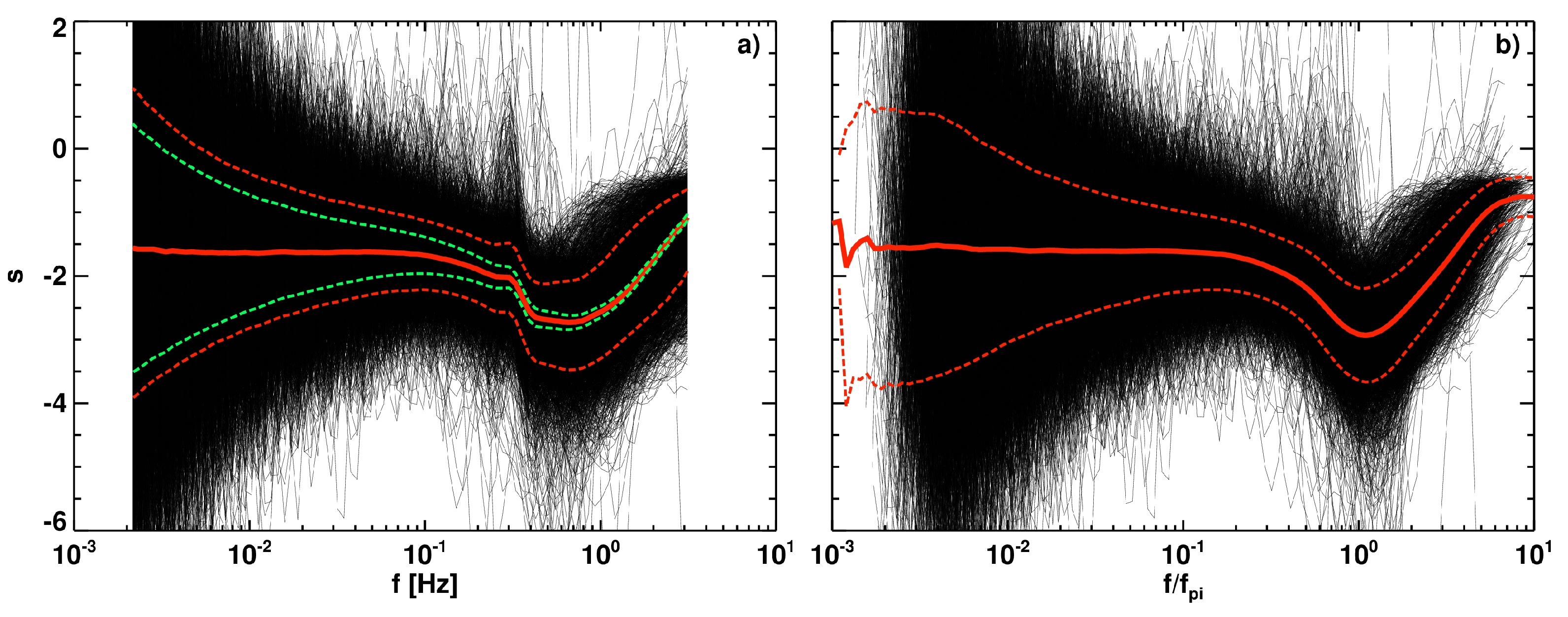
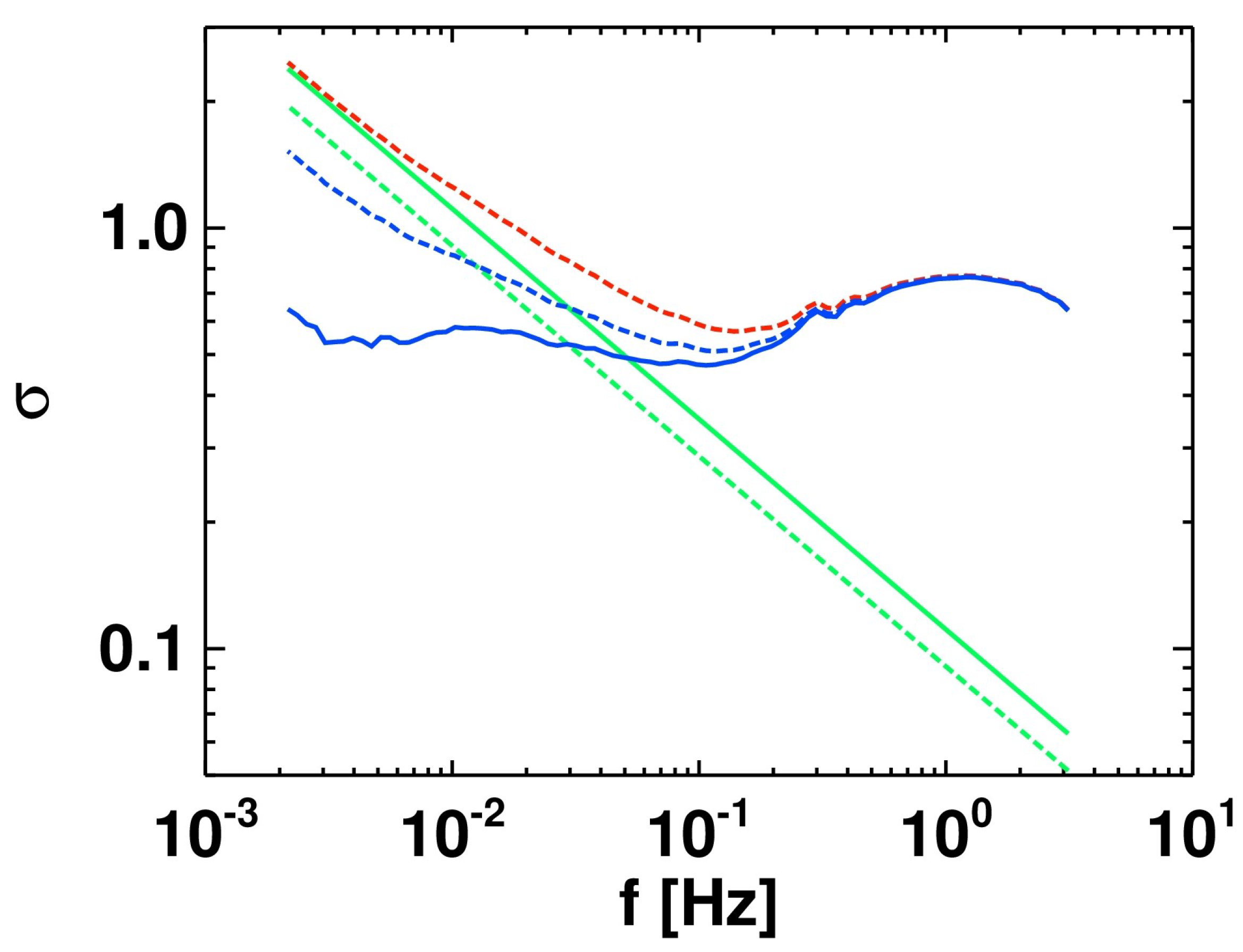
3.2. 11 Years of Wind MFI Data

We analyze 11 years (2006–2016) of MFI Wind data. Within each day, we take 24 non-overlapping one hour intervals, starting from 00:00 UT. The intervals with less than $90\%$ (MFI) and $70\%$ (SWE) data coverage are discarded. Data gaps in the time series of the magnetic field and plasma moments were linearly interpolated. We discarded the intervals which contain Fast Forward (FF) or Fast Reverse (FR) Interplanetary (IP) shocks (Only IP shocks in the Heliospheric Shock Database, generated and maintained at the University of Helsinki (ipshocks.fi) were considered). We use only intervals that were measured in the range $\pm 16\mathrm{nT}$ and did not include range switching. Resulted statistical sample contains 57,895 intervals.

We investigate the kinetic range of magnetic field power spectra in the framework of the simple model introduced in Section 2.1. We estimate PSD via CWT (Equations (7) and (8)) and calculate the local slope using Equation (9). We assume that the noise PSD follows the empirical function reported in [33], denotes as $P_{\mathrm{W}}$ (black line in Figure 3). We clearly see that for the frequencies below ∼0.01 Hz, the supposed noise level is higher than the lowest PSDs in our statistics. As noted by [33], these fluctuations are physical and therefore they should not be considered the ‘true’ noise. However, for those frequencies above ∼0.1 Hz, $P_{\mathrm{W}}$ matches the lowest PSDs in our statistics perfectly.

Since the kinetic range is usually above the spacecraft frame frequency corresponding to the proton inertial length, $f_{\mathrm{pi}}=V_{\mathrm{sw}}/\left(2\pi {\lambda }_{\mathrm{pi}}\right)$, we analyze only PSDs above this frequency. Moreover, we also do not take into account the parts of PSDs near the Nyquist frequency due to a possible enhancement of power due to aliasing [32]. Finally, we analyze only parts of PSDs for $f_{\mathrm{pi}}<f<f_{\mathrm{Ny}}/2$.

Figure 3 shows an overview of all power spectra. The fluctuation power within the inertial range spans roughly four orders of magnitude, while in the kinetic range ($f\simeq 1\mathrm{Hz}$), we clearly see the influence of the noise-floor which limits the range of powers to roughly 1–2 orders of magnitude. For each spectrum, we estimated $f_{\mathrm{pi}}$ and we constructed a blue-colored density map of their positions in the $f-PSDB$ plane. We can see that the peak at 0.33 Hz [40] may significantly influence the local slope values. This influence is demonstrated in Figure 4a, where we plot the local slopes of PSDs for each interval estimated through Equation (9). We see a ‘bump’ in the otherwise smooth transition from inertial to kinetic ranges at ∼0.3 Hz. Furthermore, when looking at the average value (thick red curve), the noise starts to influence the local slope dramatically for frequencies larger than $1\mathrm{Hz}$.

Since many authors use normalization of the spacecraft frame frequencies to Taylor shifted frequencies of some characteristic ion scales for example [19], we show the profiles of local slopes of the PSDs from the upper panel normalized to $f_{\mathrm{pi}}$ in Figure 4b. This panel demonstrates that: (1) although each individual spectrum is influenced by the 0.33 Hz peak, this effect becomes indistinct in the averaged spectrum; and that (2) the local slopes above $f_{\mathrm{pi}}$ are significantly influenced by the noise, on average, implying that any further analysis should consider $S/N$ ratio.

Let us determine the expected error of $s\left(f\right)$ via Equation (10). In our analysis, we have the following set of values: sample size, $N=3600/0.092\approx 39130$, $f_{\mathrm{Ny}}=5.43\mathrm{Hz}$, $\delta j=1/8$, and the dimensionality of B, $K=3$. For the frequencies $0.4\mathrm{Hz}\lesssim f<f_{\mathrm{Ny}}/2$, the calculation yields $0.13\gtrsim {\sigma }_s>0.05$. The green dashed lines in Figure 4a show the profile of ${\sigma }_s$ over the whole range of the investigated frequencies with respect to the median profile (thick red line) of the local slopes. Furthermore, we estimate 1-$\sigma$ deviations of the distribution of the local slopes at each frequency, ${\sigma }_{\mathrm{MFI}}\left(f\right)$. Dashed red lines in Figure 4a show ${\sigma }_{\mathrm{MFI}}$ with respect the median. One can readily see that for $f\gtrsim 1\mathrm{Hz}$, ${\sigma }_{\mathrm{MFI}}\gg {\sigma }_s$ and that for $f\lesssim 0.01\mathrm{Hz}$, ${\sigma }_{\mathrm{MFI}}\gtrsim {\sigma }_s$. Note that, we convincingly recover the frequently reported average slope of B within the inertial range ${\alpha }_{\mathrm{I}}\sim -1.6$.

Next, let us model the distribution of the local slopes $s\left(f\right)$ at any particular frequency f as a PDF of a sum of two uncorrelated random variables. The first being the true local slope, $s_{\mathrm{T}}\left(f\right)$, with the expected value $E\left[s_{\mathrm{T}}\right]\left(f\right)$ given by the solid red line in Figure 4a and with an unknown variance, ${\sigma }_{\mathrm{T}}^2\left(f\right)$. The second being a Gaussian variable with the following PDF: $\mathcal{N}(0,{\sigma }_s^2\left(f\right))$ (gaussian distribution with zero mean and variance given by Equations (10) or (11)). Then we can write:

$${\sigma }_{\mathrm{MFI}}^2={\sigma }_{\mathrm{T}}^2+{\sigma }_s^2.$$

(12)

Since we estimated ${\sigma }_{\mathrm{MFI}}$ and we possess a model for ${\sigma }_s$, we can then estimate ${\sigma }_{\mathrm{T}}$ using Equation (12). Figure 5 summarizes the profiles of ${\sigma }_{\mathrm{MFI}}$ (red dashed line), ${\sigma }_s$ and the resulted ${\sigma }_{\mathrm{T}}$. The dashed and solid green lines show the profile of ${\sigma }_s\left(f\right)$ and ${\sigma }_s^{\mathrm{A}}\left(f\right)$ estimated through Equations (10) and (11), respectively. The dashed and solid blue lines show the corresponding profiles of ${\sigma }_{\mathrm{T}}\left(f\right)$ and ${\sigma }_{\mathrm{T}}^{\mathrm{A}}\left(f\right)$ estimated via Equation (12), assuming ${\sigma }_s\left(f\right)$ and ${\sigma }_s^{\mathrm{A}}\left(f\right)$, respectively. Note that we assumed ${\rho }_{\mathrm{comp}}=0$ in the evaluation of Equation (11). In case of a moderate correlation between the components, ${\rho }_{\mathrm{comp}}\approx 0.5$: ${\sigma }_s^{\mathrm{A}}>{\sigma }_{\mathrm{MFI}}$ and ${\sigma }_{\mathrm{T}}$ would be undefined in the inertial range $f\gtrsim 0.1\mathrm{Hz}$. We discuss this paradox in Section 4.

In the kinetic range, one can see that ${\sigma }_{\mathrm{MFI}}$ results from the variation in the local slope itself, ${\sigma }_{\mathrm{T}}$, rather than from the statistical uncertainty in its estimation ${\sigma }_s$, that is, ${\sigma }_{\mathrm{MFI}}\approx {\sigma }_{\mathrm{T}}>{\sigma }_s$. Furthermore, we stress that ${\sigma }_{\mathrm{T}}^2\left(f\right)$ is not the same as the variance of the intrinsic distribution of the local slopes at frequency f due to the strong influence of the noise floor. The decreasing trend in ${\sigma }_{\mathrm{T}}\left(f\right)$ for $f\gtrsim 1\mathrm{Hz}$ can thus be caused by both (a) decrease of the intrinsic deviation of the local slopes and/or (2) the frequency dependent effect of the noise floor (see Figure 3). We assert that the later effect should be dominant.

On the other hand, the noise should not influence the local slopes well within the inertial range, $2\times {10}^{-3}\mathrm{Hz}<f<2\times {10}^{-2}\mathrm{Hz}$, and therefore, ${\sigma }_{\mathrm{T}}^2$ can be viewed as the intrinsic variation of the local slope. In Figure 5, we can see that, ${\sigma }_{\mathrm{MFI}}$ (dashed red line) and ${\sigma }_s$ (dashed green line) exhibit virtually the same decreasing trend, $\propto f^{-1/2}$, at the lowest frequencies. Moreover, we see that ${\sigma }_{\mathrm{T}}$ (dashed blue curve) in the inertial range is rather large ${\sigma }_{\mathrm{T}}\in \left(1.0,1.5\right)$ and it does not correspond to values reported in previous studies (e.g., Borovsky [27] estimated ${\sigma }_{\mathrm{T}}\approx 0.5$). However, ${\sigma }_{\mathrm{T}}^{\mathrm{A}}$ (solid blue line) exhibits ${\sigma }_{\mathrm{T}}^{\mathrm{A}}\approx 0.6$ in the inertial range. These results show the applicability of Equations (10) and (11) over a wide range of frequencies, surprisingly, even in the inertial range.

Let us now estimate the local slopes above $f_{\mathrm{pi}}$, and their associated $R_{\mathrm{obs}}$ for every interval. We estimate $R_{\mathrm{obs}}$ as the ratio between the $P_B$ and the empirical PSD of the noise level, $P_{\mathrm{W}}$, given by [33]. The resulted distribution of the local slopes and R is depicted in Figure 6. If we identify $R_{\mathrm{obs}}$ with $R_{\mathrm{sum}}$ and s with $s_{\mathrm{D}}$, the distribution follows the trend given by Equation (4): (1) the width of the conditional distribution for any particular value of $R_{\mathrm{obs}}$ is increasing with $R_{\mathrm{obs}}$ and (2) the median trend (black curve) follows the resulted fit (smooth black-and-white curve) of the data by Equation (4) (fitting range $R_{\mathrm{obs}}\in \langle 1.2,100\rangle$). The resulted minimum reduced chi-squared of the fit, ${\chi }_{\mathrm{r},\min }^2\approx 25$, usually imply that the prescribed function models the data poorly, given that the errors in the data are Gaussian and well estimated. However, in our case, the largest factor that causes large ${\chi }_{\mathrm{r},\min }^2$ are the intrinsic variations of the local slope, which act like another source of error. Furthermore, these variations may depend on $R_{\mathrm{obs}}$ and we suspect that they lead to small deviations from the median profile which are present for higher $R_{\mathrm{obs}}$.

When looking at the distribution at low $R_{\mathrm{obs}}$, we see some deviations from the ‘expected’ behavior also. Since the vast majority of the local slopes are estimated over the range of frequencies above the $0.3\mathrm{Hz}$, power spectrum of the noise should scale as $\propto f^{-1/2}$, and therefore it is reasonable to expect that the resulted parameter of the fit ($b_{\mathrm{fit}}=-0.03\pm 0.18$) should be close to $b=-1/2$. Note that for very low levels of $R_{\mathrm{obs}}$, the distribution exhibit a ‘tail’ and it turns towards the value of $-1/2$. We discuss this feature in Section 4.

A natural course of action would be to analyze only the local slopes with high enough $R_{\mathrm{obs}}$, for example, more than 20. On the basis of Figure 1d, the local slope should be underestimated roughly by the same value as its estimated error (${\sigma }_s\sim 0.1$). However, such an approach would introduce a strong bias towards power spectra with high overall levels of fluctuations. On the other hand, if the limiting $R_{\mathrm{obs}}$ will be smaller, the resulted statistics will be biased towards shallower slopes.

We proceed by analyzing the slopes above $R_{\mathrm{obs}}=5$. Motivated by the distribution and the resulting fit in Figure 6, we try to rectify the local slopes using Equation (4) (thus assuming that signal and noise are independent). By keeping the noise slope constant ($b=b_{\mathrm{fit}}=-0.03$), we can compute the asymptotic value ($R_{\mathrm{obs}}\to \infty$) for each local slope, that is, the value of an ‘intrinsic’ local slope that would have been measured in the absence of the noise, $s_{\mathrm{rec}}=a=(s{R}_{\mathrm{obs}}+b)/(R_{\mathrm{obs}}-1)$. Furthermore, a few studies [26,42] showed a dependence of the slopes in the transition range on absolute or relative levels of magnetic field fluctuations, $\delta B$ or $\delta B/B_0$. Let us denote the average $P_B$ within the range of the spacecraft frame frequencies $0.05\mathrm{Hz}<f<0.1\mathrm{Hz}$ as $P_{\mathrm{in}}$. In Figure 7, we show a density plot of the local slope s vs. $P_{\mathrm{in}}$, whereas in Figure 8, a density plot of $s_{\mathrm{rec}}$ vs. $P_{\mathrm{in}}$ is shown (blue line shows the median trend from previous figure). We see that the rectification leads to a steeper local slopes, roughly by ∼0.5 for low $P_{\mathrm{in}}$ and roughly by ∼0.25 for high $P_{\mathrm{in}}$, as it can be expected.

Furthermore, we estimate the error in $s_{\mathrm{rec}}$. We employ the standard formula for error propagation that assumes independent variables, which can be expressed as:

$$var\left(s_{\mathrm{rec}}\right)={\left(\frac{\partial s_{\mathrm{rec}}}{\partial s}\right)}^{2}var\left(s\right)+{\left(\frac{\partial s_{\mathrm{rec}}}{\partial R_{\mathrm{obs}}}\right)}^{2}var\left(R_{\mathrm{obs}}\right)+{\left(\frac{\partial s_{\mathrm{rec}}}{\partial b}\right)}^{2}var\left(b\right).$$

(13)

If we assume that (1) $var\left(s\right)\approx var\left(b\right)$, and (2) $var\left(R_{\mathrm{obs}}\right)\approx var\left(s\right)R_{\mathrm{obs}}^2/18$ (valid for $\delta j=1/8$, see Appendix D for details), after a straightforward evaluation we get:

$$\frac{{\sigma }_{s_{\mathrm{rec}}}}{{\sigma }_s}=\sqrt{\frac{R_{\mathrm{obs}}^2+1}{{\left(R_{\mathrm{obs}}-1\right)}^2}+\frac{R_{\mathrm{obs}}^2}{{\left(R_{\mathrm{obs}}-1\right)}^4}\times \frac{{(b+s)}^2}{18}}.$$

(14)

Since $\left|b+s\right|⪅4$, the first term under the square root dominates the second one for $R_{\mathrm{obs}}\gtrsim 3$ and we can write the final approximation as:

$$\frac{{\sigma }_{s_{\mathrm{rec}}}}{{\sigma }_s}\approx \frac{R_{\mathrm{obs}}}{R_{\mathrm{obs}}-1}.$$

(15)

The dependence of the rectified local slopes on the amplitude/power of the magnetic field fluctuations is qualitatively similar to that of [42]; however, for solar wind intervals exhibiting low levels of fluctuations, we observe significantly steeper slopes (∼−8/3). Interestingly, for high $P_{\mathrm{in}}$, the local slope seems to saturate around $-11/3$, which is a prediction of the current-mediated turbulent regime [43].

4. Discussion and Conclusions

The aim of our study is twofold: (1) we introduce a new way of analyzing the slope of the power spectrum of a physical quantity through the unambiguously defined local slope; and (2) we quantify the effect of an additive noise on the local slope of the spectrum. We illustrate the methods by analyzing the MFI Wind data. In this section, we will discuss the validity of numerous assumptions in the analysis and a few caveats that should be addressed.

Considering the spacecraft data, the assumption of the noise additivity (Equations (2) and (3)) is probably the most questionable. Generally, one would have to prove it or provide a compelling argument that it holds and then proceed with the analysis. Our analysis of the magnetic field fluctuations in Section 3 (Figure 6) convincingly shows that this assumption is in agreement with the empirically estimated distribution of local slopes and signal-to-noise ratios. Note that the assumption does not influence the estimated distribution a priori. Thus, the noise additivity is justified a posteriori.

We hypothesise that the deviations from the expected trend in Figure 6, that is, the ‘tail’ at very low $R_{\mathrm{obs}}$, is caused by the presence of discontinuities within the investigated 1-h intervals. As mentioned above, we discarded the intervals containing the most obvious discontinuities (FF and FR IP shocks). However, we did not attempt to remove the other types (contact, rotational, and tangential discontinuities, slow shocks, etc.). The ‘tail’ of the distribution may be explained in terms of the presence/absence of the discontinuities: for intervals with very low levels of fluctuations (PSD above the 3-Hz peak is virtually at the noise floor) that contain no discontinuities, the estimated local slope is ∼−0.5, while for the intervals that contain discontinuities exhibit enhanced R. Our preliminary analysis showed that if we alter a time series of one MFI Wind interval by introducing a jump, it leads to a non-negligible enhancement of power at all frequencies, whereas the local slope seems to be affected to a lesser extent. Furthermore, the virtual absence of local slopes with $s\gtrsim -0.5$ confirms this suggestion and we may conclude that the whole distribution is on average shifted towards higher $R_{\mathrm{obs}}$. Note that an alternative hypothesis—that the noise level itself is higher by a factor of ∼1.2—cannot be ruled out. However, it is in contrast with the sharp lower bound of the signal-to-noise ratio, $R_{\mathrm{obs}}=1$. We plan to assess the effect of discontinuities in a follow up study.

Furthermore, the obvious bias of the distribution towards lower local slopes for low $R_{\mathrm{obs}}$ in Figure 6 translates into the distribution in Figure 7, that is, the number of local slopes for intervals with higher levels of overall power $P_{\mathrm{in}}$ have a larger contribution in the distribution. This bias cannot be corrected by the rectification procedure, which is used for the calculation of the intrinsic local slope. Therefore, the distribution in Figure 8 is biased towards higher levels of overall fluctuations. In principle, the bias can be corrected if we rectify the whole statistical set, however, that may lead to incorrect results due to: (1) the effects discussed in the previous paragraph; and (2) an enhanced error of the rectified slope approximated by Equation (15). For example, $R_{\mathrm{obs}}=3$ would yield roughly 1.6 enhancement, whereas $R_{\mathrm{obs}}=5$ yields $5/4$ enhancement. With decreasing $R_{\mathrm{obs}}$, the error quickly rises and s has to exhibit unrealistically small errors for a reliable estimation of $s_{\mathrm{rec}}$. The limit $R_{\mathrm{obs}}=5$ used in the analysis of local slopes vs. $P_{\mathrm{in}}$ is rather arbitrary, but it seems to balance the error of resulted intrinsic local slopes and the aforementioned bias towards intervals with higher $P_{\mathrm{in}}$.

Another limitation of our analysis of the transition/kinetic range is a rather small span of the studied frequencies $f_{\mathrm{H}}/f_{\mathrm{L}}\approx \langle f_{\mathrm{pi}}\rangle /\left(3\mathrm{Hz}\right)\approx 5$. The error in the estimation of $f_{\mathrm{pi}}$ should not influence the analysis, since both solar wind speed and density are measured with a good accuracy.

In the MC simulations, we studied a simple uncorrelated multivariate white noise process and we introduced Equation (10), which predicts the standard deviation ${\sigma }_s$ of a local slope s. For a special case of a physically motivated correlated (2D) white noise process, we introduced a correction factor $F_{\mathrm{c}}$ (Equation (11)). In the estimation of the ‘true’ 1-$\sigma$ deviation of the local slope, ${\sigma }_{\mathrm{T}}$ and ${\sigma }_{\mathrm{T}}^{\mathrm{A}}$, we employed both Equations (10) and (11), which yielded unreasonably large or undefined (for reasonable cross-correlations between components, ${\rho }_{\mathrm{comp}}\approx 0.5$) values, respectively. We assume that the reason behind this inconsistency lies in the rather unsubstantiated assumption that the correlations between the components, ${\rho }_{\mathrm{comp}}$, translate into the correlations between their respective power spectra, ${\rho }_P$ (see Appendix C). Indeed, if we imagine a superposition of circularly polarized Alfvén waves, the (linear) correlation between the fluctuating components $B_x$ and $B_y$ would be zero, however, the amplitude of their fluctuations in $P_x$ and $P_y$ would go hand in hand (${\rho }_P>{\rho }_{\mathrm{comp}}\approx 0$). On the other hand, linearly polarized Alfvén waves would exhibit a correlation between both components and their fluctuation powers (${\rho }_P\approx {\rho }_{\mathrm{comp}}$). We conclude that correlation coefficients between magnetic field components do not trivially translate into correlations between their respective powers. Moreover, the condition $\delta B_{\perp }^2\gg \delta B_{\Vert }^2$ is generally satisfied in the inertial range, whereas in the kinetic range, the fluctuations may exhibit significant compressibility $\delta B_{\Vert }^2/\delta B_{\perp }^2\approx 1/2$, the exact value of which depends on the total plasma beta [44]. Therefore, the dimensionality of the problem is no longer $K=2$, and $F_{\mathrm{c}}$ will depend on the cross-correlations of all the three components/powers. We note, however, that the correction factor $F_{\mathrm{c}}$ (Equation (11)) can be as large as $\sqrt{3}$ for $K=3$, and it should not affect the conclusions of the analysis at higher frequencies.

Concerning the validity of our approach to the estimation of the true/intrinsic standard derivation of the local slopes in the inertial range (see Figure 5 and the corresponding analysis), it is important to address the solar wind variability, since it can influence the error estimation ${\sigma }_s^{\mathrm{A}}$. It is reasonable to expect that the slow/fast solar wind may exhibit different values of ${\rho }_P$, therefore, it is likely that ${\sigma }_s^{\mathrm{A}}$ varies for any particular frequency. This may lead to erroneous estimation of ${\sigma }_{\mathrm{T}}^{\mathrm{A}}$. However, for a scalar quantity (magnetic field strength $\left|B\right|$, density, thermal velocity), one can use Equation (10). Unfortunately, the intrinsic fluctuation levels of the magnetic field strength are often around or below the Wind MFI noise floor, which strongly limits the analysis of transitional/kinetic range. Therefore, we do not show the complementary analysis for $\left|B\right|$. However, the estimation of ${\sigma }_{\mathrm{T}}$ for $\left|B\right|$ through Equation (12) yields the value of $\sim 0.8$ in the inertial range.

Under the assumption of a sufficiently sampled process, our technique of local slopes estimated from two subsequent points of the power spectrum leads to the same results as frequently used fitting of the power spectrum over a broader range of frequencies as we demonstrate in Appendix E. For the local slope technique, the power-law behavior can be investigated via the distribution of local slopes and by assessing the error of the local slope estimation. In the inertial range of turbulence, the local slope technique would yield very large errors for any particular interval due to the small statistical sample of the slopes within the desired frequency range (e.g., $f_{\mathrm{H}}/f_{\mathrm{L}}\simeq 10$); however, for the ion or electron scales of solar wind turbulence, our technique may be useful, especially in the presence of an additive noise. However, we should admit that further investigations are necessary to prove the usefulness of the local slope estimation as it was presented here. We plan to address the role of ion plasma beta and inference of various characteristic scales in future studies.

The steepening of the spectra with an enhanced fluctuation level was discussed by Smith et al. [45], Matthaeus et al. [46], and a possible explanation was given in Matthaeus et al. [47]. Larger power indicates a higher cascade rate, and hence larger power in proton kinetic scales. This power dissipates, and therefore less power is left to cascade down to the electron scales. Furthermore, other parameters of the plasma, such as plasma beta [48], ion-to-electron heating rate [49,50] and/or effects of outer scale separation [51] may influence the properties of sub-ion scale cascade. Recent PSP observations [24,26] of a young solar wind suggest that the level normalized cross-helicity (imbalance between the counter-propagating Alfvén wave packets) may play a role in the dynamics of the transitional range, which may lead to the observed steepening. Huang et al. [26] reported a weak anticorrelation between the transition range spectral index and cross-helicity, in relative terms, such a trend is qualitatively consistent with Figure 8 because higher levels of inertial range fluctuations are characteristic for fast solar wind [52], which exhibits non-zero cross-helicity. We plan to address the role of cross-helicity in a future study that will employ hybrid-kinetic simulations and the technique introduced in the current manuscript.

In conclusion, we introduced a novel method of the local slope estimation and explained its utility. We derived the formula that models the error of its estimation in the framework of CWT. We illustrate the versatility of the local slope estimation in the inertial and kinetic range of turbulence by analysing 11 years of MFI Wind magnetic field measurements, where we convincingly show that the trace $P_B$ can be modeled as a sum of an uncorrelated noise and an intrinsic signal. We showed that, for high levels of overall fluctuations, the local slope of the spectra below the scale of the proton inertial length exhibits a scaling compatible with $-11/3$, on average. For lower levels of fluctuations, the average scaling is closer to $-8/3$. Furthermore, we show that the slope of the spectra can be significantly affected even for a signal-to-noise ratio around 10. We believe that the suggested local slope estimation can be employed in an analysis of turbulence around electron scales in the presence of (an additive) noise.

References

1. Iroshnikov, P.S. Turbulence of a Conducting Fluid in a Strong Magnetic Field. Sov. Astron. 1963, 40, 742. [Google Scholar]
2. Kraichnan, R.H. Inertial Range Spectrum of Hydromagnetic Turbulence. Phys. Fluids 1965, 8, 1385–1387. [Google Scholar] [CrossRef] [Green Version]
3. Shebalin, J.V.; Matthaeus, W.H.; Montgomery, D. Anisotropy in MHD turbulence due to a mean magnetic field. J. Plasma Phys. 1983, 29, 525–547. [Google Scholar] [CrossRef] [Green Version]
4. Goldreich, P.; Sridhar, S. Toward a theory of interstellar turbulence. 2: Strong alfvenic turbulence. Astrophys. J. 1995, 438, 763–775. [Google Scholar] [CrossRef]
5. Chen, C.H.K.; Bale, S.D.; Salem, C.S.; Maruca, B.A. Residual Energy Spectrum of Solar Wind Turbulence. Astrophys. J. 2013, 770, 125. [Google Scholar] [CrossRef] [Green Version]
6. Bowen, T.A.; Mallet, A.; Bonnell, J.W.; Bale, S.D. Impact of Residual Energy on Solar Wind Turbulent Spectra. Astrophys. J. 2018, 865, 45. [Google Scholar] [CrossRef] [Green Version]
7. Matthaeus, W.H.; Goldstein, M.L.; Roberts, D.A. Evidence for the presence of quasi-two-dimensional nearly incompressible fluctuations in the solar wind. J. Geophys. Res. 1990, 95, 20673–20683. [Google Scholar] [CrossRef]
8. Dasso, S.; Milano, L.J.; Matthaeus, W.H.; Smith, C.W. Anisotropy in Fast and Slow Solar Wind Fluctuations. Astrophys. J. Lett. 2005, 635, L181–L184. [Google Scholar] [CrossRef]
9. Zank, G.P.; Nakanotani, M.; Zhao, L.L.; Adhikari, L.; Telloni, D. Spectral Anisotropy in 2D plus Slab Magnetohydrodynamic Turbulence in the Solar Wind and Upper Corona. Astrophys. J. 2020, 900, 115. [Google Scholar] [CrossRef]
10. Fu, X.; Li, H.; Guo, F.; Li, X.; Roytershteyn, V. Parametric Decay Instability and Dissipation of Low-frequency Alfvén Waves in Low-beta Turbulent Plasmas. Astrophys. J. 2018, 855, 139. [Google Scholar] [CrossRef] [Green Version]
11. Bowen, T.A.; Badman, S.; Hellinger, P.; Bale, S.D. Parametric Decay of Alfven Waves in the Solar Wind. In Solar Heliospheric and INterplanetary Environment (SHINE 2018); SHINE: Cocoa Beach, FL, USA, 2018; p. 11. [Google Scholar]
12. Chandran, B.D.G. Parametric instability, inverse cascade and the 1/f range of solar-wind turbulence. J. Plasma Phys. 2018, 84, 905840106. [Google Scholar] [CrossRef] [PubMed] [Green Version]
13. Oughton, S.; Matthaeus, W.H. Critical Balance and the Physics of Magnetohydrodynamic Turbulence. Astrophys. J. 2020, 897, 37. [Google Scholar] [CrossRef]
14. Hollweg, J.V. Kinetic Alfvén wave revisited. J. Geophys. Res. 1999, 104, 14811–14820. [Google Scholar] [CrossRef]
15. Howes, G.G.; Cowley, S.C.; Dorland, W.; Hammett, G.W.; Quataert, E.; Schekochihin, A.A. Astrophysical Gyrokinetics: Basic Equations and Linear Theory. Astrophys. J. 2006, 651, 590–614. [Google Scholar] [CrossRef] [Green Version]
16. Schekochihin, A.A.; Cowley, S.C.; Dorland, W.; Hammett, G.W.; Howes, G.G.; Quataert, E.; Tatsuno, T. Astrophysical Gyrokinetics: Kinetic and Fluid Turbulent Cascades in Magnetized Weakly Collisional Plasmas. Astrophys. J. Suppl. Ser. 2009, 182, 310–377. [Google Scholar] [CrossRef] [Green Version]
17. Boldyrev, S.; Horaites, K.; Xia, Q.; Perez, J.C. Toward a Theory of Astrophysical Plasma Turbulence at Subproton Scales. Astrophys. J. 2013, 777, 41. [Google Scholar] [CrossRef] [Green Version]
18. Zhao, J.S.; Voitenko, Y.; Yu, M.Y.; Lu, J.Y.; Wu, D.J. Properties of Short-wavelength Oblique Alfvén and Slow Waves. Astrophys. J. 2014, 793, 107. [Google Scholar] [CrossRef] [Green Version]
19. Chen, C.H.K.; Leung, L.; Boldyrev, S.; Maruca, B.A.; Bale, S.D. Ion-scale spectral break of solar wind turbulence at high and low beta. Geophys. Res. Lett. 2014, 41, 8081–8088. [Google Scholar] [CrossRef] [Green Version]
20. Franci, L.; Landi, S.; Matteini, L.; Verdini, A.; Hellinger, P. Plasma Beta Dependence of the Ion-scale Spectral Break of Solar Wind Turbulence: High-resolution 2D Hybrid Simulations. Astrophys. J. 2016, 833, 91. [Google Scholar] [CrossRef] [Green Version]
21. Safránková, J.; Němeček, Z.; Němec, F.; Přech, L.; Pitňa, A.; Chen, C.H.K.; Zastenker, G.N. Solar Wind Density Spectra around the Ion Spectral Break. Astrophys. J. 2015, 803, 107. [Google Scholar] [CrossRef] [Green Version]
22. Taylor, G.I. The Spectrum of Turbulence. Proc. R. Soc. London. Ser. A-Math. Phys. Sci. 1938, 164, 476–490. [Google Scholar] [CrossRef] [Green Version]
23. Sahraoui, F.; Goldstein, M.L.; Belmont, G.; Canu, P.; Rezeau, L. Three Dimensional Anisotropic k Spectra of Turbulence at Subproton Scales in the Solar Wind. Phys. Rev. Lett. 2010, 105, 131101. [Google Scholar] [CrossRef]
24. Bowen, T.A.; Mallet, A.; Bale, S.D.; Bonnell, J.W.; Case, A.W.; Chandran, B.D.G.; Chasapis, A.; Chen, C.H.K.; Duan, D.; Dudok de Wit, T.; et al. Constraining Ion-Scale Heating and Spectral Energy Transfer in Observations of Plasma Turbulence. Phys. Rev. Lett. 2020, 125, 025102. [Google Scholar] [CrossRef] [PubMed]
25. Duan, D.; He, J.; Bowen, T.A.; Woodham, L.D.; Wang, T.; Chen, C.H.K.; Mallet, A.; Bale, S.D. Anisotropy of Solar Wind Turbulence in the Inner Heliosphere at Kinetic Scales: PSP Observations. Astrophys. J. Lett. 2021, 915, L8. [Google Scholar] [CrossRef]
26. Huang, S.Y.; Sahraoui, F.; Andrés, N.; Hadid, L.Z.; Yuan, Z.G.; He, J.S.; Zhao, J.S.; Galtier, S.; Zhang, J.; Deng, X.H.; et al. The Ion Transition Range of Solar Wind Turbulence in the Inner Heliosphere: Parker Solar Probe Observations. Astrophys. J. Lett. 2021, 909, L7. [Google Scholar] [CrossRef]
27. Borovsky, J.E. The velocity and magnetic field fluctuations of the solar wind at 1 AU: Statistical analysis of Fourier spectra and correlations with plasma properties. J. Geophys. Res. (Space Phys.) 2012, 117, A05104. [Google Scholar] [CrossRef] [Green Version]
28. Alexandrova, O.; Lacombe, C.; Mangeney, A.; Grappin, R.; Maksimovic, M. Solar Wind Turbulent Spectrum at Plasma Kinetic Scales. Astrophys. J. 2012, 760, 121. [Google Scholar] [CrossRef] [Green Version]
29. Sahraoui, F.; Huang, S.Y.; Belmont, G.; Goldstein, M.L.; Rétino, A.; Robert, P.; De Patoul, J. Scaling of the Electron Dissipation Range of Solar Wind Turbulence. Astrophys. J. 2013, 777, 15. [Google Scholar] [CrossRef] [Green Version]
30. Roberts, O.W.; Alexandrova, O.; Kajdič, P.; Turc, L.; Perrone, D.; Escoubet, C.P.; Walsh, A. Variability of the Magnetic Field Power Spectrum in the Solar Wind at Electron Scales. Astrophys. J. 2017, 850, 120. [Google Scholar] [CrossRef]
31. Alexandrova, O.; Jagarlamudi, V.K.; Hellinger, P.; Maksimovic, M.; Shprits, Y.; Mangeney, A. Spectrum of kinetic plasma turbulence at 0.3-0.9 astronomical units from the Sun. Phys. Rev. E 2021, 103, 063202. [Google Scholar] [CrossRef]
32. Russell, C.T. Comments on the Measurement of Power Spectra of the Interplanetary Magnetic Field. In Scientific and Technical Information Office, National Aeronautics and Space Administration; NASA Special Publication: Washington, DC, USA, 1972; Volume 308, p. 365. [Google Scholar]
33. Woodham, L.D.; Wicks, R.T.; Verscharen, D.; Owen, C.J. The Role of Proton Cyclotron Resonance as a Dissipation Mechanism in Solar Wind Turbulence: A Statistical Study at Ion-kinetic Scales. Astrophys. J. 2018, 856, 49. [Google Scholar] [CrossRef]
34. Horbury, T.S.; Forman, M.; Oughton, S. Anisotropic Scaling of Magnetohydrodynamic Turbulence. Phys. Rev. Lett. 2008, 101, 175005. [Google Scholar] [CrossRef] [PubMed] [Green Version]
35. Podesta, J.J. Dependence of Solar-Wind Power Spectra on the Direction of the Local Mean Magnetic Field. Astrophys. J. 2009, 698, 986–999. [Google Scholar] [CrossRef]
36. Dudok de Wit, T.; Alexandrova, O.; Furno, I.; Sorriso-Valvo, L.; Zimbardo, G. Methods for Characterising Microphysical Processes in Plasmas. Space Sci. Rev. 2013, 178, 665–693. [Google Scholar] [CrossRef] [Green Version]
37. Lion, S.; Alexandrova, O.; Zaslavsky, A. Coherent Events and Spectral Shape at Ion Kinetic Scales in the Fast Solar Wind Turbulence. Astrophys. J. 2016, 824, 47. [Google Scholar] [CrossRef] [Green Version]
38. Torrence, C.; Compo, G.P. A Practical Guide to Wavelet Analysis. Bullet. Am. Meteorol. Soc. 1998, 79, 61–78. [Google Scholar] [CrossRef] [Green Version]
39. Lepping, R.P.; Acũna, M.H.; Burlaga, L.F.; Farrell, W.M.; Slavin, J.A.; Schatten, K.H.; Mariani, F.; Ness, N.F.; Neubauer, F.M.; Whang, Y.C.; et al. The Wind Magnetic Field Investigation. Space Sci. Rev. 1995, 71, 207–229. [Google Scholar] [CrossRef]
40. Koval, A.; Szabo, A. Magnetic field turbulence spectra observed by the wind spacecraft. In Solar Wind 13; American Institute of Physics Conference Series; Zank, G.P., Borovsky, J., Bruno, R., Cirtain, J., Cranmer, S., Elliott, H., Giacalone, J., Gonzalez, W., Li, G., Marsch, E., et al., Eds.; AIP: Melville, NY, USA, 2013; Volume 1539, pp. 211–214. [Google Scholar] [CrossRef]
41. Ogilvie, K.W.; Chornay, D.J.; Fritzenreiter, R.J.; Hunsaker, F.; Keller, J.; Lobell, J.; Miller, G.; Scudder, J.D.; Sittler, E.C.J.; Torbert, R.B.; et al. SWE, A Comprehensive Plasma Instrument for the Wind Spacecraft. Space Sci. Rev. 1995, 71, 55–77. [Google Scholar] [CrossRef]
42. Bruno, R.; Trenchi, L.; Telloni, D. Spectral Slope Variation at Proton Scales from Fast to Slow Solar Wind. Astrophys. J. Lett. 2014, 793, L15. [Google Scholar] [CrossRef] [Green Version]
43. Franci, L.; Del Sarto, D.; Papini, E.; Giroul, A.; Stawarz, J.E.; Burgess, D.; Hellinger, P.; Landi, S.; Bale, S.D. Evidence of a “current-mediated” turbulent regime in space and astrophysical plasmas. arXiv 2020, arXiv:2010.05048. [Google Scholar]
44. Matteini, L.; Franci, L.; Alexandrova, O.; Lacombe, C.; Landi, S.; Hellinger, P.; Papini, E.; Verdini, A. Magnetic Field Turbulence in the Solar Wind at Sub-ion Scales: In Situ Observations and Numerical Simulations. Front. Astron. Space Sci. 2020, 7, 83. [Google Scholar] [CrossRef]
45. Smith, C.W.; Hamilton, K.; Vasquez, B.J.; Leamon, R.J. Dependence of the Dissipation Range Spectrum of Interplanetary Magnetic Fluctuationson the Rate of Energy Cascade. Astrophys. J. 2006, 645, L85–L88. [Google Scholar] [CrossRef] [Green Version]
46. Matthaeus, W.H.; Weygand, J.M.; Chuychai, P.; Dasso, S.; Smith, C.W.; Kivelson, M.G. Interplanetary Magnetic Taylor Microscale and Implications for Plasma Dissipation. Astrophys. J. 2008, 678, L141–L144. [Google Scholar] [CrossRef]
47. Matthaeus, W.H.; Parashar, T.N.; Wan, M.; Wu, P. Turbulence and Proton–Electron Heating in Kinetic Plasma. Astrophys. J. Lett. 2016, 827, L7. [Google Scholar] [CrossRef]
48. Schekochihin, A.A.; Kawazura, Y.; Barnes, M.A. Constraints on ion versus electron heating by plasma turbulence at low beta. J. Plasma Phys. 2019, 85, 905850303. [Google Scholar] [CrossRef] [Green Version]
49. Kawazura, Y.; Barnes, M.; Schekochihin, A.A. Thermal disequilibration of ions and electrons by collisionless plasma turbulence. Proc. Natl. Acad. Sci. USA 2019, 116, 771–776. [Google Scholar] [CrossRef] [Green Version]
50. Zhdankin, V.; Uzdensky, D.A.; Werner, G.R.; Begelman, M.C. Electron and Ion Energization in Relativistic Plasma Turbulence. Phys. Rev. Lett. 2019, 122, 055101. [Google Scholar] [CrossRef] [Green Version]
51. Hughes, R.S.; Gary, S.P.; Wang, J. Electron and ion heating by whistler turbulence: Three-dimensional particle-in-cell simulations. Geophys. Res. Lett. 2014, 41, 8681–8687. [Google Scholar] [CrossRef] [Green Version]
52. Pi, G.; Pitňa, A.; Němeček, Z.; Šafránková, J.; Shue, J.H.; Yang, Y.H. Long- and Short-Term Evolutions of Magnetic Field Fluctuations in High-Speed Streams. Solar Phys. 2020, 295, 84. [Google Scholar] [CrossRef]
53. Podesta, J.J. Spectra that behave like power-laws are not necessarily power-laws. Adv. Space Res. 2016, 57, 1127–1132. [Google Scholar] [CrossRef]
Figure 1. We plot (a) the signal and the additive noise, P S and P N , by the solid and dashed black lines, and the resulted sum P sum by a dotted black line, in a log-log scale. (b) R, as a function of frequency. (c) Derivative of P sum , s D , as a function of frequency. (d) Black solid line shows s D as a function of R, while the black diamonds mark the values of s D estimated independently through Equation (4) (using a = 3 and b = 0.5 ) for the finitely sampled R.
Atmosphere 12 01547 g001
Figure 2. Summary plot for a subset of the MC runs; power spectra of M = 10 4 with δ j = 1 / 8 , uncorrelated white noise realizations in a log(P)-log(f) plane (a) and their local slope profiles s ( f ) (b). Thick orange lines show the median values while the dashed orange lines in (b) show the 1- σ deviations from the median. (c) 1- σ deviations of the distribution of s ( f ) as a function of f in a log-log plane with varying δ j ; δ j = 1 (violet), δ j = 0.5 (blue), δ j = 0.25 (turquoise), δ j = 0.125 (green), ⋯, δ j = 2 6 (red). The s ( f ) profiles for δ j = { 2 4 , 2 5 , 2 6 } are indistinguishable. (d) An empirical function G ( δ j ) that accounts for the cross-correlations between the two consecutive values of B in Equation (9).
Atmosphere 12 01547 g002
Figure 3. PSDs of the whole statistical set of 1-h intervals (grey area) and the empirically estimated noise-level-floor of [33] (dashed/solid black line), P W . The dashed part ( f < 0.1 Hz ) signifies the range of frequencies where the estimated noise-floor is influenced by physical fluctuations. The blue 2D histogram shows the distribution of the spacecraft frame frequency corresponding to the proton inertial length and the value of PSD at that frequency for the whole set.
Atmosphere 12 01547 g003
Figure 4. (a) Superposed local slope profiles of PSDs from Figure 3 estimated via Equation (9) with δ j = 1 / 8 (black lines). Thick red curve shows the profile of the median of the local slopes. Dashed red curves mark the central confidence regions that contain 68.3 % of local slopes at each particular frequency f. (b) Superposed local slopes of PSD profiles that have been normalized to k λ pi = f / f pi = 1 . The red curves have the same meaning as in (a). Note that only each 20th PSD (black lines) is actually plotted.
Atmosphere 12 01547 g004
Figure 5. Plot of standard deviations σ MFI , σ s , σ s A , σ T and σ T A as a function of frequency. Red curve shows the profile of σ MFI estimated from the distribution of slopes shown in Figure 4. The dashed and solid green lines mark σ s and σ s A estimated by Equations (10) and (11), respectively. The dashed and solid blue lines show the profiles of σ T and σ T A , respectively, estimated through Equation (12).
Atmosphere 12 01547 g005
Figure 6. Probability of observation of the local slopes above f pi as a function of the signal-to-noise ratio, R obs . The black curve shows the running median over 1000 points and the white smooth curve shows the fit of the data in the range of 1.2 < R obs < 100 with the model given by Equation (4). The embedded plot shows the joint confidence regions for ( a , b ) deduced from the reduced χ 2 function of the fit. The ellipses (from small to large) mark the confidence levels p = { 68.3 % , 95.5 % , 99.7 % } .
Atmosphere 12 01547 g006
Figure 7. Density plot of the local slopes as a function of the average power within the frequency range 0.05 Hz < f < 0.1 Hz . Only the local slopes within 200 > R obs > 5 are included (see Figure 6). Horizontal dashed lines mark the values of theoretically predicted kinetic range power law indices. The blue line shows the running median through 1000 points.
Atmosphere 12 01547 g007
Figure 8. Same density plot as in Figure 7 differing by the method of the local slope estimation: each local slope was rectified through Equation (4) using the parameters a and b from the fit as shown in Figure 6. The black curve shows the running median, while the blue curve shows the running median of the original slope in Figure 7. Solid and dashed black lines on the right plot show the distribution of s rec and the original s from the previous figure, respectively.
Atmosphere 12 01547 g008