Abstract
The monitoring and forecasting of particulate matter (e.g., ) and gaseous pollutants (e.g., NO, , and ) is of significant importance, as they have adverse impacts on human health. However, model performance can easily degrade due to data noises, environmental and other factors. This paper proposes a general solution to analyse how the noise level of measurements and hyperparameters of a Gaussian process model affect the prediction accuracy and uncertainty, with a comparative case study of atmospheric pollutant concentrations prediction in Sheffield, UK, and Peshawar, Pakistan. The Neumann series is exploited to approximate the matrix inverse involved in the Gaussian process approach. This enables us to derive a theoretical relationship between any independent variable (e.g., measurement noise level, hyperparameters of Gaussian process methods), and the uncertainty and accuracy prediction. In addition, it helps us to discover insights on how these independent variables affect the algorithm evidence lower bound. The theoretical results are verified by applying a Gaussian processes approach and its sparse variants to air quality data forecasting.
1. Introduction
It is generally believed that urban areas provide better opportunities in terms of economic, political, and social facilities compared to rural areas. As a result, more and more people are migrating to urban areas. At present, more than fifty percent of people worldwide live in urban areas, and this percentage is increasing with time. This has led to several environmental issues in large cities, such as air pollution [].
Landrigan reported that air pollution caused million deaths worldwide in 2015 []. According to World Health Organization (WHO) statistical data, three million premature deaths were caused by air pollution worldwide in 2012 []. Air pollution has a strong link with dementia, causing 850,000 people to suffer from dementia in the UK []. Children growing up in residential houses near busy roads and junctions have a much higher risk of developing various respiratory diseases, including asthma, due to high levels of air pollution []. Polluted air, especially air with high levels of NO, , and and particulate matter (PM), is considered the most serious environmental risk to public health in urban areas []. Therefore, many national and international organisations are actively working on understanding the behaviour of various air pollutants []. This eventually leads to the development of air quality forecasting models so that people can be alerted in time [].
Essentially, being like a time series, air quality data can be easily processed by models that are capable of time series data processing. For instance, Shen applies an autoregressive moving average (ARMA) model in PM concentration prediction in a few Chinese cities []. Filtering techniques like Kalman filter are also applied to adjust data biases to improve air quality prediction accuracy []. These methods, though with good results reported, are limited by the requirement of a prior model before data processing. Machine learning methods, on the other hand, can learn a model from the data directly. This has enabled them to attract wide attention in recent decades in the field of air quality forecasting. For instance, Lin et al. propose the support vector regression with logarithm preprocessing procedure and immune algorithms (SVRLIA) method, which outperforms general regression neural networks (GRNN) [] and BackPropagation neural networks (BPNN) [] in Taiwan air quality forecasting [].
Recently, inspired by the fact that large scale data are accumulated, deep learning models have been applied in air quality prediction []. Some work has added these deep learning models with the ability to quantify uncertainties introduced by inputs. For instance, Garriga-Alonso et al. endow a deep convolutional network with uncertainty quantification, by taking it as an equivalent of a Gaussian processes (GPs) model []. This is because GPs predictions are accompanied by confidence intervals, which are usually taken as a metric to measure prediction uncertainties. Applications of GPs in air quality forecasting can be found in [,]. However, the involvement of matrix inversion in GPs limits their application in large-scale datasets []. This has inspired research on improving the efficiency of GP models, and a series of efficient GP models have been published []. We also proposed an efficient GP model with application in air quality forecasting []. Despite the rich number of GP models published, there lacks work that investigates how noise level, hyperparameters, etc. affect the performance of GP models. It is necessary because air quality data vary due to seasonal variations and sensor degradations. A well-trained GP model may not work when fed with new data, simply due to measurement noise level change. By knowing how the variation of GPs performance can be attributed to noise level and hyperparameters, etc., we will still be able perform analysis when noise level or hyperparameters vary.
Aiming at this, a general solution is proposed in this paper. It provides insights on how a GP model’s performance is related to measurement noise level and hyperparameters, etc. The main contribution of this work includes (1) a general method for analysing how noise level and hyperparameters of a GP model affect the prediction performance. The variation of the evidence lower bound (ELBO) and the upper bound of the marginal likelihood (UBML) with respect to the noise level and hyperparameters are also given. (2) Neumann series is exploited to approximate the matrix inversion involved in GPs. This helps construct an analytical relation between noise level, hyperparameters, etc., and model performance. (3) A comparative air quality forecasting study between Sheffield, UK, and Pershawar, Pakistan is given, demonstrating that the proposed solution is able to capture how noise level and hyperparameters affect GPs performance.
The remaining part of this paper is as follows. Section 2 provides the theoretical fundamentals involved in this paper; Section 3 elaborates the proposed uncertainty quantification solution. In Section 4, we provide a comparative study of air quality prediction in the same period between the British city Sheffield and Pakistani city Pershawar, and the paper is concluded in Section 5. Appendix A describes the data collection process in Peshawar, Pakistan, and in Sheffield, United Kingdom, and presents maps of the considered areas of these cities. Appendix B gives the World Health Organisation (WHO) criteria for air pollutants. Appendix C gives the approximate derivatives of the GP kernel.
2. Background Knowledge
2.1. Gaussian Processes
Given a set of training data where is the input and is the observation, we can determine a GP model to predict for a new input . For instance, when the output is one-dimensional, the GP model is formulated as
where is the mean function defined as
and is the kernel function [] defined as
where is the additive, independent, identically distributed Gaussian measurement noise with variance , and denotes the mathematical expectation operation.
Given a vector, the n inputs can be aggregated into a matrix , or briefly with the corresponding output vector , or . Similarly, the function values at the test inputs with dimensions of can be denoted as , and we next write the joint distribution of and as
where represents the identity matrix. is the prior covariance matrix of with entry , where is one iff and zero otherwise, and and are column vectors from . The matrix denotes the prior covariance matrix of with entry , where and are column vectors from . The matrices and satisfy , and the entry of the prior covariance matrix of and is , where is a column vector from and is a column vector from .
By deriving the conditional distribution of from (4), where the prior mean is set to be zero for simplicity [], we have the predictive posterior at new inputs as
where
is the prediction at , and
denotes the covariance of .
The hyperparameter incorporated in the mean and covariance functions underpin the predictive performance of GP models, and they are usually estimated by maximising the logarithm of the marginal likelihood
2.2. Neumann Series Approximation
Given a matrix inverse , it can be expanded as the following Neumann series []
which holds if is satisfied. In our case, suppose
where is the main diagonal of and is the hollow. If we substitute in Equation (9) by , we get
which is guaranteed to converge when . We investigated the convergence condition in [], where we proved that if is diagonally dominant, then Neumann series can approximate both fast and accurate. In case is not diagonally dominant, we also provided a way to convert it into a diagonally dominant matrix in [], such that can still be approximated by Neumann series. When Neumann series given in (11) converges, we can then approximate with only the first L terms. The L-term approximation is computed as follows:
For instance, when , we have the approximations
3. Uncertainty Quantification in Gaussian Processes
3.1. Uncertainty in Measurements
It is intuitive that noisy measurements would result in less accurate predictions, just as a poor model would do. However, it is not direct from Equations (6) and (7). We will show in detail how the measurement noise would affect the prediction accuracy.
From Equations (6) and (7), we can see that the measurement noise affects the prediction and the covariance by adding a term to the prior covariance in comparison to the noisy free scenario []. From the way that they originated, we know that both and are symmetrical. Then, a matrix exists such that
where is a diagonal matrix with eigen values of along the diagonal. As a diagonal matrix itself, we have
Therefore, we have the partial derivative of Equation (6) with respect to as
The element-wise form of Equation (16) can be therefore obtained as
where . and are the entries indexed by the j-th column, h-th and i-th row, respectively. is the o-th row and h-th column entry of . is the i-th element of . denotes the o-th element of the partial derivation.
We can see that the sign of Equation (17) is determined by and . This is because we can actually transform to either positive or negative with a linear transformation, which will not be an issue for the GPs model. When we impose no constraints on and , Equation (17) could be any real number, indicating that is multimodal with respect to , which means that one can lead to different , or equivalently, different can lead to the same . In such cases, it is difficult to investigate how affects the prediction accuracy. In this paper, to facilitate the study of the monotonicity of , we constrain and to satisfy
Then, we can see that is monotonic. It means that changes of can cause arbitrarily large/small predictions, whereas a robust method should bound the prediction errors regardless of how varies.
Similarly, the partial derivative of Equation (7) with respect to is
where we denote the dimension matrix as
with a vector, and .
As the uncertainty is indicated by the diagonal elements, we only show how these elements change with respect to . The diagonal elements are given as
with denoting the diagonal elements of a matrix. We see that stands for , which implies that is non-decreasing as increases. This means that the increase of measurement noise level would cause the non-deceasing of the prediction uncertainty.
3.2. Uncertainty in Hyperparameters
Another factor that affects the prediction of a GPs model is the hyperparameters. In Gaussian processes, the posterior, as shown in Equation (5), is used to do the prediction, while the marginal likelihood is used for hyperparameters selection []. The log marginal likelihood as shown in Equation (22) is usually optimised to determine the hyperparameter with a specified kernel function.
However, the log marginal likelihood could be non-convex with respect to the hyperparameters, which implies that the optimisation may not converge to the global maxima []. A common solution dealing with it is to sample multiple starting points from a prior distribution, then choose the best set of hyperparameters according to the optima of the log marginal likelihood. Let’s assume being the hyperparameter set and denoting the s-th of them, then the derivative of with respect to is
where , and denotes the trace of a matrix. The derivative in Equation (23) is often multimodal and that is why a fare few initialisations are used when conducting convex optimisation. Chen et al. show that the optimisation process with various initialisations can result in different hyperparameters []. Nevertheless, the performance (prediction accuracy) with regard to the standardised root mean square error does not change much. However, the authors do not show how the variation of hyperparameters affects the prediction uncertainty [].
An intuitive explanation to the fact of different hyperparameters resulting with similar predictions is that the prediction shown in Equation (6) is non-monotonic itself with respect to hyperparameters. To demonstrate this, a direct way is to see how the derivative of (6) with respect to any hyperparameter changes, and ultimately how it affects the prediction accuracy and uncertainty. The derivatives of and of are as below
We can see that Equations (24) and (25) are both involved with calculating , which becomes enormously complex when the dimension increases. In this paper, we focus on investigating how hyperparameters affect the predictive accuracy and uncertainty in general. Therefore, we use the Neumann series to approximate the inverse [].
3.3. Derivatives Approximation with Neumann Series
The approximation accuracy and computationally complexity of Neumann series varies with L. This has been studied in [,], as well as in our previous work []. This paper aims at providing a way to quantify uncertainties involved in GPs. We therefore choose the 2-term approximation as an example to carry out the derivations. By substituting the 2-term approximation into Equations (24) and (25), we have
Due to the simple structure of matrices and , we can get the element-wise form of Equation (26) as
Similarly, the element-wise form of Equation (27) is
where denotes the o-th output, is the j-th row and i-th column entry of , and are the o-th row, j-th and i-th entries of matrix , respectively. When the kernel function is determined, Equations (26)–(29) can be used for GPs uncertainty quantification.
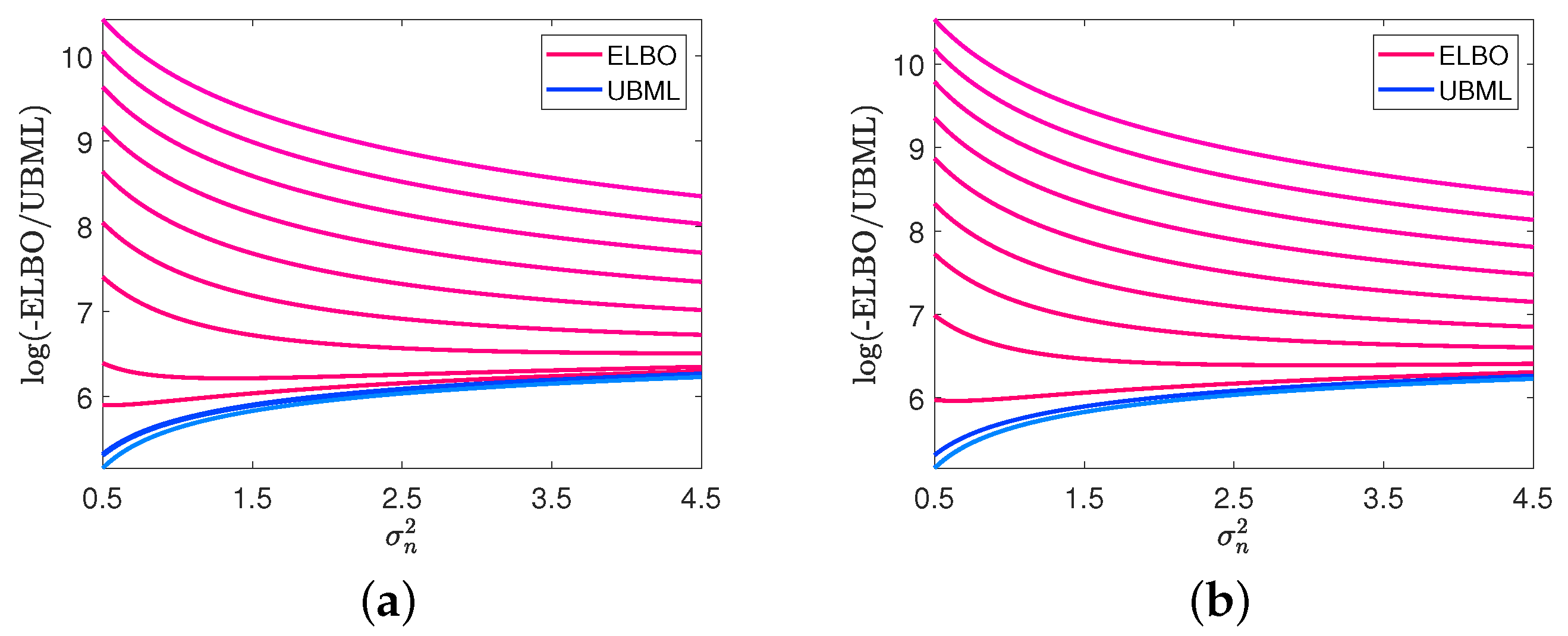
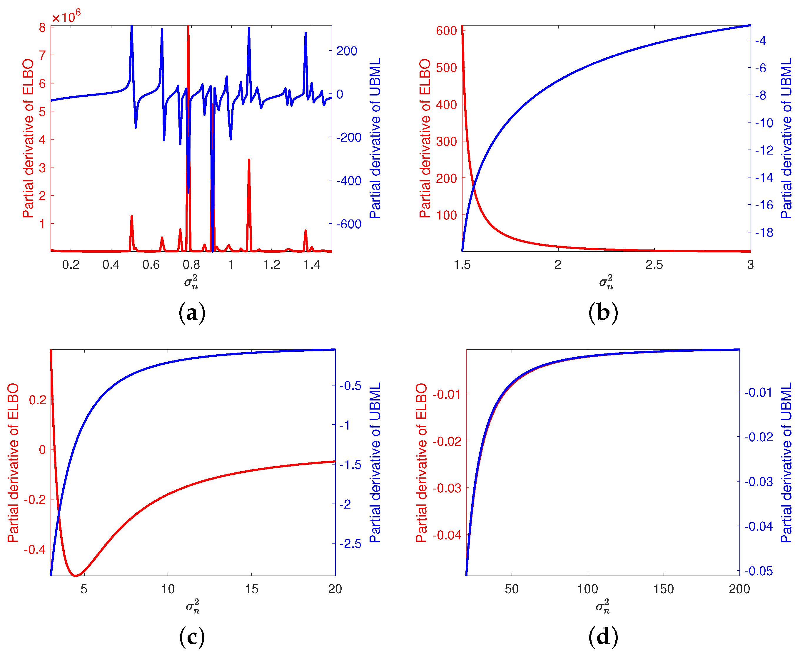
3.4. Impacts of Noise Level and Hyperparameters on ELBO and UBML
The minimisation of is equivalent to maximise the ELBO [,] as shown in
where , and . Combining it with UBML, as shown in Equation (31), an interval can be given to quantify the uncertainty in marginal likelihood.
This paper, however, focuses on investigating how ELBO and UBML change according to only. Because the investigation of how ELBO and UBML change with respect to kernel hyperparameters involves multiple Neumann series approximations, which makes the analysis less convincing. We shall leave it as an open problem for future study. The derivatives of Equations (30) and (31) with respect to are as follows,
Figure 1 shows how affects ELBO and UBML. We set to increase from 0.1 to 200.0 with a step of 0.01. Both ELBO and UBML are recorded step by step. From the figure, we can see that when is small (), ELBO increases with different speeds, however, UBML fluctuates as the derivative of UBML jumps between positive and negative. When is in [1.5, 3.0], ELBO still increases, but the speeds slow down significantly. In comparison, UBML keeps decreasing with reducing speeds. The decrements of UBML mean that when increases, though ELBO could be increased still, but the maximum (which is the UBML) can decrease. When , ELBO starts to decrease when , while UBML keeps decreasing. This means that as increases, both ELBO and UBML decrease, which indicates that the model becomes less and less effective to explain the data. When keeps increasing (), the decreasing speeds of ELBO and UBML becomes similar and approaches zero. This means that UBML and ELBO both converge and together define an interval for the marginal likelihood, which however, can result in non-optimal hyperparameters. Our conclusion is that when increases, UBML tends to decrease, which decreases the maximum that ELBO can reach. ELBO, on the other hand, is robust to the change of (as it keeps increasing when is below ∼3.2). However, when exceeds a certain threshold, ELBO turns to decrease, indicating that the GPs model becomes less and less reliable. However, both ELBO and UBML converge, even when becomes very significant, though we can no longer trust the model.
Figure 1.
Impacts of on ELBO and UBML: (a) , (b) , (c) , (d) .
4. Experiments and Analysis
To verify that the proposed solution can help to identify the impacts of and on the predition accuracy and uncertainty of GPs model and its sparse variants such as the fully independent training conditional (FITC) [] and variational free energy (VFE) [] models, we conduct various experiments to process air quality data collected from Sheffield, UK, and Pershawar, Pakistan (see Appendix A), during the time period of 24 June 2019–14 July 2019 for three weeks, which will be denoted as W1, W2, and W3 hereafter. The data were collected with digital sensors called AQMesh pod with a 15 min time interval. Though the sensor itself is able to measure the concentrations of quite a few atmospheric pollutants, here we only analyse the concentrations of NO, NO, SO, and PM. Figure 2 shows the raw data. We can see directly that the air quality of Sheffield is much better than Pershawar on average. Especially during daytime, concentrations of NO and PM in Pershawar exceed the WHO criteria (see Appendix B). Meanwhile, those in Sheffield are much lower than the criteria. Being a postindustrial city itself, Sheffield has improved air quality significantly. The experience can be spread to help cities like Pershwar to improve air quality.
Figure 2.
Concentration of pollutants recorded at the same time period in both Sheffield and Peshawar: (a) NO, (b) , (c) , (d) .
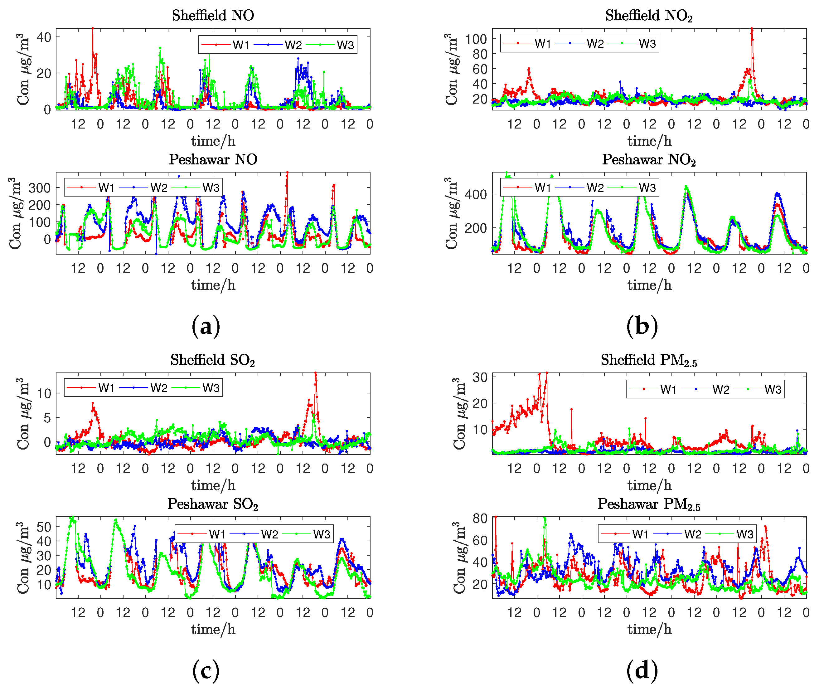
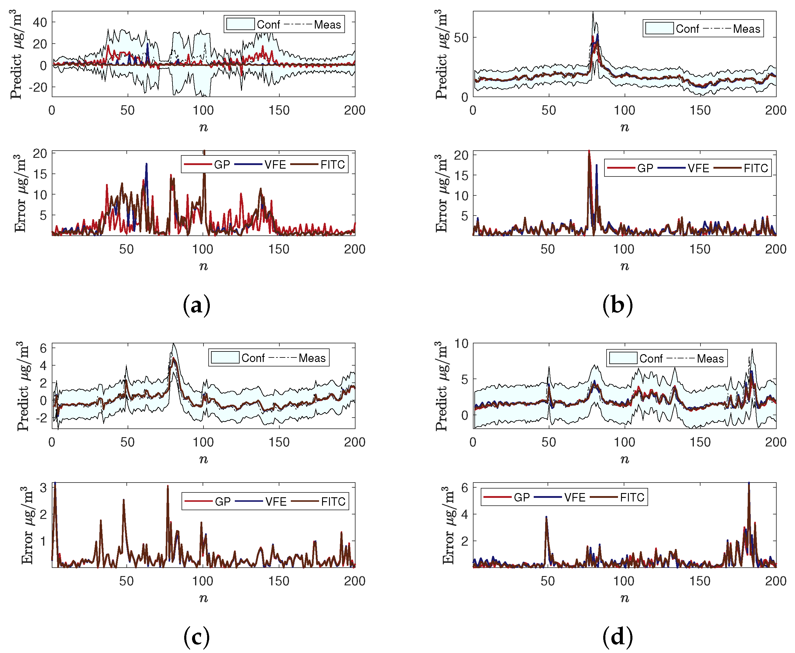
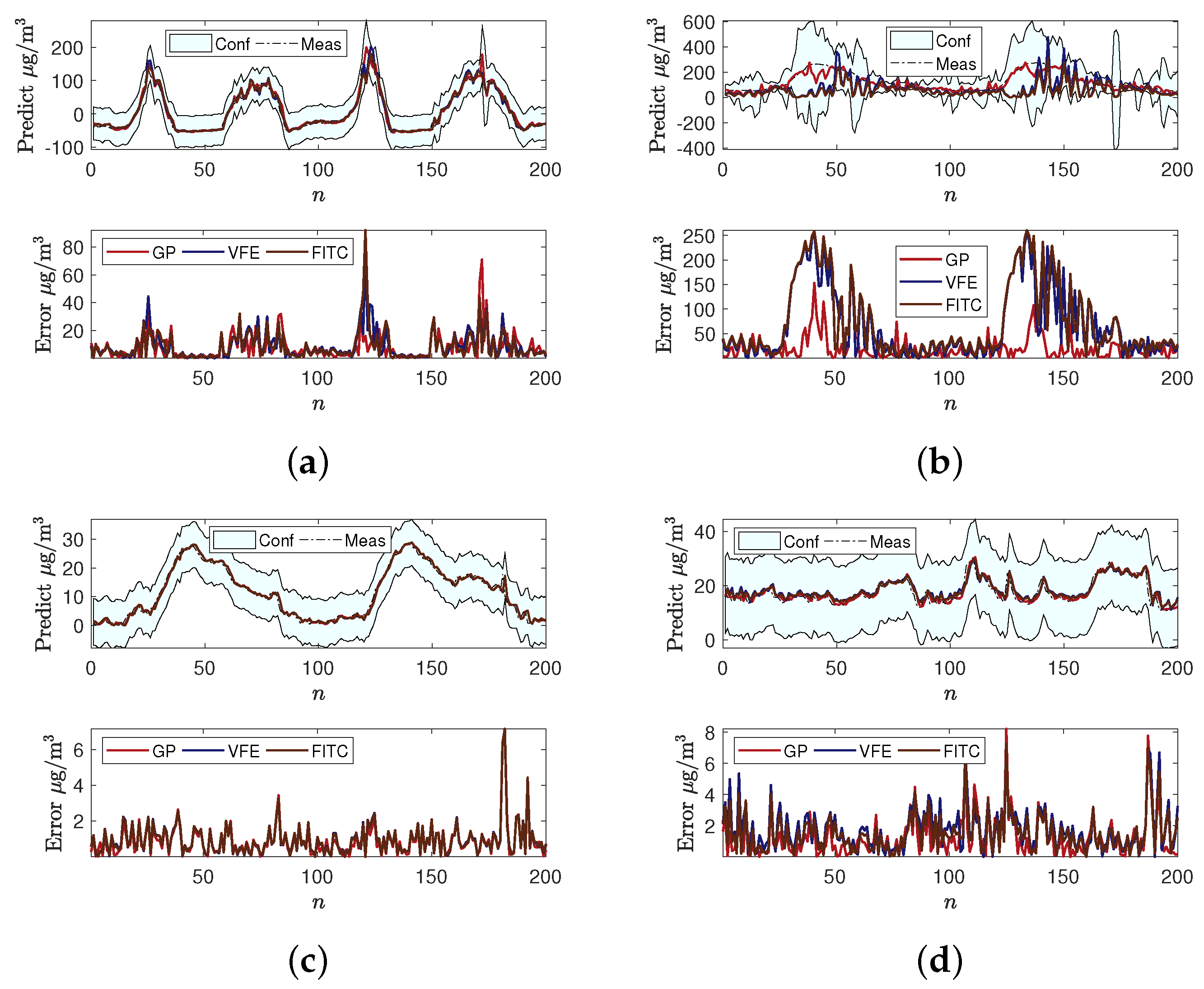
4.1. Air Quality Prediction
Figure 3 and Figure 4 show Sheffield and Pershawar forecasting results of GPs, FITC, and VFE, with confidence intervals (denoted as Conf in the figures) indicated by the shaded area. We can see that the GPs model reports the best results in general, in terms of absolute error between predicts and measurements (denoted as Meas in the figures). However, the performance of all the models varies from pollutant types to cities. This is actually one of the reasons why the investigation of how measurement noise level and hyperparameters affect prediction accuracy and uncertainty is necessary. To make the results more convincing, we normalise the data from both cities for uncertainty quantification studies.
Figure 3.
Prediction and absolute error of pollutants in Sheffield: (a) NO, (b) , (c) , (d) .
Figure 4.
Prediction and absolute error of pollutants in Peshawar: (a) NO, (b) , (c) , (d) .
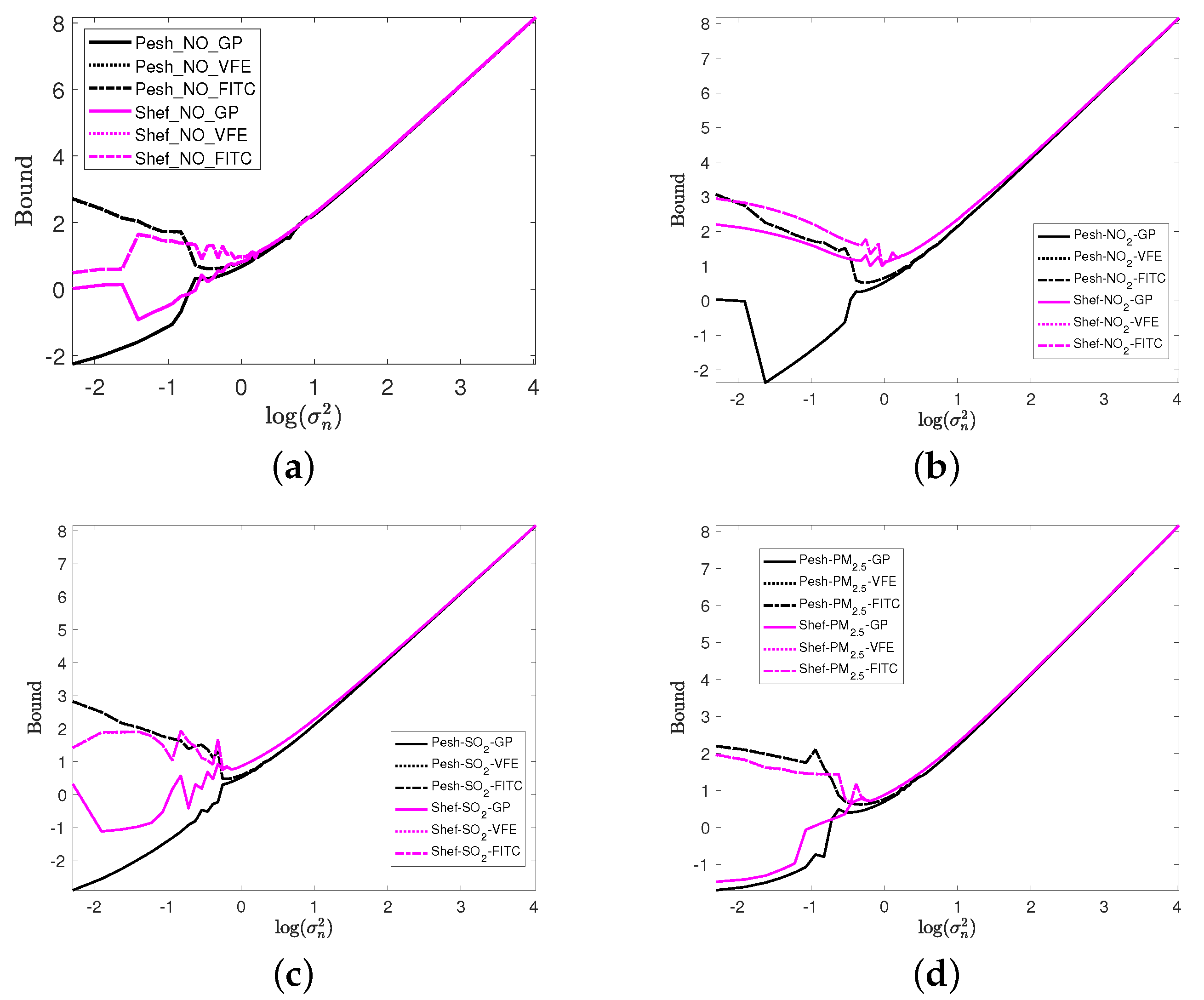
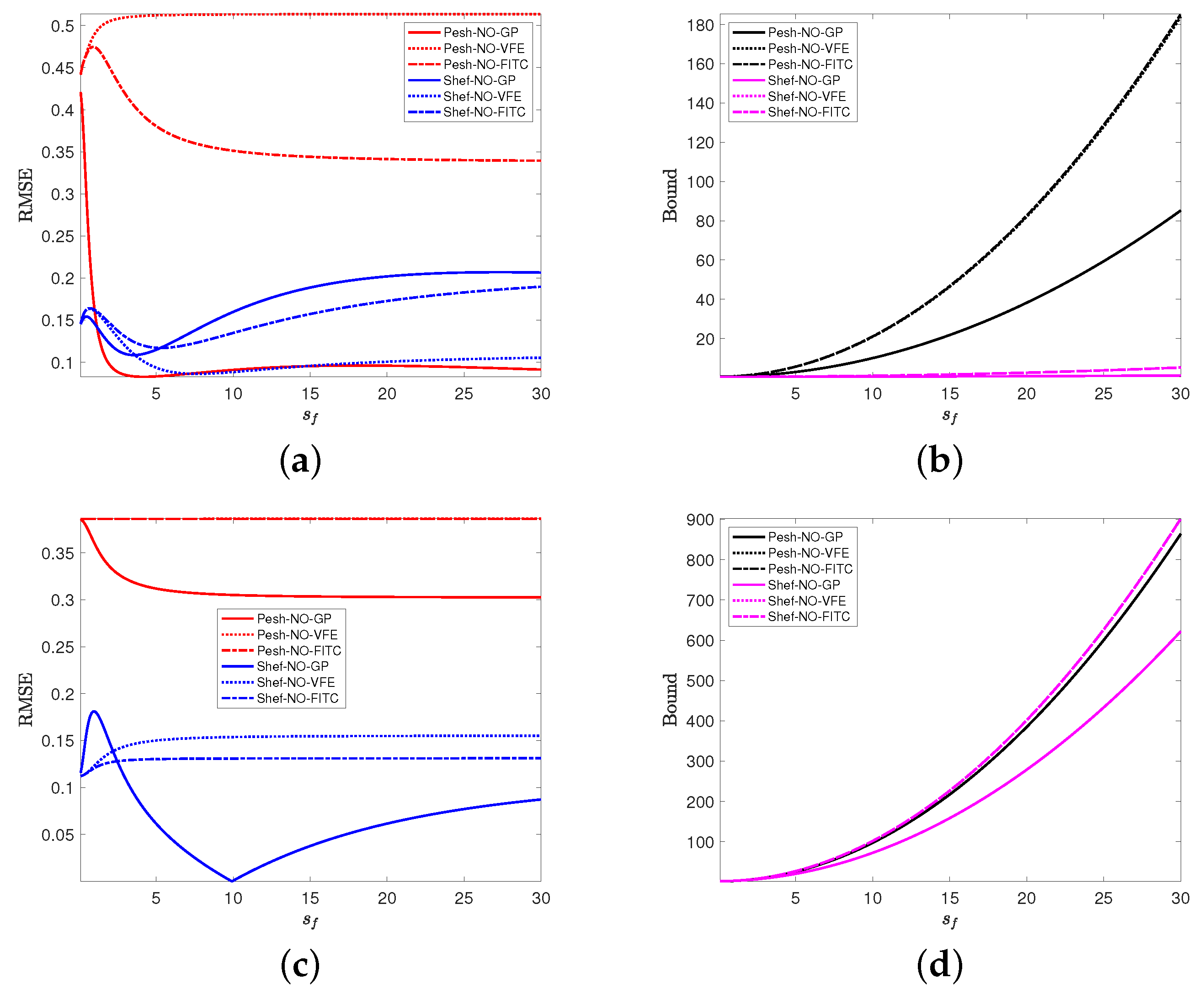
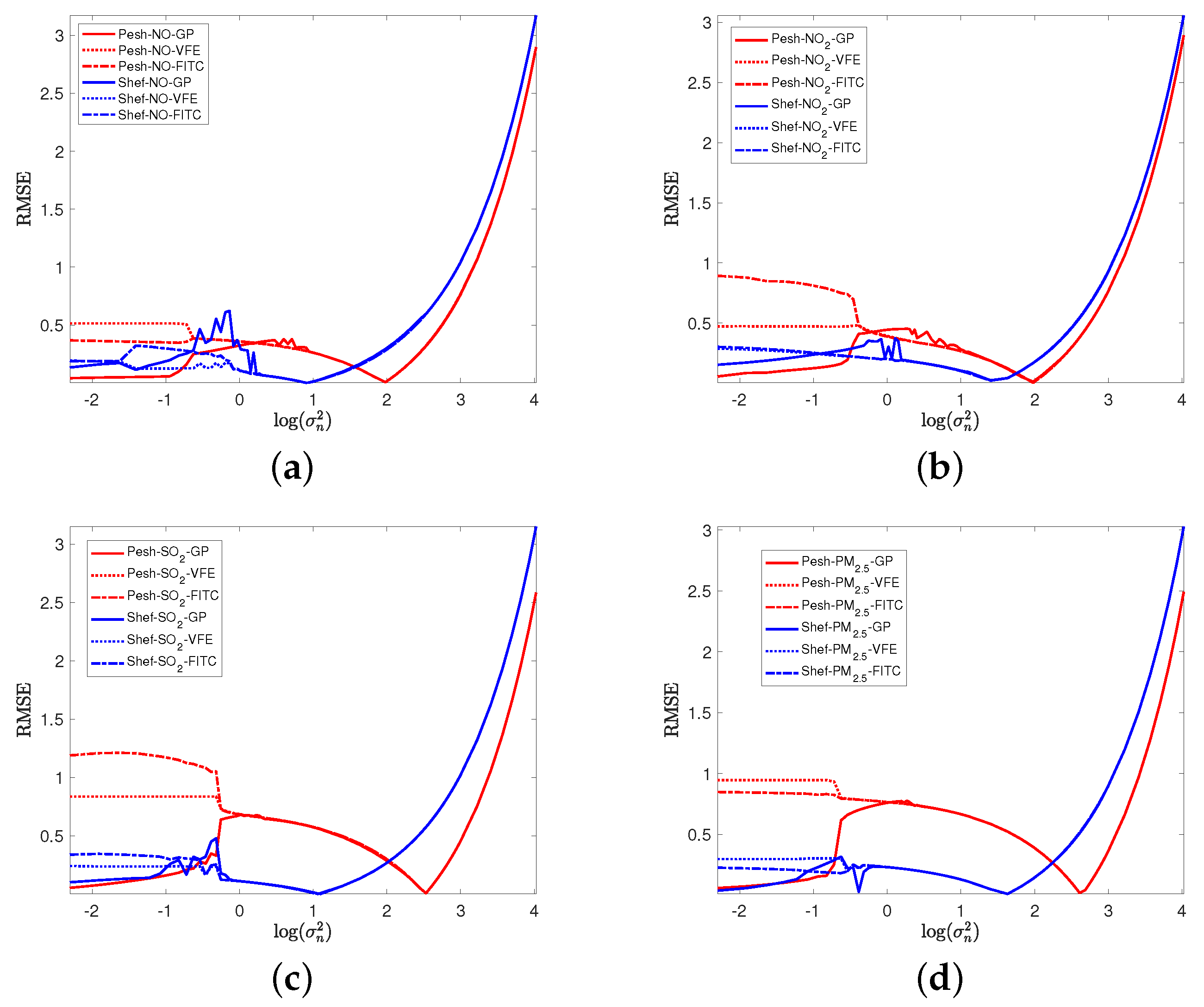
4.2. Impacts of Measurement Noise Level and Hyperparameters
To demonstrate how noise level and hyperparameters affect prediction accuracy and uncertainty, three sets of experiments are conducted. This paper adopts the squared exponential (SE) kernel, with hyperparameters and l. The analytical derivation can be found in Appendix C. The prediction accuracy is identified by the root mean square error (RMSE), as shown in Equation (34), while the uncertainty is identified by confidence bound. Configurations of the experiments are as follows.
Experiment 1: Impacts of on prediction accuracy and uncertainty. Both and l are fixed to be the optimised values. varies from 0.1 through to 20.0. NO, , , and data from both cities are processed. Six inducing points are applied to both FITC and VFE.
Experiment 2: Impacts of on prediction accuracy and uncertainty. l is set to the optimised value. varies from 0.1 through to 30.0. is set to 0.5 and 1.5, respectively. NO data from both cities are processed. Six inducing points are applied to both FITC and VFE.
Experiment 3: Impacts of l on prediction accuracy and uncertainty. is set to the optimised value. l varies from 0.1 through to 30.0. is set to 0.5 and 1.5, respectively. NO data from both cities are processed. Six inducing points are applied to both FITC and VFE.
where is the ground truth value and represents predicted meant. is the sample number in testing set.
Figure 5 and Figure 6 show the results from Experiment 1. To make the results more distinguishable, the horizontal axes of the figures are set to . We can see from Figure 5 that when is small, GPs perform the best in general, while the performance of FITC and VFE varies. We can also observe that as keeps increasing, the RMSE becomes very significant for all methods/pollutants. Similar results can be observed from Figure 6 as well. Both comply with our theoretical conclusions, despite the fact that the Neumann series is used to approximate the matrix inverse. We also notice that has a more significant impact on Sheffield data as RMSE increases ealier after reaches zero. From Figure 6b,c, we also see that the uncertainty bounds of Sheffield data are greater after reaches zero. We think the reason is that Sheffield data are generally less periodical than Pershawar data (see Figure 2), which influences the performance of the models.
Figure 5.
Relationship of with four pollutants prediction RMSE: (a) NO, (b) , (c) , (d) .
Figure 6.
Relationship of with pollutants prediction uncertainty bound: (a) NO, (b) , (c) , (d) .
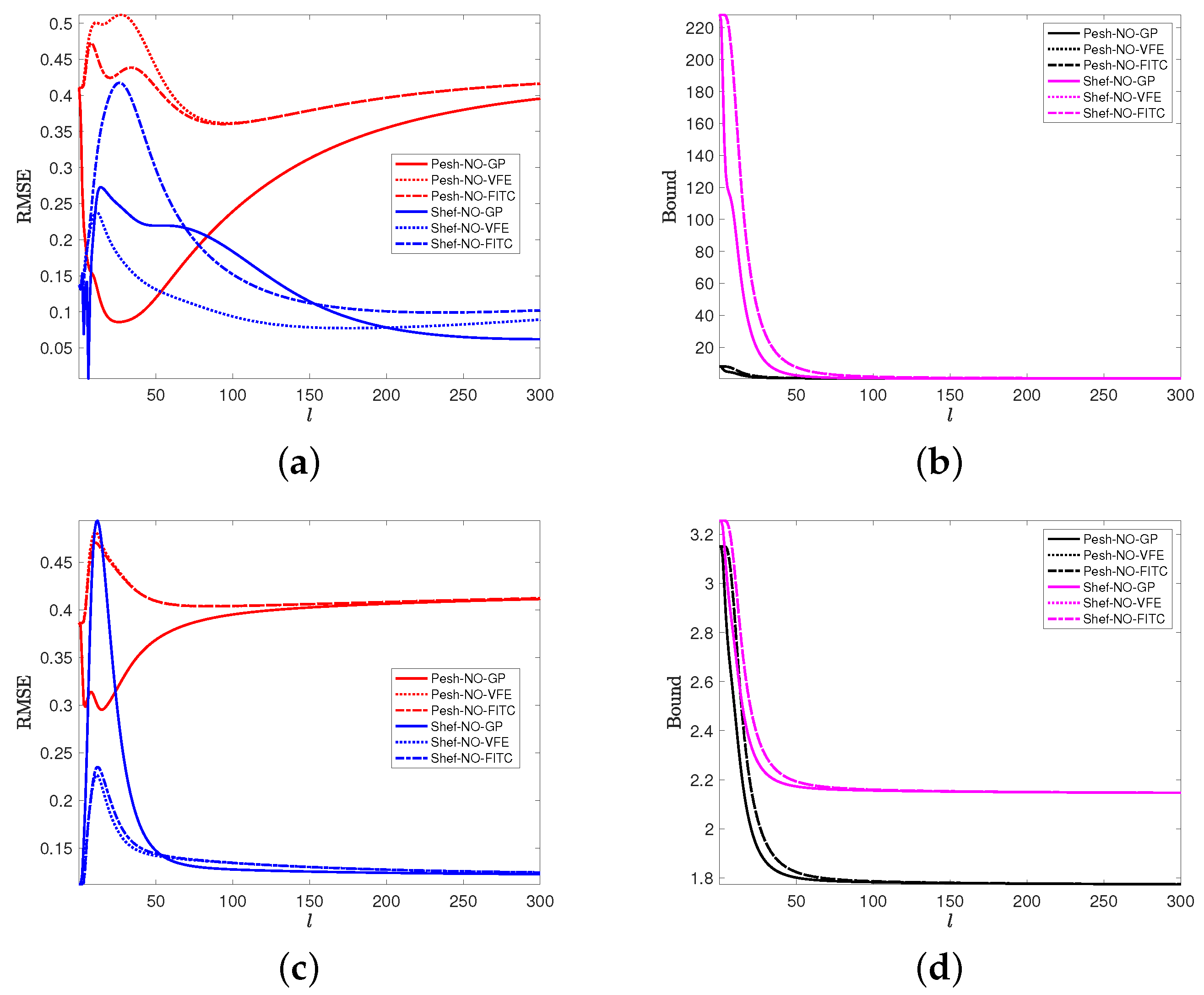
4.3. Impacts of Noise Level on ELBO and UBML
Figure 7 shows the results from Experiment 2. According to our theoretical results, the impact of on the uncertainty should become greater as increases. This is verified by the results shown in Figure 7b,d. Our theoretical results also suggest that the variation of would not affect the prediction accuracy. We can see from Figure 7a,c that when is smaller, it does affect the prediction accuracy, but when it exceeds a certain value, the impacts become negligible. Considering the Neumann series approximation, we would say that the experimental results comply with the theoretical conclusion.
Figure 7.
Relationship of on NO prediction RMSE and uncertainty bound: (a) , (b) , (c) , (d) .
The results of Experiment 3 are shown in Figure 8. We can see that when l is smaller, both RMSE and the uncertainty bounds change rapidly. While after it exceeds certain values, both converge. This again complies with our theoretical conclusions and simulation results. We should also notice from Figure 7 and Figure 8 that the increment of tends to increase the uncertainty, whereas the increment of l tends to decrease the uncertainty. Taking both into consideration, an optimised uncertainty bound can be obtained.
Figure 8.
Relationship of l on NO prediction RMSE and uncertainty bound: (a) , (b) , (c) , (d) .
We also conduct an experiment to demonstrate how the noise level affects the ELBO and UBML. In our experiment, we set to vary from 0.5 to 4.5. The results are shown in Figure 9. To make the results distinguishable, we set the vertical axes to . To make the logrithm work, we reverse the signs of both ELBO and UBML. This is the reason why ELBO is ‘greater’ than UBML in Figure 9. The full GPs model is trained by setting to to obtain 9 sets of hyperparameters. For each set of them, we then set to vary from 0.5 to 4.5. The darker the colour in Figure 9, the smaller is for model training. We can see that generally, greater can slow down the convergence speed of both ELBO and UBML, while training a model. When the model is trained, the increment of can lower down UBML, which is the maximum that ELBO can reach. This implies that the increment of can cause the failure of a sparse GPs model, as ELBO is deeply related to determine a sparse GPs model. Nevertheless, the experimental results again comply with our theoretical conclusions.
Figure 9.
Effects of on ELBO and UBML: (a) NO in Sheffield, (b) NO in Peshawar.
5. Conclusions
This paper proposes a general method to investigate how the performance variation of a Gaussian process model can be attributed to hyperparameters and measurement noises, etc. The method is demonstrated by applying it to process particulate matter (e.g., ) and gaseous pollutants (e.g., NO, , and ) from both Sheffield, UK, and Peshawar, Pakistan. Experimental results show that the proposed method provides insights on how measurement noises and hyperparameters, etc. affect the prediction performance of a Gaussian process. The results align with the analytical derivations, which is enabled by adopting Neuman series to approximate matrix inversions in Gaussian process models. The theoretical findings and experimental results combined demonstrate that the proposed method can generate air quality forecasting results. In the meantime, it provides a way to link uncertainties in measurements and hyperparameters, etc. with the forecasting results. This will help with forecasting performance analysis when measurement noise level or model hyperparameters vary, making the method more general.
Author Contributions
Conceptualization, P.W., L.M., M.M., R.C., S.M., K.A. and M.F.K.; methodology, P.W.; software, P.W.; validation, P.W., Z.Z., C.J. and H.F.; formal analysis, P.W., L.M.; investigation, P.W.; data curation, S.M., R.C., K.A. and M.F.K.; writing—original draft preparation, P.W., L.M., R.C., S.M., K.A. and M.F.K.; writing—review and editing, P.W. and L.M.; visualization, P.W., R.C.; supervision, L.M., M.M.; funding acquisition, L.M., P.W., M.M., S.M. All authors have read and agreed to the published version of the manuscript.
Funding
This research was funded by the UK EPSRC through EP/T013265/1 project NSF-EPSRC:ShiRAS. Towards Safe and Reliable Autonomy in Sensor Driven Systems, a joint project with the USA National Science Foundation under Grant NSF ECCS 1903466. Other funders are NSFC (61703387) and the Global Challenges Research Funds (QR GCRF—Pump priming awards (Round 2), project entitled: “Collaborating with North Pakistan for monitoring and reducing the air pollution (X/160978)”.
Institutional Review Board Statement
Not applicable.
Informed Consent Statement
Not applicable.
Data Availability Statement
Not Applicable.
Acknowledgments
We are grateful to UK EPSRC for funding this work through EP/T013265/1 project NSF-EPSRC:ShiRAS. Towards Safe and Reliable Autonomy in Sensor Driven Systems. This work was also supported by the USA National Science Foundation under Grant NSF ECCS 1903466. We also appreciate the support of NSFC (61703387). We are also grateful to the Global Challenges Research Funds (QR GCRF - Pump priming awards (Round 2), entitled: “Collaborating with North Pakistan for monitoring and reducing the air pollution (X/160978))”. We also thank Urban FLows Observatory, the University of Sheffield for providing the air quality sensors for collecting air pollution data in Pakistan.
Conflicts of Interest
The authors declare no conflict of interest.
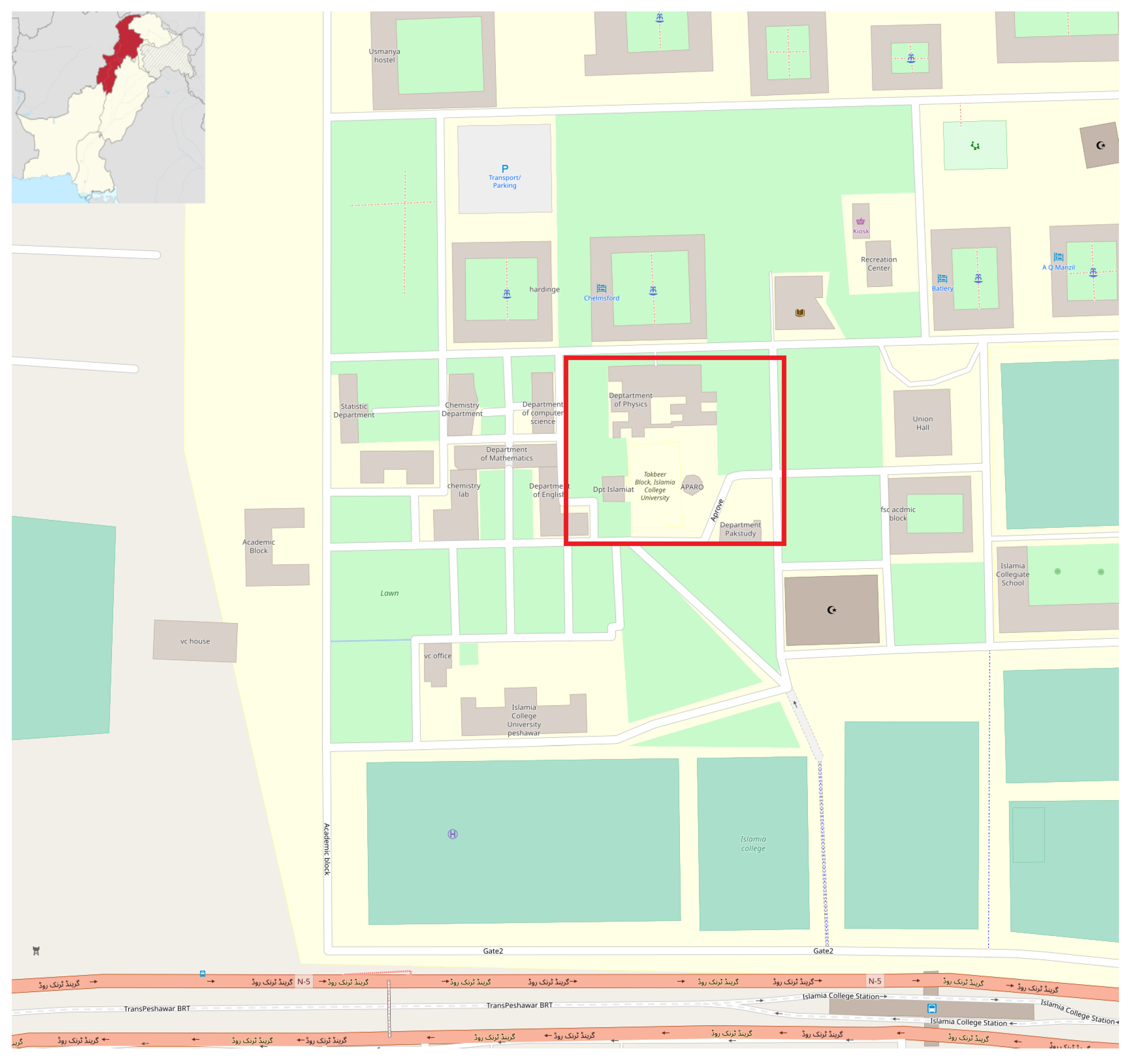
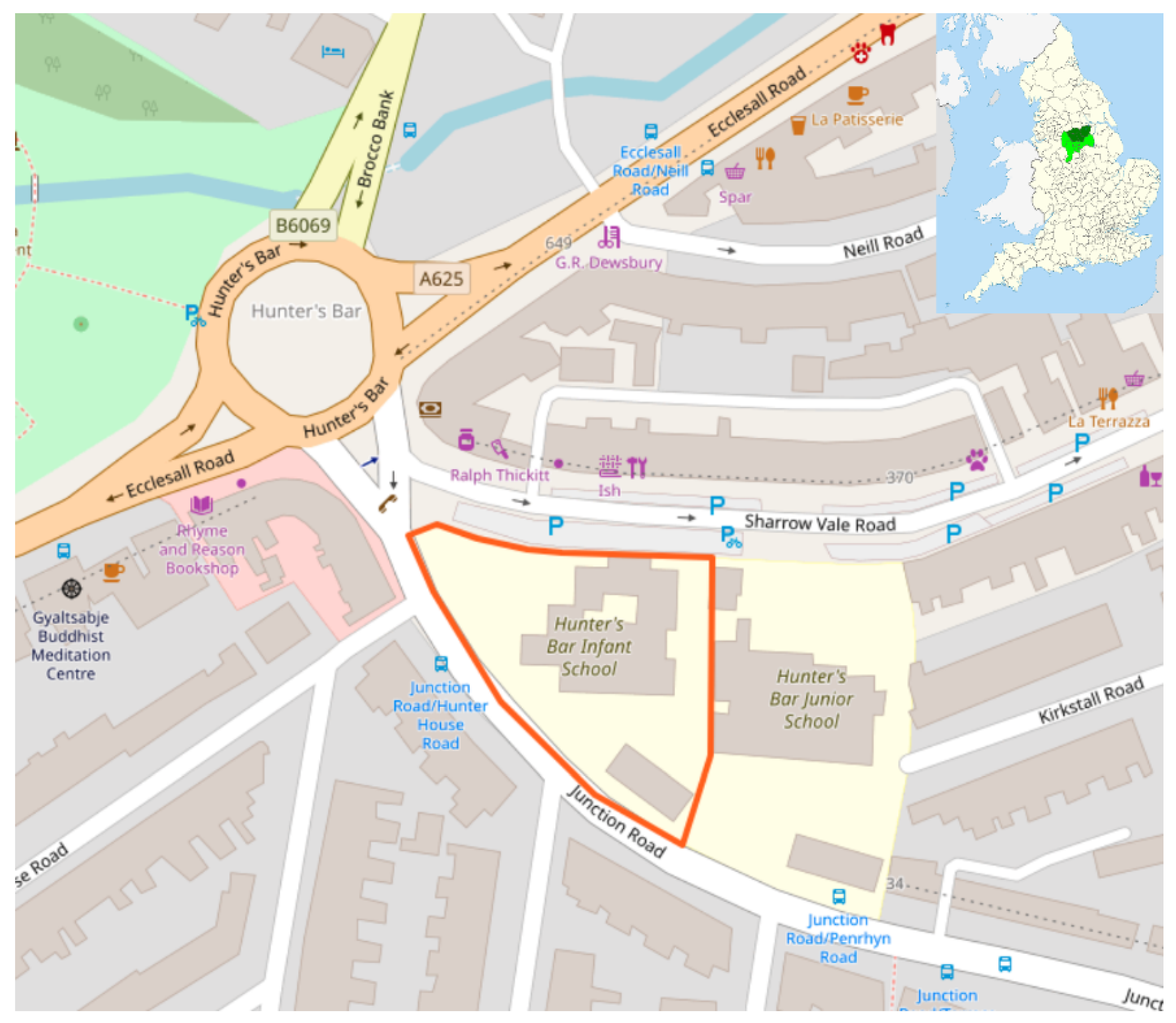
Appendix A. Data Collection
Peshawar (34.015 N, 71.52 E) is a city located in Khyber Pakhtunkhwa, Pakistan, situated at an elevation of 340 m above sea level. Peshawar covers an area of 1257 km and has a population of 1,218,773 making it the biggest city in Khyber Pakhtunkhwa. Peshawar is predominantly hot during summer (May–Mid July) with an average maximum temperature of 40 C followed by monsoon and cold winter.
Local vehicular emission, fossil fuel energy plants and industrial processes are the significant sources of air pollution in Peshawar. Wind direction and wind speed also play a crucial role to observe transboundary pollution build-up. Furthermore, at this site, the distribution and dispersion of air pollution are further impacted by the nearby buildings, and its proximity to Grand Trunk Road, creating a built-up street canyon environment, generated primarily from nearby, increasing traffic pollution.
The air quality monitoring sensor (AQMS) was installed at the University of Peshawar’s Physics Department Building (see Figure A1) at 6 m height from the ground surface level. It is described as an urban background site.
Sheffield ( N, W) is a geographically diverse city located in county South Yorkshire, UK, built on several hills thus situated at an elevation of 29–500 m above sea level. Sheffield covers a total area of 367.9 km with a growing population of 582,506. Sheffield is claimed to be the “greenest city” in England by the local city council. Sheffield enjoys a temperate climate with July considered the hottest month, with an average maximum temperature of 20.8 C.
The air pollution in the city is primarily due to both road transport and industry, and to a lesser extent, fossil fuel-run processes, such as energy supply and commercial or domestic heating systems (for example, wood burners).
The AQMS is installed at 2.5 m height from the elevated ground surface level at the playground of Hunter’s Bar Infants School (see Figure A2), which lies in close proximity to a busy roundabout, and at the intersection of Ecclesall Road, Brocco Bank, Sharrow Vale Road and Junction Road; thus, traffic is the primary source of pollution. It is also described as an urban background site.
Figure A1.
Peshawar study site © OpenStreetMap contributors.
In our case, the AQMSs are commercially low cost sensor nodes AQMesh. They have been deployed at the two sites in Peshawar and Sheffield. A “black box” post calibration is applied to the data by the manufacturer to eliminate the impact of humidity and temperature on the sensor and to eliminate cross sensitivity. The data are aggregated and sampled every 15 min. The data collected from these nodes are transferred to the cloud-based AQMesh database via standard GPRS communication integrated. The data are then accessed through the dedicated API.
Figure A2.
Sheffield study site © OpenStreetMap contributors.
Appendix B. The WHO Concentration Criteria for Pollutants
All data from ’WHO Air quality guidelines for particulate matter, ozone, nitrogen dioxide and sulfur dioxide’ [].
- WHO
Table A1.
WHO Nitrogen dioxide guidelines.
Table A1.
WHO Nitrogen dioxide guidelines.
| Nitrogen Dioxide | Annual Mean | 1-h Mean |
|---|---|---|
- WHO
Table A2.
WHO sulfur dioxide guidelines.
Table A2.
WHO sulfur dioxide guidelines.
| Sulfur Dioxide | 24-h Mean | 10-min Mean |
|---|---|---|
- WHO and
Table A3.
WHO particulate matter guidelines.
Table A3.
WHO particulate matter guidelines.
| Particulate Matter | Annual Mean | 24-h Mean |
|---|---|---|
- WHO
Table A4.
WHO Ozone guidelines.
Table A4.
WHO Ozone guidelines.
| Ozone | 8-h Mean |
|---|---|
Appendix C. Approximated Derivatives of SE Kernel
By specifying a kernel function, we can obtain analytical forms of Equations (28) and (29) immediately. In this paper, we adopt the widely used SE kernel shown in Equation (A1) as an example.
There are two hyperparameters, i.e., the signal variance and length-scale l are involved. Equations (A2) and (A3) show the expectation (prediction mean) partial derivative (EPD) and covariance partial derivative (CPD) of ,
While the derivatives of l are given in Equations (A4) and (A5),
References
- WHO. WHO Global Ambient Air Quality Database (Update 2018); World Health Organization: Geneva, Switzerland, 2018. [Google Scholar]
- Landrigan, P.J. Air pollution and health. Lancet Public Health 2017, 2, e4–e5. [Google Scholar] [CrossRef] [Green Version]
- WHO. Health Effects of Particulate Matter: Policy Implications for Countries in Eastern Europe, Caucasus and Central Asia (2013); World Health Organization Regional Office for Europe: Copenhagen, Denmark, 2013. [Google Scholar]
- Chen, H.; Kwong, J.C.; Copes, R.; Tu, K.; Villeneuve, P.J.; Van Donkelaar, A.; Hystad, P.; Martin, R.V.; Murray, B.J.; Jessiman, B.; et al. Living near major roads and the incidence of dementia, Parkinson’s disease, and multiple sclerosis: A population-based cohort study. Lancet 2017, 389, 718–726. [Google Scholar] [CrossRef]
- Khreis, H.; de Hoogh, K.; Nieuwenhuijsen, M.J. Full-chain health impact assessment of traffic-related air pollution and childhood asthma. Environ. Int. 2018, 114, 365–375. [Google Scholar] [CrossRef] [PubMed]
- Improving Air Quality in the Tackling Nitrogen Dioxide in Our Towns and Cities; UK Overview Document; Department for Environment, Food & Rural Affairs and Department for Transport: London, UK, 2017.
- Rai, A.C.; Kumar, P.; Pilla, F.; Skouloudis, A.N.; Di Sabatino, S.; Ratti, C.; Yasar, A.; Rickerby, D. End-user perspective of low-cost sensors for outdoor air pollution monitoring. Sci. Total Environ. 2017, 607, 691–705. [Google Scholar] [CrossRef] [PubMed] [Green Version]
- Zheng, T.; Bergin, M.H.; Sutaria, R.; Tripathi, S.N.; Caldow, R.; Carlson, D.E. Gaussian process regression model for dynamically calibrating and surveilling a wireless low-cost particulate matter sensor network in Delhi. Atmos. Meas. Tech. 2019, 12, 5161–5181. [Google Scholar] [CrossRef] [Green Version]
- Shen, J. PM2.5 concentration prediction using times series based data mining. City 2012, 2013, 2014–2020. [Google Scholar]
- Silibello, C.; D’Allura, A.; Finardi, S.; Bolignano, A.; Sozzi, R. Application of bias adjustment techniques to improve air quality forecasts. Atmos. Pollut. Res. 2015, 6, 928–938. [Google Scholar] [CrossRef]
- Specht, D.F. A general regression neural network. IEEE Trans. Neural Netw. 1991, 2, 568–576. [Google Scholar] [CrossRef] [PubMed] [Green Version]
- Rumelhart, D.E.; Hinton, G.E.; Williams, R.J. Learning representations by back-propagating errors. Nature 1986, 323, 533–536. [Google Scholar] [CrossRef]
- Lin, K.; Pai, P.; Yang, S. Forecasting concentrations of air pollutants by logarithm support vector regression with immune algorithms. Appl. Math. Comput. 2011, 217, 5318–5327. [Google Scholar] [CrossRef]
- Mao, Y.; Lee, S. Deep Convolutional Neural Network for Air Quality Prediction. J. Phys. Conf. Ser. 2019, 1302, 032046. [Google Scholar] [CrossRef]
- Garriga-Alonso, A.; Rasmussen, C.E.; Aitchison, L. Deep convolutional networks as shallow gaussian processes. arXiv 2018, arXiv:1808.05587. [Google Scholar]
- Bai, L.; Wang, J.; Ma, X.; Lu, H. Air pollution forecasts: An overview. Int. J. Environ. Res. Public Health 2018, 15, 780. [Google Scholar] [CrossRef] [PubMed] [Green Version]
- Wang, P.; Mihaylova, L.; Munir, S.; Chakraborty, R.; Wang, J.; Mayfield, M.; Alam, K.; Khokhar, M.F.; Coca, D. A computationally efficient symmetric diagonally dominant matrix projection-based Gaussian process approach. Signal Process. 2021, 183, 108034. [Google Scholar] [CrossRef]
- Burt, D.R.; Rasmussen, C.E.; Van Der Wilk, M. Rates of Convergence for Sparse Variational Gaussian Process Regression. arXiv 2019, arXiv:1903.03571. [Google Scholar]
- Liu, H.; Ong, Y.S.; Shen, X.; Cai, J. When Gaussian process meets big data: A review of scalable GPs. IEEE Trans. Neural Netw. Learn. Syst. 2020, 31, 4405–4423. [Google Scholar] [CrossRef] [PubMed] [Green Version]
- Williams, C.K.; Rasmussen, C.E. Gaussian Processes for Machine Learning; Number 3; MIT Press: Cambridge, MA, USA, 2006. [Google Scholar]
- Wu, M.; Yin, B.; Wang, G.; Dick, C.; Cavallaro, J.R.; Studer, C. Large-scale MIMO detection for 3GPP LTE: Algorithms and FPGA implementations. IEEE J. Sel. Top. Signal Process. 2014, 8, 916–929. [Google Scholar] [CrossRef] [Green Version]
- Chen, Z.; Wang, B. How priors of initial hyperparameters affect Gaussian process regression models. Neurocomputing 2018, 275, 1702–1710. [Google Scholar] [CrossRef] [Green Version]
- Zhu, D.; Li, B.; Liang, P. On the matrix inversion approximation based on Neumann series in massive MIMO systems. In Proceedings of the 2015 IEEE International Conference on Communications (ICC), London, UK, 8–12 June 2015; pp. 1763–1769. [Google Scholar]
- Titsias, M. Variational learning of inducing variables in sparse Gaussian processes. In Proceedings of the Artificial Intelligence and Statistics, Clearwater Beach, FL, USA, 16–18 April 2009; pp. 567–574. [Google Scholar]
- Snelson, E.; Ghahramani, Z. Sparse Gaussian processes using pseudo-inputs. In Proceedings of the Advances in Neural Information Processing Systems, Vancouver, Canada, 4–9 December 2006; pp. 1257–1264. [Google Scholar]
- WHO. Air Quality Guidelines for Particulate Matter, Ozone, Nitrogen Dioxide and Sulphur Dioxide. Global Update 2005; World Health Organization: Geneva, Switzerland, 2006. [Google Scholar]
Publisher’s Note: MDPI stays neutral with regard to jurisdictional claims in published maps and institutional affiliations. |
© 2021 by the authors. Licensee MDPI, Basel, Switzerland. This article is an open access article distributed under the terms and conditions of the Creative Commons Attribution (CC BY) license (https://creativecommons.org/licenses/by/4.0/).