Abstract
Tropospheric ozone (O3) levels in southern Europe have an increasing tendency, in close relation with the higher incidence of hot summers and heatwaves. Given that O3 is one of the most damaging pollutants for vegetation, known to affect productivity and quality of crops, it is necessary to develop more rigorous and consistent methods of risk assessment that consider climate change conditions. Studying the O3 deposition over the Douro Demarcated Region (DDR), which is one of the most productive wine areas in Portugal, and assessing its potential effects under a climate change scenario, was the purpose of this study. To that end, the chemical transport model CHIMERE, with a spatial resolution of 1 km2, fed by meteorological data from the WRF model, was applied for a recent past climate (2003 to 2005) and future mid-term (2049 and 2064) and long-term (2096 and 2097) scenarios. Simulations for future climate were performed considering: (i) only the climate change effect, and (ii) the effect of climate change together with future air pollutant emissions. The assessment of the potential damage in terms of wine productivity and quality (sugar content) was performed through analysis of O3 deposition and the application of concentration–response functions, based on AOT40 values. Modeling results show that a reduction in emission of O3 precursors can successfully decrease AOT40 levels in the DDR, but it is not enough to accomplish the European Commission target value for the protection of vegetation. If the emissions remain constant, the exposure–response functions indicate that, in the long-term, AOT40 levels could worsen wine productivity and quality.
1. Introduction
Air pollution and climate change are closely related. Air pollutants and their precursors are often co-emitted with carbon dioxide (CO2) or other Green House Gases, and air pollutant emissions can cause warming or cooling effects on the climate. In turn, climate change influences air pollution by altering the frequency, severity, and duration of heatwaves, air-stagnation events, precipitation, and other weather changes that result in pollutant accumulation [1,2,3,4,5,6]. Identifying the co-benefits of reducing air pollutants that also reduce the impacts of climate change is an important contribution to climate change research and mitigation.
Tropospheric ozone (O3) levels in southern Europe have an increasing tendency, which is related to the higher incidence of hot summers and heatwaves [1,7,8,9]. Modeling results indicate that climate change alone will cause O3 concentrations to increase in many regions in the world [10,11,12]. For instance, under the RCP8.5 scenario, Lacressonnière et al. [10] estimated an increase in O3 levels of approximately 1.5 ppb per decade, during the summer in Europe. Similarly, Sá et al. [11] estimated an increase in the occurrence, duration, and intensity of extreme O3 values in Northern Portugal. In addition to weather conditions, such as temperature, humidity, cloud cover, and winds, O3 concentrations depend on emissions of its precursors as well as long-range transport [13].
Working towards a reduction in O3 concentrations is very important due to the effects of O3 on human health and vegetation. However, due to the complex and non-linear chemistry of O3, reducing the emissions from its precursors may not lead to a decrease in its concentrations. A specific study for Portugal [14] showed that, despite the reduction in O3 precursors’ emissions imposed by the National Emission Ceilings Directive, mean tropospheric ozone concentrations significantly increased between 2003 and 2007 although the number of exceedances to the information threshold (180 μg·m−3) decreased. O3 is the most damaging air pollutant to crop yield quantity and quality [15,16,17,18]. Avnery et al. [19,20] estimated that, globally, surface O3 reduced the yields of key crops by up to 15% in 2000 and is projected to cause a 26% reduction in 2030. Blanco-Ward et al. [17], in their review of tropospheric O3 phytotoxic effects on the grapevine, mention potential yield reductions in the range of 20–31%, as well as damages of grape quality, due to reductions in total polyphenols, in the range of 15–23%. Ascenso et al. [21] estimated that the Douro Demarcated Region (DDR) vineyards’ current exposure to O3 could result in a productivity loss of up to 27%.
Due to its economic interest, the impacts of climate change on wine production have been studied by many authors (e.g., [22,23,24,25,26]), but few address the complex relationship between surface O3 concentrations, climate change, and grapevine productivity and quality [27]. The DDR is an important wine region in Portugal, where the famous Port Wine is produced. Located within the Douro River basin in the northeastern part of Portugal, the region is known for its deep valleys and mountainous terrain. The main objective of this study was to evaluate Douro vineyards’ exposure to tropospheric O3 in future climates, by assessing O3 concentrations and deposition in the DDR and then evaluating the potential damage in terms of productivity and quality (sugar loss).
2. Methodology
O3 concentration and dry deposition were estimated using the air-quality modeling system WRF-CHIMERE. The simulations were performed for the hottest years of the recent past and mid- and long-term future conditions. The AOT40 (accumulated concentration of O3 above 40 ppb) indicator, proposed by the European Union to monitor and prevent vegetation damage from O3 exposure, was calculated and used as input data to estimate the potential loss of productivity and grape sugar content due to climate change, and also considering the projected O3 precursors’ emissions.
2.1. WRF-CHIMERE Modeling System
Climate numerical simulations were performed using the regional high-resolution Weather Research and Forecasting v3.5.1 (WRF) model with two distinct forcings (initial conditions and boundary conditions), namely, ERA-Interim reanalysis [28] and the Max Planck Institute Earth System Model—low resolution (MPI-ESM-LR) [29]. The MPI-ESM-LR model was developed by the MPI with a horizontal resolution of 1.9° [30]. This model participated in the Coupled Model Intercomparison Project Phase 5 (CMIP5) that considered future greenhouse gas emission scenarios defined by the Representative Concentration Pathways (RCP) [31]. In particular, this study considered the RCP8.5 scenario (Radiative Forcing: >8.5 W/m2 in 2100; Concentration: >~1370 CO2-eq in 2100; Pathway shape: Rising) [32].
The CHIMERE model (v2016a1) was used in this study. CHIMERE is an open access multi-scale Eulerian chemical transport model (CTM) that applies the integration of the mass continuity equation to estimate the concentrations of several chemical species in each cell of a given grid. It was developed for simulating gas-phase chemistry [33], aerosol formation, transport, and deposition [34] from regional to urban scales. As input data, the CHIMERE model requires meteorology (from WRF), initial and boundary conditions (from MOZART; [35]), atmospheric emissions (from EMEP; [36]), and land use and topography data (from USGS). For more details on the model parametrizations and input data, see Ascenso et al. [21].
The air-quality simulations for the future climate were two-fold: one was performed considering climate change only, i.e., emissions were kept the same as in recent past climate simulations, to assess the contribution to O3 levels of meteorological variables alone; the other also included future projected emissions to assess future O3 levels resulting from both contributions (meteorology and emissions).
The application of the air-quality modeling system WRF-CHIMERE was set up in a one-way hourly nesting configuration with four nested domains with an increasing horizontal resolution. The last domain was focused on the DDR, with a spatial resolution of 1 km2. For a detailed description of the DDR case study, see Ascenso et al. [21]. The simulation periods were selected based on a climatologic assessment of the region that identified the hottest years from an historical period (1986–2005) and mid- (2046–2065) and long-term (2081–2100) projected scenarios, which were based on the RCP8.5 pathway. The 20-year periods considered for this assessment were the same as those considered in the 5th Intergovernmental Panel on Climate Change (IPCC) Assessment Report [37]. The years 2003 to 2005 were chosen to simulate the recent past climate, 2049 and 2064 for the mid-term future climate, and the years 2096 and 2097 for the long-term future climate.
In addition to meteorological data, emissions are one of the main input data for air-quality modeling, both for the recent past and for the future climate scenarios. For the recent past scenario, 2005 emissions from the EMEP database [36] were used. For future emissions, a methodology to project anthropogenic emissions from the EMEP database was developed. The estimation of future emissions was founded on the RCP8.5 emission scenario [38], keeping therefore consistency between the climate change simulations and the air-quality simulations. This methodology was based on Equation (1):
The EMEP emission inventory for the year 2005 was, therefore, selected to project emissions to the mid- and long-term future scenarios, using RCP8.5 scenario emission data with the same spatial resolution of the EMEP grid (0.5 degrees by grid cell) as a normalization factor to those future projections. A few adjustments between the EMEP and the RCP approaches were performed, namely, correspondence by activity sectors, adopting the Selected Nomenclature for Air Pollution (SNAP): 1—Public power stations, 2—Residential combustion plants, 3—Industrial combustion, 4—Production processes, 5—Extraction and distribution of fossil fuels, 6—Solvent use, 7—Road transport, 8—Other mobile sources. Figure 1 shows the relative differences between 2005 inventory emissions and 2050 and 2100 projected emissions for the O3 precursors nitrogen dioxide (NO2) and non-methane volatile organic compounds (NMVOC).
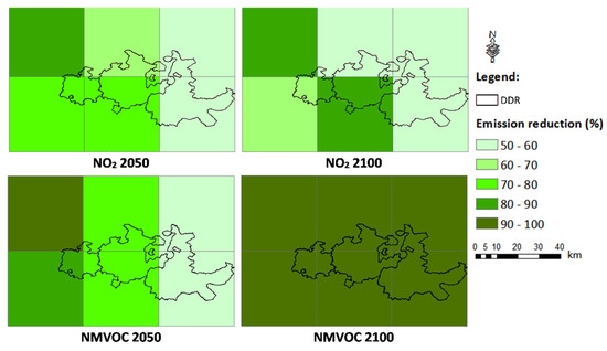
Figure 1.
Spatial distribution of NO2 and NMVOC emissions reduction (%) for the DDR EMEP cells in 2050 and 2100.
The emission projections for NO2 and NMVOC indicated a marked reduction in both pollutants (>50%). The main driver for NO2 emissions reduction was the road transport sector (SNAP 7). In contrast, NO2 emissions from other mobile sources and machinery (SNAP8) were expected to increase in the future, mainly due to a rise in air and sea traffic [39,40].
Regarding NMVOC, the main emission sectors were solvent and other product use (SNAP6) and road transport (SNAP 7); according to the RCP8.5 future projections, emissions of these chemical compounds will be widely reduced.
In summary, a set of five scenarios and a total of 11 yearly simulations were analyzed (Table 1).

Table 1.
Summary of the methodology for each scenario assessed in this study. Legend: BASE—Simulation of the recent past climate; MT—Mid-term simulation; MT_emis—Mid-term simulation with projected emissions; LT—Long-term simulation; LT_emis—Long-term simulation with projected emissions.
2.2. Vineyards’ Exposure to Ozone
To evaluate the risk of Douro vineyards’ exposure to O3, the accumulated exposure indicator AOT40 was calculated and averaged for the simulated years in each scenario. According to the Directive 2008/50/EC of the European Parliament and of the Council of 21 May 2008 on ambient air quality and cleaner air for Europe (see Annex VII, point A1), “AOT40 (expressed in (μg·m−3)∙hours) means the sum of the difference between hourly concentrations greater than 80 μg·m−3 (= 40 parts per billion) and 80 μg·m−3 over a given period using only the one-hour values measured between 8.00 and 20.00 Central European Time (CET) each day”. Note that 80 μg·m−3 of ozone is approximately 40 ppb because the unit conversion depends on the density of the air. The European and Portuguese target value is 18,000 μg·m−3·h averaged over five years. The long-term objective is 6000 μg·m−3·h. AOT40 quantifies only O3 exposure, i.e., not the effective O3 uptake by (and therefore damage caused to) vegetation. Thus, O3 deposition simulated levels are also presented and discussed.
The assessment of the potential damage in terms of productivity and quality was performed through the application of the exposure–response functions calculated by Soja et al. [41] in their three-year experimental study on the effects of long-term ozone exposure in pot-grown grapevines, regarding fruit yield, noted in Equation (2), and sugar concentrations in juice, noted in Equation (3), wherein grapevines were exposed to different ozone levels in open-top chambers.
In these Soja et al. [41] equations, AOT40 is expressed in µmol·mol−1·h. For this work, the function applied was the one calculated for the last year of the experiment, meaning that this exposure–response function assumed that grapevines were exposed to constant levels of ozone for three years.
3. Effects of Ozone on Vineyards
The effects of O3 on the vineyards were based on the AOT40 indicator, productivity and quality losses, and dry deposition estimated values, for the different simulated scenarios.
3.1. AOT40
Figure 2 shows the BASE scenario AOT40 simulated values based on the modeling results averaged over the three recent past simulation years (2003–2004–2005).
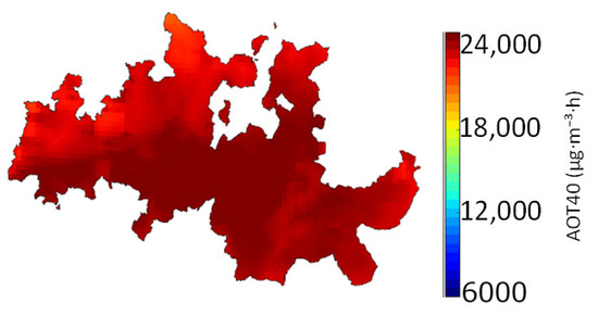
Figure 2.
AOT40 levels (μg·m−3·h) in the DDR for the BASE scenario, averaged over the three recent past years (1 × 1 km2 horizontal resolution).
Exceedances of the target value for vegetation protection (18,000 μg·m−3·h) occurred throughout the DDR area for the recent past conditions. The average AOT40 level for the recent past was 22,500 μg·m−3·h. This area of Portugal is known for its high O3 values, observed at the Douro Norte air-quality monitoring station and estimated through modeling approaches [42,43,44]. The average O3 concentration in the Douro Norte monitoring station for 2003–2005 was 106 µg∙m−3 with an hourly maximum of 361 µg∙m−3. The high values were related to high altitudes, long-range transport (eastern synoptic forcing), and sea-breeze circulation [45,46].
The maximum level, calculated (24,000 μg·m−3·h) in the central area of the DDR, was about 1.3 times higher than the target value. This zone also has the lowest wine production per unit of area in the DDR [47].
Figure 3 shows the AOT40 results for the climate change scenarios, with and without emission projected changes.
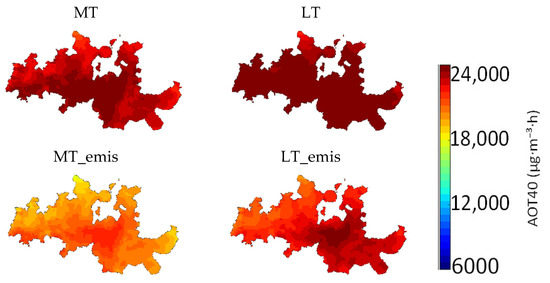
Figure 3.
AOT40 values (μg·m−3·h) for mid-term and long-term climate change scenarios in the DDR (1 × 1 km2 horizontal resolution). Legend: MT—Mid-term simulation; MT_emis—Mid-term simulation with projected emissions; LT—Long-term simulation; LT_emis—Long-term simulation with projected emissions.
For the MT scenario, no relevant differences were estimated in relation to the BASE scenario, with an average reduction of 1% in AOT40 levels, due to the small changes in meteorological conditions. On the other hand, AOT40 levels decreased by 20% in the MT_emis scenario, indicating that the reduction in AOT40 levels was mainly influenced by the reduction in emissions.
The greatest differences in AOT40 levels were estimated to occur in the long-term future. In the LT scenario, the model results showed that the impact of climate change on the O3 concentration would result in a 7% increase in AOT40 levels (Figure 3). Although AOT40 levels would continue to exceed the target value for vegetation protection, when projected emissions were considered (LT_emis scenario), AOT40 levels would decrease by an average of 8% in relation to the BASE scenario.
3.2. Productivity and Quality Losses
Figure 4 shows the BASE values for grapevine productivity and quality loss due to O3 exposure. The impact on quality was calculated through the changes in the grape’s sugar content, an important indicator for wine quality.

Figure 4.
Productivity change (%) (left) and quality change (%) (right), for the BASE scenario, based on Soja et al. [41] exposure–response functions.
In the BASE scenario, the exposure to high AOT40 levels led to an average productivity loss of 27% and a quality loss of 32%, following Soja et al. [41] response functions. The spatial distribution was similar to that in the AOT40 maps since this indicator was the only variable in the exposure–response functions. These results show that the quality indicator was more sensitive to O3 exposure when compared to productivity; O3 decreased the photosynthetic capacity of leaves and shifted the partitioning of available carbohydrates [41].
The climate change and emission reduction impact on productivity and quality loss for the mid-term and long-term future is presented in Figure 5 and Figure 6, respectively.
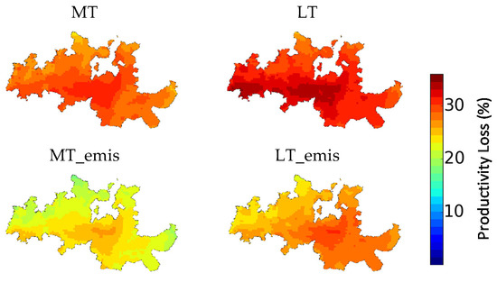
Figure 5.
Productivity Loss (%) for mid-term and long-term climate change scenarios in the DDR (1 × 1 km2 horizontal resolution). Legend: MT—Mid-term simulation; MT_emis—Mid-term simulation with projected emissions; LT—Long-term simulation; LT_emis—Long-term simulation with projected emissions.
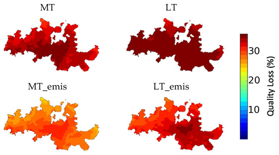
Figure 6.
Quality loss (%) for mid-term and long-term climate change scenarios in the DDR (1 × 1 km2 horizontal resolution). Legend: MT—Mid-term simulation; MT_emis—Mid-term simulation with projected emissions; LT—Long-term simulation; LT_emis—Long-term simulation with projected emissions.
Akin to the previous discussed AOT40 levels, relative differences between future scenarios and the BASE case showed an average reduction of 1% in productivity and quality for the MT scenario. For the MT_emis scenario, the 20% decrease in AOT40 levels would lead to a reduction of 5% in productivity losses and 6% in sugar content (grape quality). In the LT scenario, the model results show that the impact of climate change on the O3 concentration would result in a 9% and 7% increase in productivity and quality losses, respectively. However, if the projected emissions reduction were to happen, a decrease of 8% in productivity losses and 7% in quality losses would be expected, relatively to the BASE scenario.
When discussing these outcomes, it is important to take into account that extrapolating Soja et al. [41] functions to the Douro vineyards has some limitations. The functions were based on a reduced number of replicated experiments with only one cultivar (which is different from DDR’s cultivars), and maximum stomatal conductances can differ with age and variety for the grapevine, and can also differ between control studies and the field. Moreover, inferring empirical information obtained under current climatic conditions to assess future risks also brings uncertainty as quality and productivity also change in response to climate change and technological development.
Balancing these results with the reported wine production over the years in the DDR (Figure 7), a reduction in the production of wine is visible a couple of years after the study period (hot years compared to the climatological normal of the recent past). This indicates that environmental stresses can cumulatively affect vineyards. However, it is not possible to compare such values with the study results, since many factors can influence wine production and, in this study, the effect of O3 exposure was assessed isolated from other variables. While O3 could have been reducing productivity, other factors such as temperature, precipitation, and humidity could improve it.
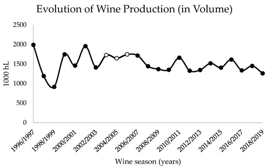
Figure 7.
Evolution of wine production in the Douro wine region from 1996 to 2018, according to Instituto da Vinha e do Vinho, I.P annual reports [48]. The study period (2004 to 2005) is highlighted in white.
3.3. Ozone Dry Deposition
The deposition level results were based on the total O3 dry deposition accumulated over May to July, the same period established in the Air Quality Framework Directive 2008/50/CE for the calculation of the AOT40 indicator [21]. Figure 8 shows the BASE scenario O3 dry deposition values, and in Figure 9 the results for the future climate scenarios are presented.
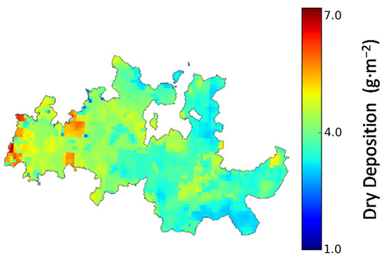
Figure 8.
BASE O3 dry deposition (g·m−2) in DDR (1 × 1 km2 horizontal resolution), accumulated from May to July and averaged for the three simulation years.
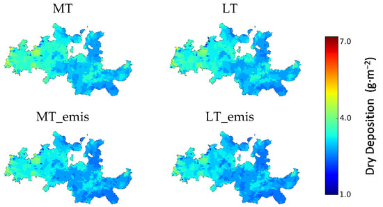
Figure 9.
O3 dry deposition (g·m−2) results for mid-term and long-term future climates. Legend: MT—Mid-term simulation; MT_emis—Mid-term simulation with projected emissions; LT—Long-term simulation; LT_emis—Long-term simulation with projected emissions.
The average BASE value of O3 dry deposition was approximately 4 g·m−2 (deposition velocity ~0.64 cm/s). Higher values were observed over the west side of the DDR, due to the higher precipitation and lower temperatures observed in this area. The spatial distribution of AOT40 and deposition values were distinct, suggesting that exposure-based indicators were not the best approach to assess O3 damage to vegetation [21].
The dry deposition values of O3 for the MT and MT_emis scenarios were similar, decreasing 33% and 37% in relation to the BASE scenario. The same was seen for LT and LT_emis scenario results, where decreases of 30% and 34%, respectively, are estimated. These results indicate that, unlike AOT40 levels, dry deposition was mostly influenced by meteorological factors. Therefore, even with an increase in O3 concentrations, the risk of damage to vegetation is expected to decrease. Analogous conclusions were drawn by Klingberg et al. [49].
The projected reduction in O3 dry deposition was mostly related to increasing stress factors on the stomata, such as drier conditions and higher temperatures. The modeling results show that, for both future scenarios, an increase in temperature is expected in the DDR, in particular for maximum temperatures during the summer season. This warming trend will lead to a substantial increase in tropical nights. Moreover, for the long-term climate, it is predicted that the majority of the summer season will be under heatwave conditions. A decrease in precipitation is also expected, leading to a large increase in the number of consecutive dry days and a decrease in consecutive wet days, particularly for the long-term climate.
4. Summary and Conclusions
The complex interactions of natural variability and changes in climate and emissions pose a significant challenge for air-quality management. Some approaches to mitigate climate change could result in large near-term co-benefits for air quality. Moreover, given the effects of ambient O3 on crops and natural vegetation, it becomes necessary to develop more reliable methods of risk assessment that consider the specific environmental conditions of these areas.
This work aimed to estimate O3 concentration and deposition over the DDR for the recent past, mid- and long-term future, to assess the potential effects of Douro vineyards’ exposure to O3. Simulations for the future climate were performed only considering the climate change impact in O3 concentrations and considering projected emissions as well. Table 2 summarizes the O3 effects on Douro vineyards for the mid-term and long-term future, based on RCP8.5 climate projection.

Table 2.
Summary of O3 effects on Douro vineyards for mid-term and long-term climate, based on RCP8.5 climate projection. Legend: BASE—Simulation for the current climate; MT—Mid-term simulation; MT_emis—Mid-term simulation with projected emissions; LT—Long-term simulation; LT_emis—Long-term simulation with projected emissions.
Modeling results show that a reduction in emission of O3 precursors can successfully decrease the AOT40 levels in the Douro Region. Nonetheless, the emission reduction projected by RCP8.5 would not be enough to accomplish the target value for the protection of vegetation established in the Air Quality Framework Directive since this value is exceeded over the entire region, suggesting a likely negative impact for crops. If the projected emissions are considered, the exposure–response functions indicate that, in the long-term, AOT40 levels can represent potential damage to the grapevines causing over 30% loss in quality, which is less than the estimated impact in the recent past scenario.
The O3 dry deposition levels also suggest a decrease in the potential damage to the DDR’s vineyards, however, these results were observed for all scenarios, unlike the AOT40 indicator. Thus, the O3 effects on Douro vineyards based on the AOT40 may be overestimated. It is important to define a threshold for the protection of vegetation that considers the potential uptake using dry deposition levels and developing crop-specific dose–response functions.
Author Contributions
Conceptualization, A.A., M.L. and A.I.M.; formal analysis, A.A.; investigation, A.A., C.G., C.S. and C.V.; project administration, C.S. and A.I.M.; software, A.A., C.G. and C.V.; supervision, A.R. and A.I.M.; visualization, A.A.; writing—original draft, A.A.; writing—review and editing, A.A., C.G., C.S., C.V., A.R., M.L. and A.I.M. All authors have read and agreed to the published version of the manuscript.
Funding
The authors wish to thank the financial support of FEDER through the COMPETE Program and the national funds from FCT—Science and Technology Portuguese Foundation for financing the DOUROZONE project (PTDC/AAG-MAA/3335/2014; POCI-01-0145-FEDER-016778). Thanks is also due for the financial support to the PhD grant of A. Ascenso (SFRH/BD/136875/2018). Thanks is due to FCT/MCTES for the financial support to CESAM (UIDP/50017/2020+UIDB/50017/2020), through national funds.
Institutional Review Board Statement
Not applicable.
Informed Consent Statement
Not applicable.
Data Availability Statement
Data set available on request to corresponding authors.
Conflicts of Interest
The authors declare no conflict of interest.
References
- Jacob, D.J.; Winner, D.A. Effect of climate change on air quality. Atmos. Environ. 2009, 43, 51–63. [Google Scholar] [CrossRef]
- Fiore, A.M.; Naik, V.; Leibensperger, E.M. Air Quality and Climate Connections. J. Air Waste Manag. Assoc. 2015, 65, 645–685. [Google Scholar] [CrossRef] [PubMed]
- Fiore, A.M.; Naik, V.; Spracklen, D.V.; Steiner, A.; Unger, N.; Prather, M.; Bergmann, D.; Cameron-Smith, P.J.; Cionni, I.; Collins, W.J.; et al. Global air quality and climate. Chem. Soc. Rev. 2012, 41, 6663–6683. [Google Scholar] [CrossRef]
- Reid, N.; Misra, P.K.; Amman, M.; Hales, J. Air Quality Modeling for Policy Development. J. Toxicol. Environ. Health Part A 2007, 70, 295–310. [Google Scholar] [CrossRef]
- Camalier, L.; Cox, W.; Dolwick, P. The effects of meteorology on ozone in urban areas and their use in assessing ozone trends. Atmos. Environ. 2007, 41, 7127–7137. [Google Scholar] [CrossRef]
- Carvalho, A.; Monteiro, A.; Solman, S.; Miranda, A.I.; Borrego, C. Climate-driven changes in air quality over Europe by the end of the 21st century, with special reference to Portugal. Environ. Sci. Policy 2010, 13, 445–458. [Google Scholar] [CrossRef]
- Katragkou, E.; Zanis, P.; Kioutsioukis, I.; Tegoulias, I.; Melas, D.; Krger, B.C.; Coppola, E. Future climate change impacts on summer surface ozone from regional climate-air quality simulations over Europe. J. Geophys. Res. Atmos. 2011, 116, 1–14. [Google Scholar] [CrossRef]
- Meleux, F.; Solmon, F.; Giorgi, F. Increase in summer European ozone amounts due to climate change. Atmos. Environ. 2007, 41, 7577–7587. [Google Scholar] [CrossRef]
- Sitch, S.; Cox, P.M.; Collins, W.J.; Huntingford, C. Indirect radiative forcing of climate change through ozone effects on the land-carbon sink. Nature 2007, 448, 791–794. [Google Scholar] [CrossRef] [PubMed]
- Lacressonnière, G.; Peuch, V.-H.; Vautard, R.; Arteta, J.; Déqué, M.; Joly, M.; Josse, B.; Marécal, V.; Saint-Martin, D. European air quality in the 2030s and 2050s: Impacts of global and regional emission trends and of climate change. Atmos. Environ. 2014, 92, 348–358. [Google Scholar] [CrossRef]
- Sá, E.; Martins, H.; Ferreira, J.; Marta-Almeida, M.; Rocha, A.; Carvalho, A.; Freitas, S.; Borrego, C. Climate change and pollutant emissions impacts on air quality in 2050 over Portugal. Atmos. Environ. 2016, 131, 209–224. [Google Scholar] [CrossRef]
- Andersson, C.; Engardt, M. European ozone in a future climate: Importance of changes in dry deposition and isoprene emissions. J. Geophys. Res. Atmos. 2010, 115, 2303. [Google Scholar] [CrossRef]
- Lu, X.; Zhang, L.; Shen, L. Meteorology and Climate Influences on Tropospheric Ozone: A Review of Natural Sources, Chemistry, and Transport Patterns. Curr. Pollut. Rep. 2019, 5, 238–260. [Google Scholar] [CrossRef]
- Barros, N.; Fontes, T.; Silva, M.P.; Manso, M.C.; Carvalho, A.C. Analysis of the effectiveness of the NEC Directive on the tropospheric ozone levels in Portugal. Atmos. Environ. 2015, 106, 80–91. [Google Scholar] [CrossRef]
- Mills, G.; Hayes, F.; Simpson, D.; Emberson, L.; Norris, D.; Harmens, H.; Büker, P. Evidence of widespread effects of ozone on crops and (semi-)natural vegetation in Europe (1990–2006) in relation to AOT40- and flux-based risk maps. Glob. Chang. Biol. 2011, 17, 592–613. [Google Scholar] [CrossRef]
- Booker, F.; Muntifering, R.; Mcgrath, M.; Burkey, K.; Decoteau, D.; Fiscus, E.; Manning, W.; Krupa, S.; Chappelka, A.; Grantz, D. The ozone component of global change: Potential effects on agricultural and horticultural plant yield, product quality and interactions with invasive species. J. Integr. Plant Biol. 2009, 51, 337–351. [Google Scholar] [CrossRef] [PubMed]
- Blanco-Ward, D.; Rocha, A.; Viceto, C.; Ribeiro, A.C.; Feliciano, M.; Paoletti, E.; Miranda, A.I. Validation of meteorological and ground-level ozone WRF-CHIMERE simulations in a mountainous grapevine growing area for phytotoxic risk assessment. Atmos. Environ. 2021, 259, 118507. [Google Scholar] [CrossRef]
- Juráň, S.; Grace, J.; Urban, O. Temporal Changes in Ozone Concentrations and Their Impact on Vegetation. Atmosphere 2021, 12, 82. [Google Scholar] [CrossRef]
- Avnery, S.; Mauzerall, D.L.; Liu, J.; Horowitz, L.W. Global crop yield reductions due to surface ozone exposure: 1. Year 2000 crop production losses and economic damage. Atmos. Environ. 2011, 45, 2284–2296. [Google Scholar] [CrossRef]
- Avnery, S.; Mauzerall, D.L.; Liu, J.; Horowitz, L.W. Global crop yield reductions due to surface ozone exposure: 2. Year 2030 potential crop production losses and economic damage under two scenarios of O3 pollution. Atmos. Environ. 2011, 45, 2297–2309. [Google Scholar] [CrossRef]
- Ascenso, A.; Gama, C.; Blanco-Ward, D.; Monteiro, A.; Silveira, C.; Viceto, C.; Rodrigues, V.; Rocha, A.; Borrego, C.; Lopes, M.; et al. Assessing Douro Vineyards Exposure to Tropospheric Ozone. Atmosphere 2021, 12, 200. [Google Scholar] [CrossRef]
- Blanco-Ward, D.; Monteiro, A.; Lopes, M.; Borrego, C.; Silveira, C.; Viceto, C.; Rocha, A.; Ribeiro, A.; Andrade, J.; Feliciano, M.; et al. Climate change impact on a wine-producing region using a dynamical downscaling approach: Climate parameters, bioclimatic indices and extreme indices. Int. J. Climatol. 2019, 39, 5741–5760. [Google Scholar] [CrossRef]
- Martins, J.; Fraga, H.; Fonseca, A.; Santos, J.A. Climate Projections for Precipitation and Temperature Indicators in the Douro Wine Region: The Importance of Bias Correction. Agrony 2021, 11, 990. [Google Scholar] [CrossRef]
- Fraga, H.; Santos, J.A.; Malheiro, A.C.; Moutinho-Pereira, J. Climate change projections for the portuguese viticulture using a multi-model ensemble. Cienc. Tec. Vitivinic. 2012, 27, 39–48. [Google Scholar]
- van Leeuwen, C.; Schultz, H.R.; Garcia de Cortazar-Atauri, I.; Duchêne, E.; Ollat, N.; Pieri, P.; Bois, B.; Goutouly, J.-P.; Quénol, H.; Touzard, J.-M.; et al. Why climate change will not dramatically decrease viticultural suitability in main wine-producing areas by 2050. Proc. Natl. Acad. Sci. USA 2013, 110, E3051–E3052. [Google Scholar] [CrossRef]
- Leeuwen, C.; Darriet, P. The Impact of Climate Change on Viticulture and Wine Quality. J. Wine Econ. 2016, 11, 150–167. [Google Scholar] [CrossRef]
- Blanco-Ward, D.; Ribeiro, A.; Paoletti, E.; Miranda, A.I. Assessment of tropospheric ozone phytotoxic effects on the grapevine (Vitis vinifera L.): A review. Atmos. Environ. 2021, 244, 117924. [Google Scholar] [CrossRef]
- Dee, D.P.; Uppala, S.M.; Simmons, A.J.; Berrisford, P.; Poli, P.; Kobayashi, S.; Andrae, U.; Balmaseda, M.A.; Balsamo, G.; Bauer, P.; et al. The ERA-Interim reanalysis: Configuration and performance of the data assimilation system. Q. J. R. Meteorol. Soc. 2011, 137, 553–597. [Google Scholar] [CrossRef]
- Marta-Almeida, M.; Teixeira, J.C.; Carvalho, M.J.; Melo-Gonçalves, P.; Rocha, A.M. High resolution WRF climatic simulations for the Iberian Peninsula: Model validation. Phys. Chem. Earth, Parts A/B/C 2016, 94, 94–105. [Google Scholar] [CrossRef]
- Giorgetta, M.A.; Jungclaus, J.; Reick, C.H.; Legutke, S.; Bader, J.; Böttinger, M.; Brovkin, V.; Crueger, T.; Esch, M.; Fieg, K.; et al. Climate and carbon cycle changes from 1850 to 2100 in MPI-ESM simulations for the Coupled Model Intercomparison Project phase 5. J. Adv. Model. Earth Syst. 2013, 5, 572–597. [Google Scholar] [CrossRef]
- Sillmann, J.; Kharin, V.V.; Zwiers, F.W.; Zhang, X.; Bronaugh, D. Climate extremes indices in the CMIP5 multimodel ensemble: Part 2. Future climate projections. J. Geophys. Res. Atmos. 2013, 118, 2473–2493. [Google Scholar] [CrossRef]
- Moss, R.; Babiker, M.; Brinkman, S.; Calvo, E.; Carter, T.; Edmonds, J.; Elgizouli, I.; Emori, S.; Erda, L.; Hibbard, K.; et al. Towards New Scenarios for Analysis of Emissions, Climate Change, Impacts, and Response Strategies; IPCC Secretariat: Geneva, Switzerland, 2008. [Google Scholar]
- Schmidt, H. A comparison of simulated and observed ozone mixing ratios for the summer of 1998 in Western Europe. Atmos. Environ. 2001, 35, 6277–6297. [Google Scholar] [CrossRef]
- Bessagnet, B.; Hodzic, A.; Vautard, R.; Beekmann, M.; Cheinet, S.; Honoré, C.; Liousse, C.; Rouil, L. Aerosol modeling with CHIMERE—preliminary evaluation at the continental scale. Atmos. Environ. 2004, 38, 2803–2817. [Google Scholar] [CrossRef]
- Emmons, L.K.; Walters, S.; Hess, P.G.; Lamarque, J.-F.; Pfister, G.G.; Fillmore, D.; Granier, C.; Guenther, A.; Kinnison, D.; Laepple, T.; et al. Description and evaluation of the Model for Ozone and Related chemical Tracers, version 4 (MOZART-4). Geosci. Model Dev. 2010, 3, 43–67. [Google Scholar] [CrossRef]
- EMEP/CEIP Emissions as Used in EMEP Models. Available online: https://www.ceip.at/webdab-emission-database/emissions-as-used-in-emep-models (accessed on 31 August 2020).
- IPCC. Climate Change 2013: The Physical Science Basis. Contribution of Working Group I to the Fifth Assessment Report of the Intergovernmental Panel on Climate Change; Stocker, T.F., Qin, D., Plattner, G.-K., Tignor, M., Allen, S.K., Boschung, J., Nauels, A., Xia, Y., Bex, V., Midgley, P.M., Eds.; Cambridge University Press: Cambridge, UK; Cambridge University Press: New York, NY, USA, 2013. [Google Scholar]
- Riahi, K.; Grübler, A.; Nakicenovic, N. Scenarios of long-term socio-economic and environmental development under climate stabilization. Technol. Forecast. Soc. Chang. 2007, 74, 887–935. [Google Scholar] [CrossRef]
- European Aviation Environmental Report. 2019. Available online: https://ec.europa.eu/transport/sites/default/files/2019-aviation-environmental-report.pdf (accessed on 21 September 2021).
- EMSA (European Maritime Safety Agency); EEA (European Environment Agency). European Maritime Transport Environmental Report 2021; Publications Office of the European Union: Luxembourg, 2021; ISBN 9789294803719. [Google Scholar]
- Soja, G.; Reichenauer, T.G.; Eid, M.; Soja, A.-M.; Schaber, R.; Gangl, H. Long-term ozone exposure and ozone uptake of grapevines in open-top chambers. Atmos. Environ. 2004, 38, 2313–2321. [Google Scholar] [CrossRef]
- Monteiro, A.; Strunk, A.; Carvalho, A.; Tchepel, O.; Miranda, A.I.; Borrego, C.; Saavedra, S.; Rodríguez, A.; Souto, J.; Casares, J.; et al. Investigating a high ozone episode in a rural mountain site. Environ. Pollut. 2012, 162, 176–189. [Google Scholar] [CrossRef] [PubMed]
- Carvalho, A.; Monteiro, A.; Ribeiro, I.; Tchepel, O.; Miranda, A.I.; Borrego, C.; Saavedra, S.; Souto, J.A.; Casares, J.J. High ozone levels in the northeast of Portugal: Analysis and characterization. Atmos. Environ. 2010, 44, 1020–1031. [Google Scholar] [CrossRef]
- Borrego, C.; Monteiro, A.; Martins, H.; Ferreira, J.; Fernandes, A.P.; Rafael, S.; Miranda, A.I.; Guevara, M.; Baldasano, J.M. Air quality plan for ozone: An urgent need for North Portugal. Air Qual. Atmos. Health 2016, 9, 447–460. [Google Scholar] [CrossRef]
- Monteiro, A.; Gama, C.; Cândido, M.; Ribeiro, I.; Carvalho, D.; Lopes, M. Investigating ozone high levels and the role of sea breeze on its transport. Atmos. Pollut. Res. 2016, 7, 339–347. [Google Scholar] [CrossRef]
- Evtyugina, M.G.; Nunes, T.; Alves, C.; Marques, M.C. Photochemical pollution in a rural mountainous area in the northeast of Portugal. Atmos. Res. 2009, 92, 151–158. [Google Scholar] [CrossRef]
- IVDP. IVDP Estatística Geral. Available online: https://areareservada.ivdp.pt/estatisticas_novo2.php?codIdioma=0 (accessed on 12 December 2018).
- Instituto da Vinha e do Vinho. Anuário Vinhos e Aguardentes de Portugal. Available online: https://www.ivv.gov.pt/np4/Anuário (accessed on 10 September 2021).
- Klingberg, J.; Engardt, M.; Uddling, J.; Karlsson, P.E.; Pleijel, H. Ozone risk for vegetation in the future climate of Europe based on stomatal ozone uptake calculations. Tellus A 2011, 63, 174–187. [Google Scholar] [CrossRef]
Publisher’s Note: MDPI stays neutral with regard to jurisdictional claims in published maps and institutional affiliations. |
© 2021 by the authors. Licensee MDPI, Basel, Switzerland. This article is an open access article distributed under the terms and conditions of the Creative Commons Attribution (CC BY) license (https://creativecommons.org/licenses/by/4.0/).