Article

Application of a Novel Hybrid Wavelet-ANFIS/Fuzzy C-Means Clustering Model to Predict Groundwater Fluctuations

by
Mohammad Mahdi Jafari
1,
Hassan Ojaghlou
1,*,
Mohammad Zare
2,3,* and
Guy Jean-Pierre Schumann
2,4
1
Department of Water Science and Engineering, University of Zanjan, Zanjan 45371-38791, Iran
2
Research and Education Department (RED), RSS-Hydro, 3593 Dudelange, Luxembourg
3
Institute of Civil and Environmental Engineering (INCEEN), Faculty of Science, Technology and Communication (FSTC), University of Luxembourg, 4365 Esch-sur-Alzette, Luxembourg
4
School of Geographical Sciences, University of Bristol, Bristol BS8 1TL, UK
*
Authors to whom correspondence should be addressed.
Atmosphere 2021, 12(1), 9; https://doi.org/10.3390/atmos12010009
Submission received: 30 November 2020 / Revised: 17 December 2020 / Accepted: 21 December 2020 / Published: 23 December 2020

Abstract

:
In order to optimize the management of groundwater resources, accurate estimates of groundwater level (GWL) fluctuations are required. In recent years, the use of artificial intelligence methods based on data mining theory has increasingly attracted attention. The goal of this research is to evaluate and compare the performance of adaptive network-based fuzzy inference system (ANFIS) and Wavelet-ANFIS models based on FCM for simulation/prediction of monthly GWL in the Maragheh plain in northwestern Iran. A 22-year dataset (1996–2018) including hydrological parameters such as monthly precipitation (P) and GWL from 25 observation wells was used as models input data. To improve the prediction accuracy of hybrid Wavelet-ANFIS model, different mother wavelets and different numbers of clusters and decomposition levels were investigated. The new hybrid model with Sym4-mother wavelet, two clusters and a decomposition level equal to 3 showed the best performance. The maximum values of R2 in the training and testing phases were 0.997 and 0.994, respectively, and the best RMSE values were 0.05 and 0.08 m, respectively. By comparing the results of the ANFIS and hybrid Wavelet-ANFIS models, it can be deduced that a hybrid model is an acceptable method in modeling of GWL because it employs both the wavelet transform and FCM clustering technique.

1. Introduction

Hydrological changes, also linked to global climate change, will have devastating effects on surface water and groundwater resources in many areas of the world [1]. Many areas are already facing water shortages such as the Middle East, including Iran. Iran has arid and semi-arid climates with limited surface water resources, so the main water resource is groundwater in most regions [2,3]. Recent droughts, coupled with irregular groundwater withdrawal through deep and semi-deep wells, have caused a severe drop in groundwater levels (GWL) and consequently water quality degradation, soil erosion, drying of wells, reducing river discharge, increasing cost of pumping, and desertification [4]. In this regard, an effective water resources management is vital. The monitoring, simulation, and prediction of GWL help water planners apply appropriate measures for water resources management. This can be done by a field measurement of GWL using borehole data which is, however, expensive and time consuming. In recent years, the use of indirect methods such as artificial intelligence (AI) and machine learning (ML) models has been developed to analyze the trends of hydrological parameters. The latter have been used in many hydro(geo)logical studies, specifically in GWL predictions [5,6,7,8,9,10,11]. Finding suitable models that can simulate changes in GL oscillation is an ongoing challenge for hydrogeologists. This is because GWL changes are affected by hydrological variables such as precipitation, evaporation, and recharge through the unsaturated zone, so they do not depend solely on groundwater pumping. All these processes are non-linear, random, and complex [12]. One of several ML approaches is Adaptive Neuro-Fuzzy Inference System (ANFIS). ANFIS are a class of adaptive networks that are functionally equivalent to fuzzy inference system. They are a combination of neural networks (or network-based approach) and fuzzy logic which makes them an attractive processing tool. This method comprises the benefits and capabilities of neural networks and fuzzy logic at the same time [13]. Some research studies were carried out using adaptive ANFIS in groundwater modeling [14,15,16,17,18,19,20] where the GWL changes were simulated using ANN and ANFIS models in the Miandarband plain of Iran [21], and the ANFIS model was introduced as an adequate method [21]. Although ANFIS is one of the most suitable data driven models for GWL fluctuations simulation, it uses a traditional grid partitioning (GP) method to find the minimum square error in simulation, i.e., the GP method divides the data space into rectangular sub spaces called “grids” based on the number of membership functions and their types, ergo, a high-dimensional fuzzy grid will be generated [22]. This large rule-base in the fuzzy inference system (FIS) must optimize its parameters, which may cause a dimensionality problem. To solve the problem, a powerful unsupervised clustering algorithm called fuzzy c-means clustering (FCM) model has been considered in recent years. FCM organizes the data into groups based on similarities that helps ANFIS generate less rules thereby reducing data dimensionality, and consequently less processing time is required compared to the GP-method [23]. Artificial intelligence models are not always applicable to hydrological studies because time series in nature are not stationary most of the time, thus de noising is a fundamental issue in time series analysis because noise has a considerable impact on the actual characteristics of time series [24,25]. Time series observed in nature usually show the characteristics of an unstable and multi-time scale. However, traditional methods of de noising are currently largely based on model simulation or spectral analysis, and they cannot demonstrate these complex series characteristics and therefore cannot meet practical needs [26,27]. In comparison, the wavelet threshold de-noising (WTD) method is more effective and can be used in various engineering applications since it can clarify the local characteristics of non-fixed time series in both time and frequency ranges [28,29]. Although theoretically powerful, in practice the WTD method is affected by four fundamental but key issues: namely the choice of wavelet, the choice of decomposition level (DL), the threshold estimation, and the choice of thresholding rules. Wavelet signal processing approach could be coupled with FCM-ANFIS model to overcome the non-stationary time series problem [30,31,32,33,34]. Wavelet-ANFIS approaches have been widely used in water resources management and hydrological projects including GWL simulation [35,36,37]. The GWL predictions were carried out by using the hybrid Wavelet-ANFIS model in the Mashhad plain for different time intervals and were validated by borehole observations [38]. For the prediction of GWL changes in the Miandarband floodplain in western Iran, comparative the Wavelet-ANFIS and ANFIS models based on the FCM were evaluated by [11]. Comparing the output of models indicated that the hybrid Wavelet-ANFIS model is more accurate. To our best knowledge, the issue of choice of decomposition level in WTD is less discussed in previous studies, and no effective and practical approach is presently available [39]. Among the methods for the choice of decomposition level, the following are worth mentioning: wavelet threshold de-noising, autocorrelations, and energy distributions of noises, although the latter method is mostly used in studies related to water engineering. The main purpose of the present study is to evaluate and compare the performance of ANFIS, and Wavelet-ANFIS models based on FCM for the simulation and prediction of monthly GWL in some parts of the Maragheh plain in northwestern Iran. In line with the main goal of this study, we attempt to investigate the effect of different decomposition levels on accuracy of the Wavelet-ANFIS model and determine the optimal level.

2. Materials and Methods

2.1. Study Area

The study area is a part of the Maragheh plain, located in northwestern Iran, between latitudes 37°11′–37°28′ and longitudes 46°–46°11′. This region is geographically limited in the East by the Lake Urmia and has a surface area of about 414 km2. The long-term annual rainfall and temperature are 294 mm and 14 °C, respectively. The climate of the region is arid and cold (see Figure 1).

2.2. Data Description

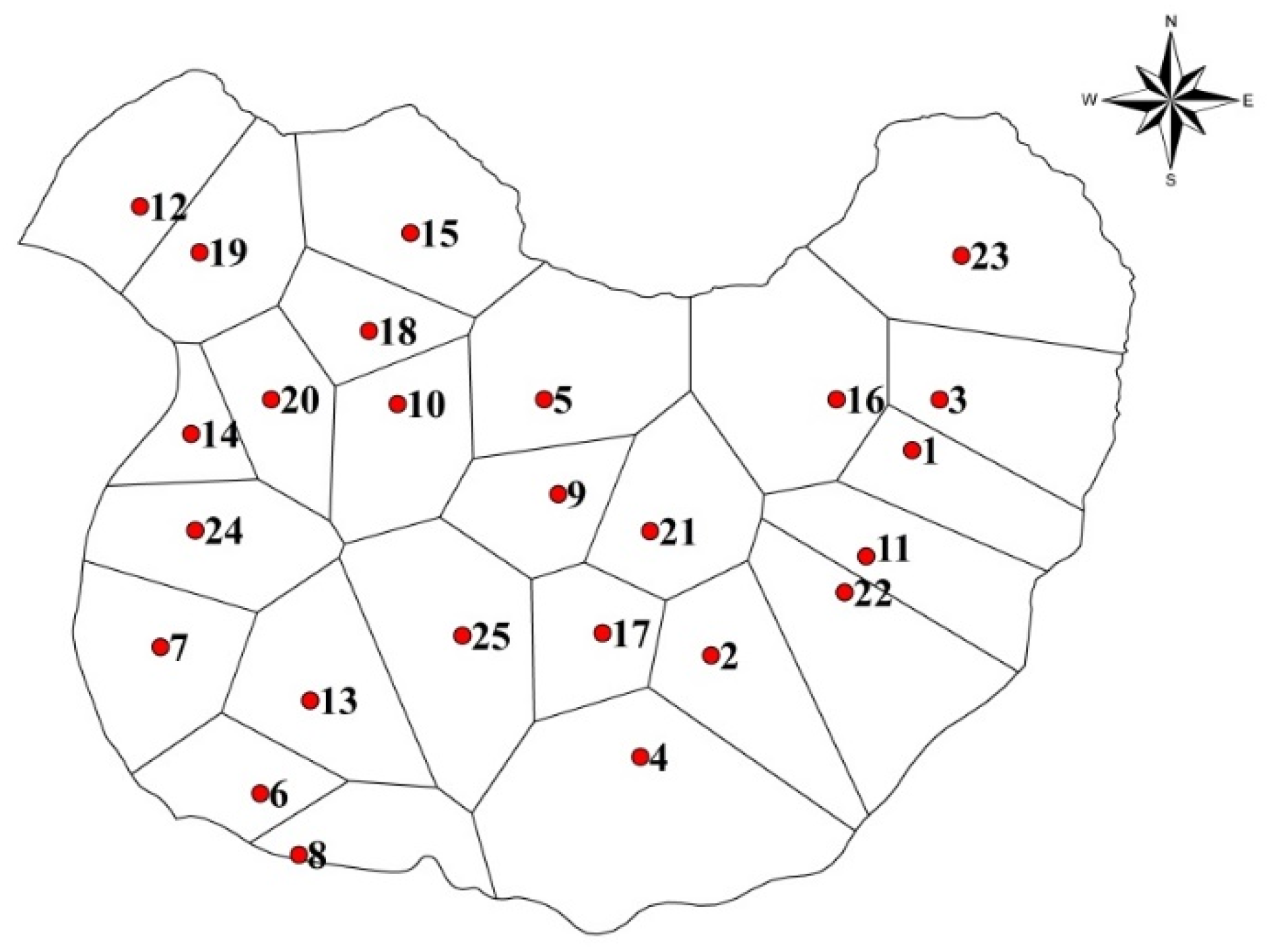
In order to simulate and predict the GWL fluctuations in the Maragheh plain, the monthly averages of rainfall and GWL data were collected from the State Government. The observed precipitation and GWL (Table 1) are available for the years 1996 to 2018 (261 months). The locations of these wells with their Thiessen polygons are shown in Figure 2.

2.3. Completion of Groundwater Level Missing Values

Among 25 observation wells, only 18 wells had complete time series of raw GWL-data during the period 1996 to 2018. The missing values of monthly GWL for seven wells (see Table 2) were estimated by inverse distance weighting (IDW) interpolation. The credibility of the estimated values was checked by comparison with previous month values. Subsequently, the GWL-data were average-weighted using the (25) Thiessen polygon zones to create weight-hydrographs of the GWL-fluctuations (Figure 3).

2.4. Training and Testing of GWL Prediction Models

The ANFIS and Wavelet-ANFIS models were trained based on monthly-observed GWL as well as precipitation (P) data time series. The following input-output prediction model for GWL at time t as a function of GWLt−1 and Ptj was applied:
G W L t = f ( G W L t i , P t j )         f o r       i = 1 , 2 , , n     &   j = 0 , 1 , 2 , , n
i.e., it is assumed that the groundwater levels in month t (GWLt) are correlated with up to t-i previous months ‘groundwater levels and precipitation Ptj. Although Equation (1) is basically just a simple transfer model, it has some physical basis, as groundwater data usually exhibit some persistence, as illustrated in Figure 3, given that groundwater is recharged by rainfall with a delay [40,41].
Autocorrelation analysis of the GWL-time series and cross correlation analysis of the GWL- with the precipitation time series P were performed, respectively. The continuous autocorrelation function Rxx of a time series x is defined as [41]:
R x x = lim T 1 2 T T T x ( t )   x ( t + l ) d t
where T is the period of observation and l is the lag time. For discrete data, Equation (2) is replaced by its discrete homologue which for x = GWL, reads
R G W L , G W L ( m ) = 1 N n = 1 N 1 G W L ( n ) G W L ( l )
where n (=264) is the number of observed months. The cross-correlation function Rxy between two time series x and y is defined similarly to Equations (2) and (3), so that the discrete cross correlation between GWL and P at lag l reads as:
R G W L , P ( m ) = 1 N n = 1 N 1 G W L ( n ) P ( n l )
Figure 4 shows that GWLt is mostly correlated with GWLt−1,t−2,t−3 and Pt−1,t−2,t−3,t−4. Therefore, the final input-output Wavelet-ANFIS and ANFIS and SVM model Equation (1) can be written as:
G W L t = f ( G W L t 1 , G W L t 2 , G W L t 3 ,   P t 1 , P t 2 , P t 3 P t 4 )
For the training and testing of the models the cross-validation method has been used, i.e., the 261-values observed average GWL- and P- data series are divided into a training set of 183 months and testing set of 78 months for prediction with the trained model. Thus, the length of the training data set is 70% and the test (prediction) data makes up the remaining 30%.

2.5. Adaptive Neuro Fuzzy Inference System (ANFIS)

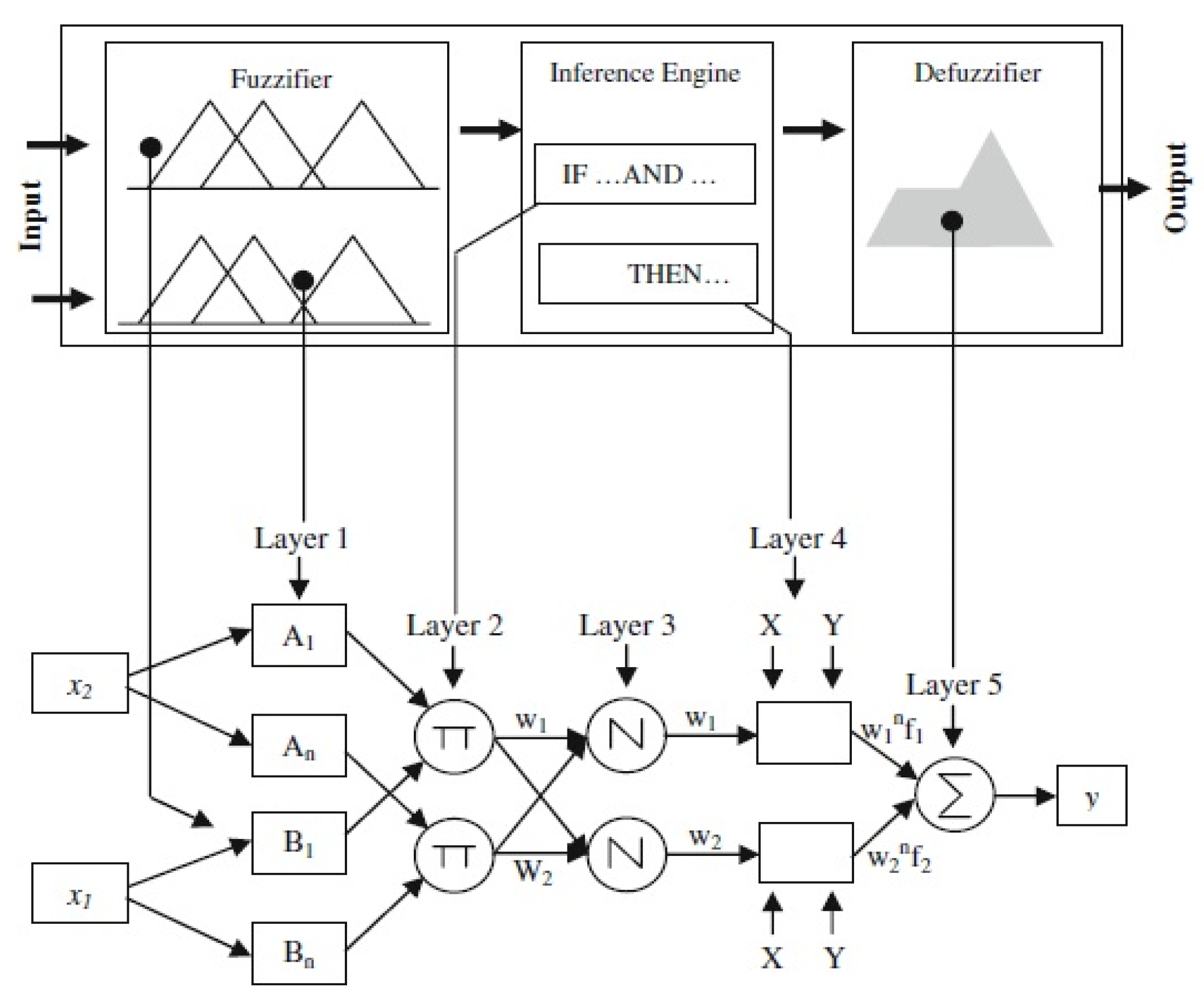
The adaptive neuro fuzzy inference system (ANFIS), first introduced by [13], is a combination of an adaptive neural network and a fuzzy inference system. This model has also an adequate in training, producing and categorizing and has several advantages over classical ANN, such as the capability of handling large amounts of data, dynamic and nonlinear systems modeling, easy use, and efficient computing, while still exhibiting high estimation and prediction accuracies [42]. Combining at the same time the benefits and capabilities of neural network architecture methods and fuzzy logic, ANFIS uses a hybrid approach of the classical gradient descent procedure and systematic back-propagation and thus avoids the “trap” of the error function in a local minimum, typical of the former optimization method [43]. The adaptive network based on the Sugeno fuzzy inference model provides a deterministic system of output equations and is thus a useful approach for parameter estimation [44]. The ANFIS model consists of five layers and is given in Figure 5 [13]. The first layer is called input layer; O1,i is the output of the ith node of the layer 1.
O 1 , i = μ A i ( x 1 ) ,   O 1 , i + 2 = μ B i ( x 2 )   f o r   i = 1 , 2
where X1,2 is the input node i and Ai (or Bi) is a linguistic label associated with this node. Therefore O1,i is the membership grade of a fuzzy set (A1, A2, B1, B2). The second layer consists of rule nodes with AND and/or OR operators. The output (O2,i) is the product of all the incoming signals.
O 2 , i = w i = μ A i ( x 1 ) × μ B i ( x 2 ) ,         f o r   i = 1 , 2
The third layer outputs (O3,i) are called normalized firing strengths.
O 3 , i = w ¯ = w i w 1 + w 2
The fourth layer, called consequent node, is a standard perceptron. Every node i in this layer is an adaptive node with a node function:
O 4 , i = w i n f i = w i n · ( p i x 2 + q i x 2 + r i ) ,   i = 1 , 2
where (pi, qi, ri) is the parameter set of this node; These are referred to as the consequent parameters. Finally, the fifth layer is called the output layer, which computes the overall output as the summation of all incoming signals.
O 5 , i = overall   output = w i ¯ f i =   w i f i w i

2.6. Fuzzy C-Means (FCM) Clustering Method

ANFIS uses neural network training methods and employs fuzzy logic to fit a relationship between some inputs space to output space [13]. The problem with the former is that as the number of inputs increases, the number of rules rises rapidly. In other words, the fuzzy rules increase exponentially [22]. In order to avoid the dimensionality problem in generating too large rule-bases in ANFIS, clustering algorithms are used in FIS models to generate fewer fuzzy rules. It should be noted that clustering methods provide information to obtain initial rules and fuzzy structure for generating the fuzzy inference system [45]. Then, the fuzzy inference system based on these clustering methods can provide a powerful model for establishing relationships between inputs and the output space. The fuzzy C-means (FCM) clustering method was initially introduced by Bezdek in 1973 [46,47] and this approach is known as an improvement and modification of the K-means clustering. In this approach, each data point belongs partly to all clusters, however, with different membership degrees that can vary between 0 and 1. The objective function in the FCM is minimizing the total intra-cluster variance, i.e., the summed square error function within clusters (jm) [48]:
j m ( u , v ) = i = 1 c j = 1 n u i j m d 2 ( x j , v i )
where U = [uij]c×n is the fuzzy partition matrix of c clusters and n data, V = (v1, v2, …, vi) are the centroids of the clusters, uij is the partial membership degree of data xj in cluster i ( 0 u i j 1   &   i = 1 c u i j = 1 ,   2 ,   ,   n ), m is the weighting exponent on each fuzzy membership (which is equal to 2 in this study), xj = (x1, x2, …, xn) is the dataset, vi is the initial value for the cluster center, and d(xj, vi) is the Euclidean distance between the xj data and the cluster center of the ith cluster vi, i.e., xjvi. Equation (11) describes a non-linear optimization problem which can be solved by iterative minimization. The centroid of each cluster is calculated by the partial derivative of Equation (11) with respect to V, then the partial membership degree of data is updated in each iteration by differentiation of the above equation with respect to U:
u i j = ( k = 1 c ( d ( x j , v i ) d ( x j , v k ) ) 2 m 1 ) 1 ,       i = 1 , 2 , , c ;   j = 1 , 2 , , c ;
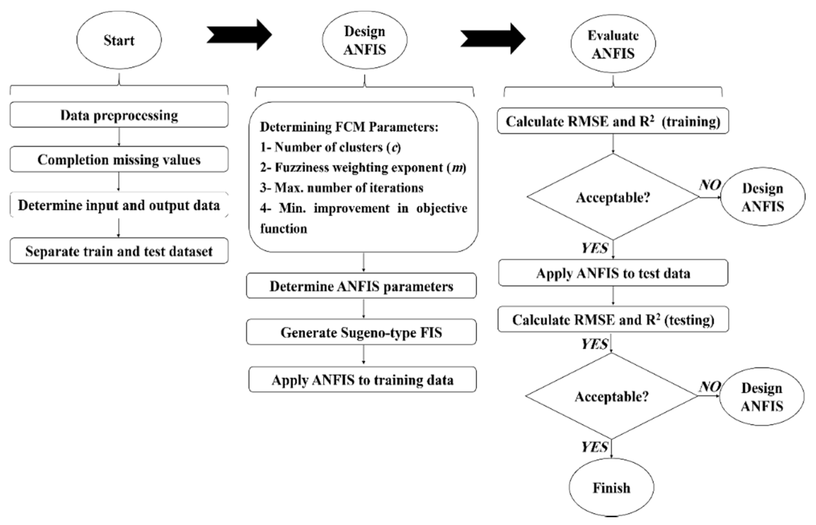
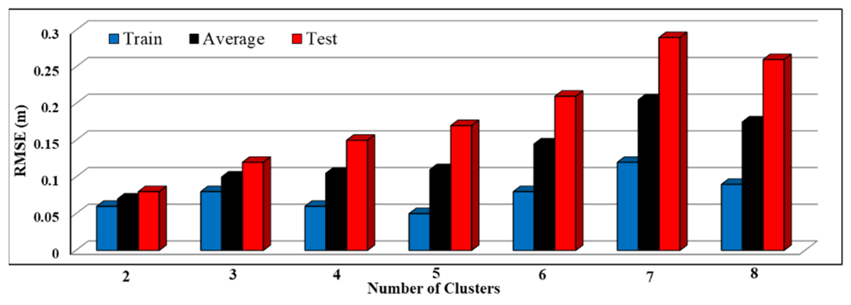
The iteration process is stopped when the variance of intra-clusters in five iterations does not change more than the determined minimum improvement (in this study 10−8), i.e., a minimum improvement in the FCM objective function (convergence) does not occur in five iterations and/or a maximum number of iterations (1000 iterations in this study) is exceeded. In the present study, the FCM algorithm was incorporated into (i.e., coded in) the ANFIS model. The procedure is sketched in Figure 6. The optimal value of the number of clusters was obtained based on trial and error. The RMSE values were calculated for different numbers in the training and test phases (Figure 7). As shown in Figure 7, using two clusters resulted in the least error.

2.7. Wavelet Transformation

The Wavelet Transformation (WT) method is a mathematical tool in Fourier Transform, but seems a more effective tool than the Fourier transform (FT) for studying nonstationary signals [49]. WT is popular because of its multi resolution in time and frequency domain related to temporal data and has been developed to determine information that cannot be easily achieved from raw signals themselves. WT has the ability to consider different aspects of a time series such as trends, discontinuities, and breakpoints [50,51]. In the past, WT was widely used for many hydrological processes including GWL fluctuations, river flow forecast, fault classification or suspended sediments. The continuous wavelet transform (CWT) W(τ,s) of a signal x(t) with respect to a mother wavelet ψ(t) is defined as follows [52]:
W ( τ , s ) =   | s | 1 2 + x ( t ) ψ * ( t τ s ) d t         τ R ,   s R ,   s 0
where τ is the translation parameter, s is the wavelet scale parameter, t is time, and * refers to the complex conjugate. However, the CWT is not often used for forecasting because it requires calculating wavelet coefficients at each scale which means more calculations and, in turn, more compute time. Instead, the discrete wavelet transform (DWT) requires less computation time and is simpler to develop [53]. Discrete wavelets have the following general form [49]:
φ m , n ( t ) = s 0 m 2 ψ ( t n τ 0 s 0 m s 0 m )
where m and n are integers that control the scale and time respectively, τ0 is the location parameter that must be greater than 0, and S0 is a specified fixed dilation step greater than 1. The DWT performs two functions viewed as high-pass and low-pass filters, through which the original time series are passed and then the original time series data are decomposed and divided into two parts, namely “approximation” and “details” [54]. These components explain behavior better and reveal more information about the process than the original time series. Therefore, they can help forecasting models predict with greater accuracy [55,56]. There are many wavelets that can be used as mother wavelets, For the choice of the discrete father-scaling/mother-wavelet filter functions in the DWT/MRA, popular ones are the Haar, the Daubechies wavelet db4 and the irregular wavelet Symlet (sym4), and these are those have been used here [38,57].

2.8. Hybrid Wavelet-ANFIS Model

As shown by [58], a combination of DWT and ANFIS can lead to greater accuracy of GWL prediction. In this regard, after the determination of important parameters, the ANFIS model with the FCM rule generator and the DWT- MRA- decomposed time series of the average GWL and P are integrated to form the Wavelet- ANFIS hybrid model. More specifically, several combinations of different time-lagged GWL- and P- data have been decomposed by haar, Db4, and sym4 data to 1, 2, 3, and 4 levels.

3. Results and Discussion

The performance of the ANFIS and Wavelet-ANFIS models were evaluated by calculating R2 and RMSE statistical parameters. Shown in Table 3, as expected, the performance of the ANFIS model is lower than that of the Wavelet-ANFIS hybrid model, because the Wavelet-ANFIS hybrid model takes advantage of both ANFIS and WT, simultaneously. In particular, WT, or specifically, the DWTMRA, has the ability to consider various aspects of a time series such as trends, discontinuities and breakpoints, and this time-scale localization feature was used to provide decomposition of the input time series up to the 4 levels in the present application, allowing for a separation of the approximation and for providing details of the non-stationary noisy time series, thus enhancing the ANFIS, which uses a combination of fuzzification of the input through membership functions with the network-based algorithm and the use of the hybrid (back propagation tries and gradient descent) optimization method. Table 3 shows the minimum RMSE and the maximum R2 in the training phase with 0.05 and 0.997 and in the test phase as 0.08 and 0.974, respectively, which are obtained with the hybrid wavelet ANFIS model and using the Sym4-mother wavelet (second input combination, Level Decomposition = 3). The best results of the Haar mother wavelets in the test phase has RMSE and R2 values of 0.13 and 0.929, respectively. The db4 mother wavelets also exhibits the best results in the test phase, with corresponding values of 0.09 and 0.968. Comparison of the results of the db4 and sym4 mother wavelets revealed that, although there was no significant difference between the results of these two mother wavelets, the sym4 mother wavelets outperforms db4 mother wavelets slightly. The less accurate results are related to Haar mother wavelets since these are only orthogonal wavelet with a linear phase that cannot provide nonlinear shifts between the original and decomposed signals. By adding the precipitation parameter to the input data, the output accuracy increased in most simulations (on average, 10.2%), although it was more significant in the Wavelet-ANFIS models. In this research, the effect of the decomposition level on the accuracy of the output results of the Wavelet-ANFIS models was investigated. Among the different levels, the decomposition at level 3 had the highest accuracy. However, the accuracy of decomposition level 2 was also acceptable (with only a small difference compared to level 3).
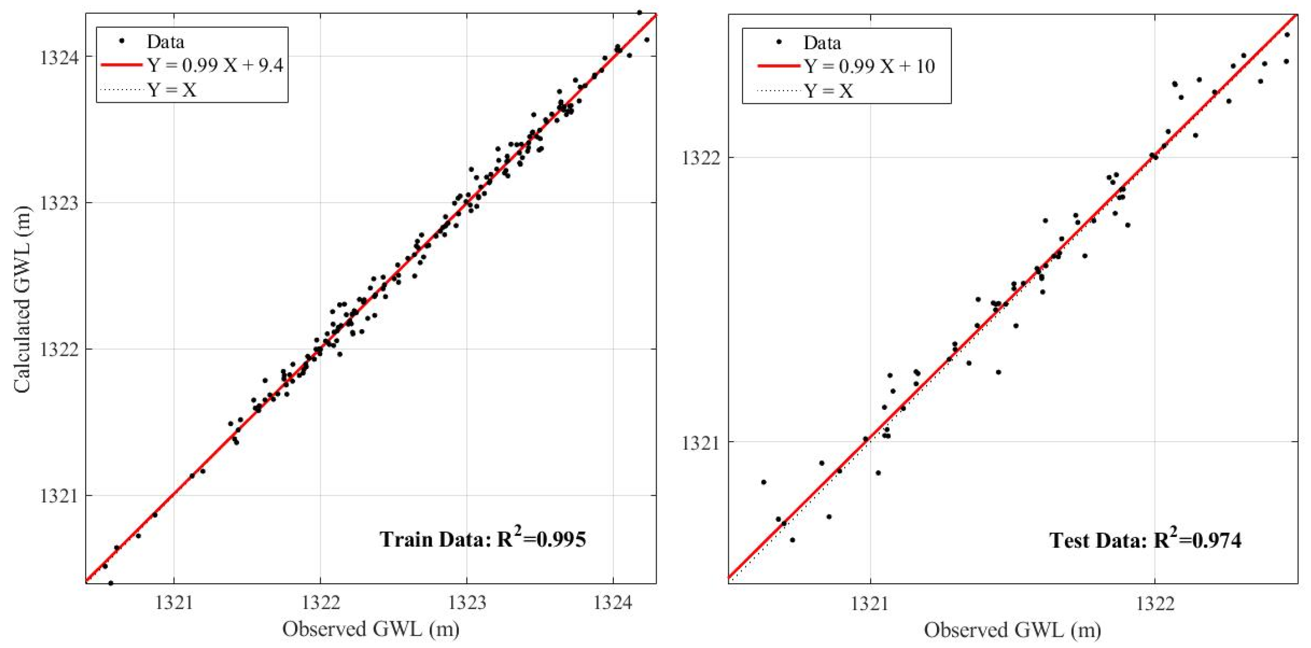
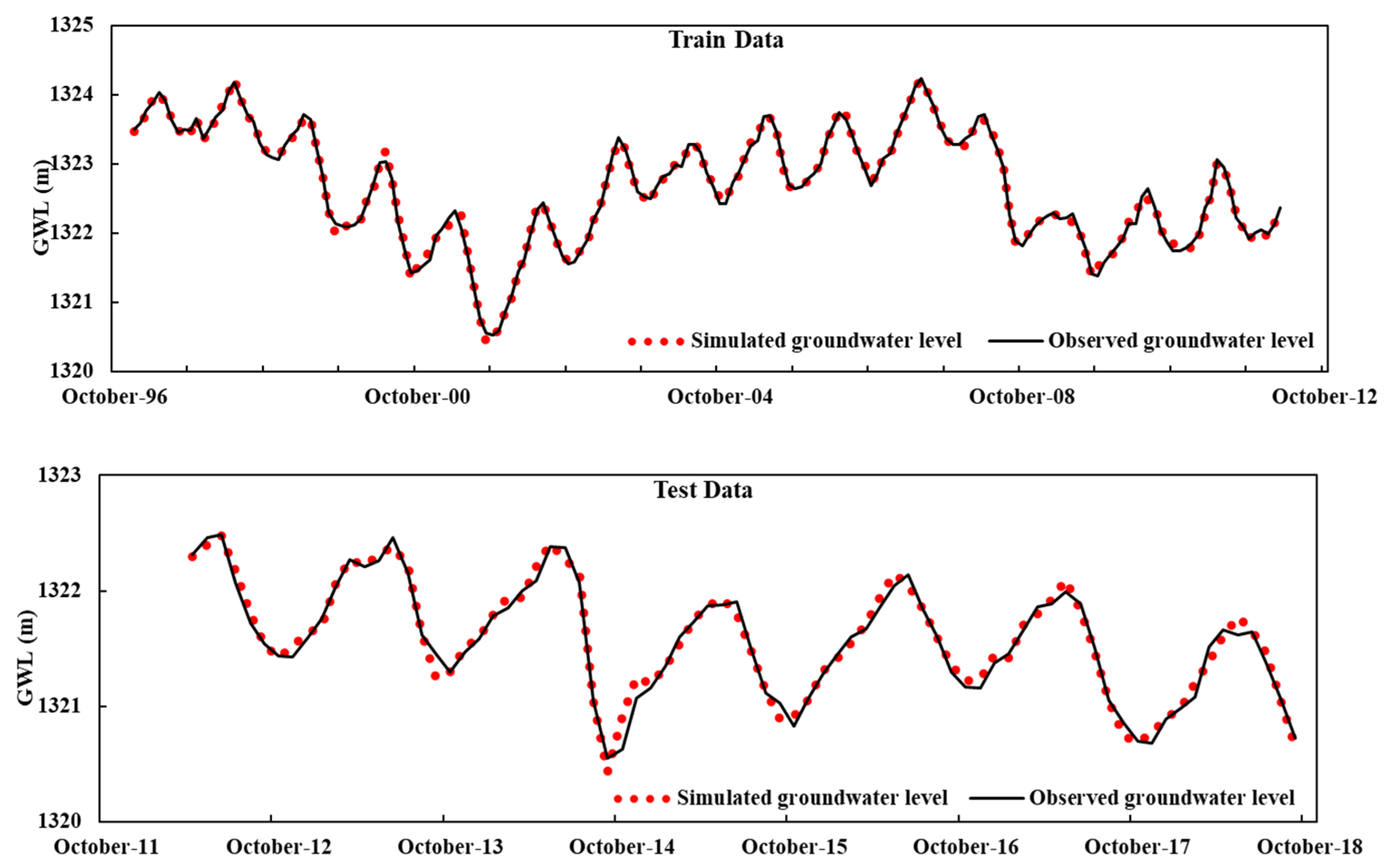
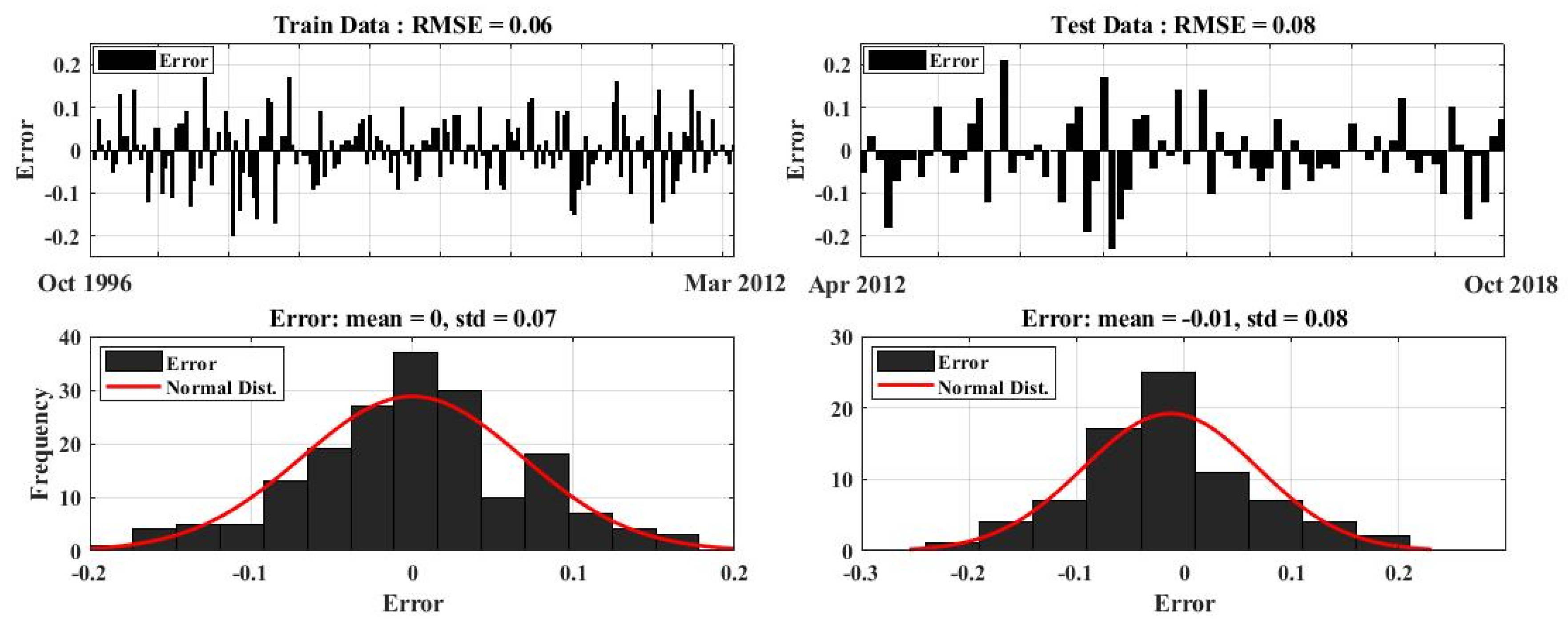
Figure 8 shows the regression plots of the Wavelet-ANFIS-simulated over the observed GWL-data for the training and testing phases and in agreement with the high R2, the points are nearly perfectly lying on the “slope = 1” regression line. The GWL-time series observed and simulated with the best combination of the Wavelet-ANFIS model are presented in Figure 9. There is an acceptable correlation between the observed and simulated GWL data, and the effect of the applied delays on the input data, especially the piezometric head data, is clearly visible. All data-driven prediction methods are based on the idea that the random errors are drawn from a normal distribution and the hybrid Wavelet-ANFIS model is not an exception. Figure 10 illustrates that a-posteriori computed errors of the GWLs predicted with this model, follow indeed a normal distribution.
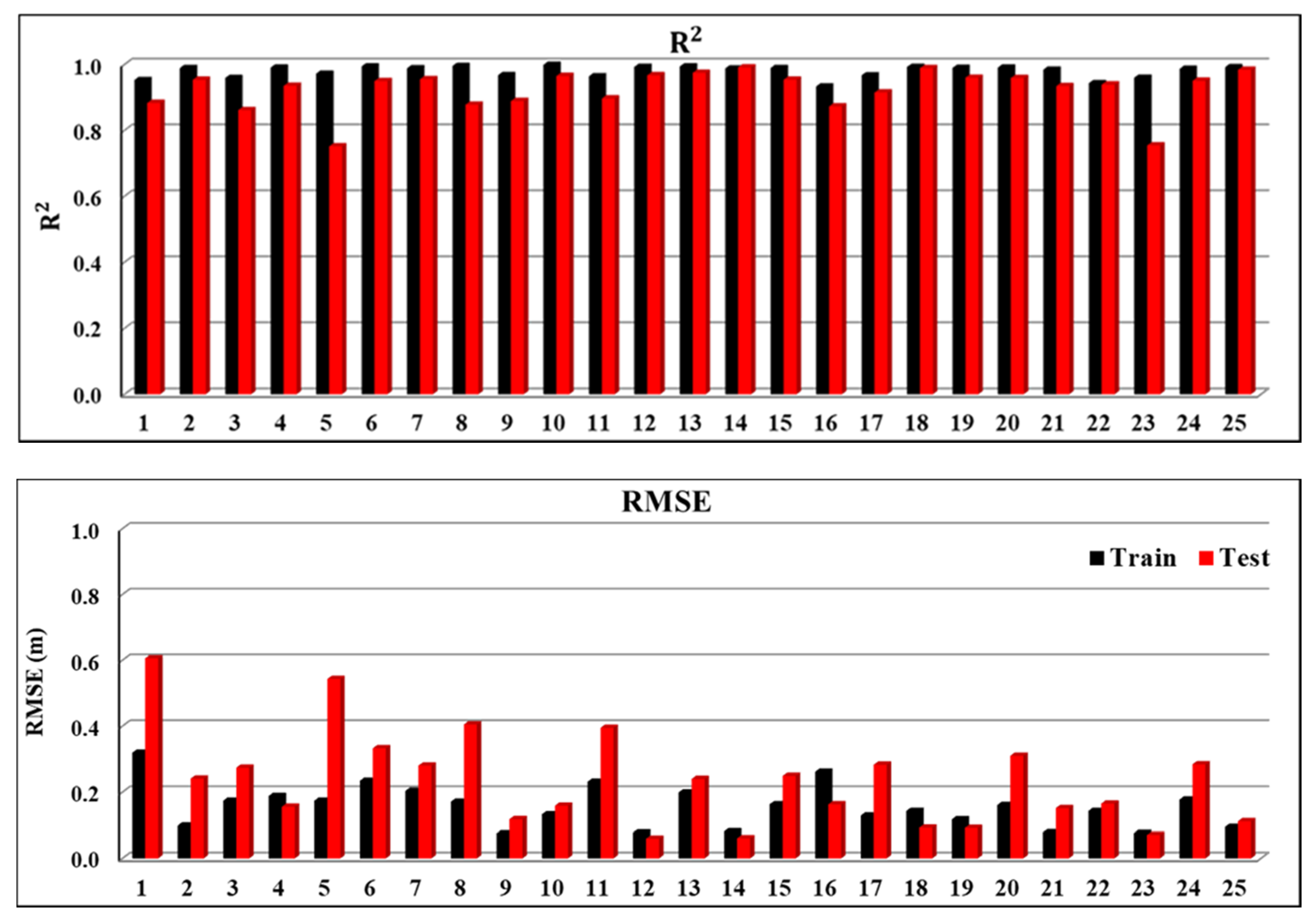
Exceptionally good and reliable predictions of the average GWL of the Maragheh plain using the proposed hybrid wavelet-ANFIS model are evident in all the above presented results. Although the average of GWL is the first and appropriate criterion for the evaluation of the GWL changes all over the plain, in order to understand the spatial variations across the piezometer network in the study plain, the GWL fluctuations in the 25 observation wells were simulated by the hybrid model. The calculated values of R2 and RMSE for both the training and test phase are given in Figure 11. According to most R2 values above 0.95 and most RMSE values less than 0.20 m, especially in the test phase, it can be argued that the model has an acceptable performance in almost all wells.
The results clearly indicate that simulating and predicting a vital parameter of the groundwater budget, namely GWL at time t, can be done accurately using the proposed hybrid model with values of GWL from the previous month and precipitation data as inputs. Although, this is a data driven model, choosing relevant inputs is important because, for example as illustrated in this study, the model considers the groundwater level changes that have a direct relationship with changes in groundwater storage (DS). Furthermore, the difference between volume of precipitation and DS is equal to the sum of other components of the groundwater budget equation, including irrigation water, domestic and industrial demands, as well as natural hydrological processes.

4. Conclusions

This study developed and evaluated hybrid Wavelet-ANFIS models based on the FCM method for groundwater level-(GWL) simulation and prediction, using the Maragheh plain, in northwestern Iran as a case study. In the developed models, GWL were predicted using antecedent GWL-data and precipitation data. A monthly GWL-data series recorded at 25 observation wells during a 22-year period was taken into account. However, given that the GWL data series were not complete, statistical data deficiencies were interpolated using the IDW method. After completing data pre-processing, various statistical analyses were carried out to investigate the time lag correlation of the GWL-time series it was established that that for yielding acceptable simulations of GWL values for a particular month, GWL- and P- data values from 3–4 months prior would be necessary. The 7-time lagged data were used directly as inputs to the ANFIS model to predict GWL, while in the hybrid Wavelet-ANFIS model, the GWL- and P-time series were decomposed to level 4 by means of DWT-MRA.
The performance of the developed hybrid model was examined at four decomposition levels. Input data were divided into two parts: one for simulation (training) and the other for prediction (testing) phases. Thus, in this study, the length of the training data set is 70% and the test (prediction) data makes up the remaining 30%. The best values of RMSE and R2 were obtained 0.05 m and 0.997, respectively, in the training phase and of 0.08 m and 0.974 the testing (prediction) phase, which indicates that the hybrid Wavelet-ANFIS using the Symlet mother wavelet and decomposition level 3 performs best. According to the results of the hybrid Wavelet-ANFIS model, the model performance was acceptable in estimating GWL fluctuations all over the plain, such that the difference between the observed and simulated values was negligible, meaning the incorporation of the wavelet transforms in ANFIS increased the performance of ANFIS model, especially in the prediction phase. Another noteworthy characteristic of this coupled model in the simulated and predicted values of GWL fluctuations is the use of the FCM clustering method which generates fewer fuzzy rules, thereby overcoming the well-known data dimensionality problem.
Finally, it can be argued that the Wavelet-ANFIS-FCM-clustering model in terms of performance, especially, when, due to a lack of data, all physical processes such as surface-groundwater interactions, are not completely understood, presents an attractive method and reliable tool for groundwater level prediction under different water resources management scenarios. Nonetheless, there is a need to further evaluate the developed model in other regions or in the same plain but with different GWL- and P-time series.

Author Contributions

Conceptualization, H.O. and M.Z.; methodology, M.Z.; software, M.M.J.; validation, H.O., M.M.J. and M.Z.; writing—original draft preparation, M.M.J. and H.O.; writing—review and editing, G.J.-P.S.; supervision, H.O., G.J.-P.S. and M.Z. All authors have read and agreed to the published version of the manuscript.

Funding

The time and effort of M.Z. was supported by the Luxembourg National Research Fund (FNR) in the framework of an industrial fellowship with Ref. No. 14111453.

Institutional Review Board Statement

Not applicable.

Informed Consent Statement

Not applicable.

Data Availability Statement

Data available on request. The data presented in this study are available on request from the first author (M.M.J.). The ground water data in Iran are not publicly available but can be requested from respective water authorities.

Conflicts of Interest

The authors declare no conflict of interest.

References

  1. Koch, M. Challenges for future sustainable water resources management in the face of climate change. In Proceedings of the 1st NPRU Academic Conference, Nakhon Pathom University, Nakhon Pathom, Thailand, 23–24 October 2008. [Google Scholar]
  2. Nayak, P.; SatyajiRao, Y.; Sudheer, K. Groundwater level forcasting in a shallow aquifer using artificial neural network. J. Water Resour. Manag. 2006, 20, 77–90. [Google Scholar] [CrossRef]
  3. Jolly, I.D.; McEwan, K.L.; Holland, K.L. A review of groundwater–surface water interactions in arid/semiarid wetlands and the consequences of salinity for wetland ecology. Ecohydrology 2008, 1, 43–58. [Google Scholar] [CrossRef]
  4. Prinos, S.T.; Lietz, A.C.; Irvin, R.B. Design of a real-time groundwater level monitoring network and portrayal of hydrologic data in Southern Florida. In USGC Water Resources Investigations Report; Geological Survey (US): Reston, WV, USA, 2002. [Google Scholar]
  5. Lijun, F.; Shuquan, L. Forecasting the runoff using least square support vector machine. Tianjin Teach. Comm. 2007, TJGL06-099, 884–889. [Google Scholar]
  6. Nourani, V.; Alami, M.T.; Aminfar, M.H. Combined neural—Wavelet model for prediction of Ligvanchayi watershed precipitation. Eng. Appl. Artif. Intell. 2009, 22, 466–472. [Google Scholar] [CrossRef]
  7. Behzad, M.; Asghari, K.; Coppola, E.J.R. Comparative study of SVMs and ANNs in aquifer water level prediction. J. Comput. Civ. Eng. 2010, 24, 408–413. [Google Scholar] [CrossRef]
  8. Yoon, H.; Jun, S.C.; Hyun, Y.; Bae, G.O.; Lee, K.K. A comparative study of artificial neural networks and support vector machines for predicting groundwater levels in a coastal aquifer. J. Hydrol. 2011, 396, 128–138. [Google Scholar] [CrossRef]
  9. Shiri, J.; Kisi, O.; Yoon, H.; Lee, K.-K.; Hossein Nazemi, A. Predicting groundwater level fluctuations with meteorological effect implications—A comparative study among soft computing techniques. Comput. Geosci. 2013, 56, 32–44. [Google Scholar] [CrossRef]
  10. Mirzavand, M.; Khoshnevisan, B.; Shamshirband, S.; Kisi, O.; Ahmad, R.; Akib, S. Evaluating groundwater level fluctuation by support vector regression and neuro fuzzy methods: A comparative study. Nat. Hazards 2015, 102, 1611–1612. [Google Scholar] [CrossRef]
  11. Zare, M.; Koch, M. Groundwater level fluctuations simulation and prediction by ANFIS- and hybrid Wavelet-ANFIS/Fuzzy C-Means (FCM) clustering models: Application to the Miandarband plain. J. Hydro-Environ. Res. 2018, 18, 63–76. [Google Scholar] [CrossRef]
  12. Srivastav, R.K.; Sudheer, K.P.; Chaubey, I. A simplified approach to quantifying predictive and parametric uncertainty in artificial neural network hydrologic models. Water Resour. Res. 2007, 43. [Google Scholar] [CrossRef] [Green Version]
  13. Jang, J.S.R. ANFIS: Adaptive-network-based fuzzy inference system. IEEE Trans. Syst. Man Cybern. 1993, 23, 665–685. [Google Scholar] [CrossRef]
  14. Shiri, J.; Kisi, O. Comparison of genetic programming with neuro-fuzzy systems for predicting short-term water table depth fluctuations. Comput. Geosci. 2011, 37, 1692–1701. [Google Scholar] [CrossRef]
  15. Amutha, R.; Porchelvan, P. Seasonal prediction of groundwater levels using ANFIS and radial basis neural network. Int. J. Geol. Earth Environ. Sci. 2011, 1, 98–108. [Google Scholar]
  16. Moosavi, V.; Vafakhah, M.; Shirmohammadi, B.; Ranjbar, M. Optimization of Wavelet-ANFIS and Wavelet-ANN Hybrid Models by Taguchi Method for Groundwater Level Forecasting. Arab. J. Sci. Eng. 2014, 39, 1785–1796. [Google Scholar] [CrossRef]
  17. Wen, X.; Feng, Q.; Yu, H.; Wu, J.; Si, J.; Chang, Z.; Xi, H. Wavelet and adaptive neuro-fuzzy inference system conjunction model for groundwater level predicting in a coastal aquifer. Neural. Comput. Appl. 2015, 26, 1203–1215. [Google Scholar] [CrossRef]
  18. Emamgholizadeh, S.; Moslemi, K.; Karami, G.H. Prediction the groundwater level of Bastam Plain (Iran) by Artificial Neural Network (ANN) and Adaptive Neuro-Fuzzy Inference System (ANFIS). Water Resour. Manag. 2014, 28, 5433–5446. [Google Scholar] [CrossRef]
  19. Khaki, M.; Yusoff, I.; Islami, N. Application of the Artificial Neural Network and Neuro-fuzzy System for Assessment of Groundwater Quality. Clean Soil Air Water. 2014, 42, 1–10. [Google Scholar] [CrossRef]
  20. Rajaee, T.; Ebrahimi, H.; Nourani, V. A review of the artificial intelligence methods in groundwater level modeling. J. Hydrol. 2019, 572, 336–351. [Google Scholar] [CrossRef]
  21. Zare, M.; Koch, M. Using ANN and ANFIS Models for simulating and predicting groundwater level fluctuations in the Miandarband Plain, Iran. In Proceedings of the 4th IAHR Europe Congress, Liege, Belgium, 27–29 July 2016; pp. 416–423. [Google Scholar]
  22. Vaidhehi, V. The role of Dataset in training ANFIS system for course Advisor. Int. J. Innov. Res. Adv. Eng. 2014, 1, 249–253. [Google Scholar]
  23. Mirrashid, M. Earthquake magnitude prediction by adaptive neuro-fuzzy inference system (ANFIS) based on fuzzy C-means algorithm. Nat. Hazards 2014, 74, 1577–1593. [Google Scholar] [CrossRef]
  24. Kuczera, G. Uncorrelated measurement error in flood frequency inference. Water Resour. Res. 1992, 28, 183–188. [Google Scholar] [CrossRef]
  25. Sang, Y.F.; Wang, D.; Wu, J.C.; Zhu, Q.P.; Wang, L. The relation between periods’ identification and noises in hydrologic series data. J. Hydrol. 2009, 368, 165–177. [Google Scholar] [CrossRef]
  26. Donoho, D.H. De-noising by soft-thresholding. IEEE Trans. Inform. Theory 1995, 41, 613–617. [Google Scholar] [CrossRef] [Green Version]
  27. Elshorbagy, A.; Simonovic, S.P.; Panu, U.S. Noise reduction in chaotic hydrologic time series: Facts and doubts. J. Hydrol. 2002, 256, 147–165. [Google Scholar] [CrossRef]
  28. Torrence, C.; Compo, G.P. A practical guide to wavelet analysis. Bull. Am. Meteorol. 1998, 79, 61–78. [Google Scholar] [CrossRef] [Green Version]
  29. Jansen, M. Minimum risk thresholds for data with heavy noise. IEEE Signal Process. Lett. 2006, 13, 296–299. [Google Scholar] [CrossRef]
  30. Nourani, V.; Hosseini Baghanam, A.; Adamowski, J.; Kisi, O. Applications of hybrid wavelet–Artificial intelligence models in hydrology: A review. J. Hydrol. 2014, 514, 358–377. [Google Scholar] [CrossRef]
  31. Nourani, V.; Alami, M.T.; Daneshvar Vousoughi, F. Wavelet-entropy data pre-processing approach for ANN-based groundwater level modeling. J. Hydrol. 2015, 524, 255–269. [Google Scholar] [CrossRef]
  32. Ebrahimi, H.; Rajaee, T. Simulation of groundwater level variations using wavelet combined with neural network, linear regression and support vector machine. Glob. Planet. Chang. 2016, 148, 181–191. [Google Scholar] [CrossRef]
  33. Barzegar, R.; Fijani, E.; Asghari Moghaddama, A.; Tziritis, E. Forecasting of groundwater level fluctuations using ensemble hybrid multi-wavelet neural network-based models. Sci. Total Environ. 2017, 599–600, 20–31. [Google Scholar] [CrossRef]
  34. Malekzadeh, M.; Kardar, S.; Saeb, K.; Shabanlou, S.; Taghavi, L. A novel approach for prediction of monthly ground water level using a hybrid wavelet and non-tuned self-adaptive machine learning model. Water Resour. Manag. 2019, 33, 1609–1628. [Google Scholar] [CrossRef]
  35. Shirmohammadi, B.; Moradi, H.; Moosavi, V.; Semiromi, M.T.; Zeinali, A. Forecasting of meteorological drought using Wavelet-ANFIS hybrid model for different time steps (case study: Southeastern part of east Azerbaijan province, Iran). Nat. Hazards 2013, 69, 389–402. [Google Scholar] [CrossRef]
  36. Shafaei, M.; Kisi, O. Lake Level Forecasting Using Wavelet-SVR, Wavelet-ANFIS and Wavelet-ARMA Conjunction Models. Water Resour. Manage. 2015, 30, 79–97. [Google Scholar] [CrossRef]
  37. Karthika, B.S.; Deka, P.C. Prediction of air temperature by hybridized model (Wavelet-ANFIS) using wavelet decomposed data. Aquat. Procedia 2015, 4, 1155–1161. [Google Scholar] [CrossRef]
  38. Moosavi, V.; Vafakhah, M.; Shirmohammadi, B.; Behnia, N. A Wavelet-ANFIS hybrid model for groundwater level forecasting for different prediction periods. Water Resour. Manag. 2013, 27, 1301–1321. [Google Scholar] [CrossRef]
  39. Sang, Y.F.; Wang, D.; Wu, J.C.; Zhu, Q.P.; Wang, L. Entropy-based wavelet de-noising method for time series analysis. Entropy 2009, 11, 1123–1147. [Google Scholar] [CrossRef] [Green Version]
  40. Markovic, D.; Koch, M. Stream response to precipitation variability: A spectral view based on analysis and modelling of hydrological cycle components. Hydrol. Process. 2015, 29, 1806–1816. [Google Scholar] [CrossRef]
  41. Zhang, Y.-K.; Li, Z. Temporal scaling of hydraulic head fluctuations: Nonstationary spectral analyses and numerical simulations. Water Resour. Res. 2005, 41, 7–10. [Google Scholar] [CrossRef]
  42. Jang, J.S.R.; Sun, C.T.; Mizutani, E. Neuro-Fuzzy and Soft Computing: A Computational Approach to Learning and Machine Intelligence; Prentice Hall: Upper Saddle River, NJ, USA, 1997. [Google Scholar]
  43. Tahmasebi, P.; Hezarkhani, A. A hybrid neural networks-fuzzy logic-genetic algorithm for grade estimation. Comput. Geosci. 2012, 42, 18–27. [Google Scholar] [CrossRef] [Green Version]
  44. Takagi, T.; Sugeno, M. Fuzzy identification of systems and its applications to modeling and control. In IEEE Transactions on Systems Man and Cybernetics; IEEE: Piscataway, NJ, USA, 1985; pp. 116–132. [Google Scholar]
  45. Cobaner, M. Evapotranspiration estimation by two different neuro-fuzzy inference systems. J. Hydrol. 2011, 398, 292–302. [Google Scholar] [CrossRef]
  46. Bezdek, J. Cluster validity with fuzzy sets. J. Cybern. 1973, 3, 58–73. [Google Scholar] [CrossRef]
  47. Bezdek, J.C. Pattern Recognition with Fuzzy Objective Function Algorithms; Plenum Press: New York, NY, USA, 1981; pp. 1–256. [Google Scholar]
  48. Ayvaz, M.T.; Karahan, H.; Aral, M.M. Aquifer parameter and zone structure estimation using kernel-based fuzzy c-means clustering and genetic algorithm. J. Hydrol. 2007, 343, 240–253. [Google Scholar] [CrossRef]
  49. Grossman, A.; Morlet, J. Decompositions of hardy functions into square integrable wavelets of constant shape. Siam J. Math. Anal. 1984, 15, 723–736. [Google Scholar] [CrossRef]
  50. Adamowski, J.; Sun, K. Development of a coupled wavelet transform and neural network method for flow forecasting of non-perennial rivers in semi-arid watersheds. J. Hydrol. 2010, 390, 85–91. [Google Scholar] [CrossRef]
  51. Singh, R.M. Wavelet-ANN model for flood events. In Proceedings of the International Conference on Soft Computing for Problem Solving (SocProS 2011), Springer India, Roorkee, India, 20–22 December 2011; pp. 165–175. [Google Scholar]
  52. Partal, T. River flow forecasting using different artificial neural network algorithms and wavelet transform. Can. J. Civ. Eng. 2009, 36, 26–38. [Google Scholar] [CrossRef]
  53. Adamowski, J.; Fung Chan, H. A wavelet neural network conjunction model for groundwater level forecasting. J. Hydrol. 2011, 407, 28–40. [Google Scholar] [CrossRef]
  54. Kisi, O.; Cimen, M. A wavelet-support vector machine conjunction model for monthly streamflow forecasting. J. Hydrol. 2011, 399, 132–140. [Google Scholar] [CrossRef]
  55. Catalão, J.P.S.; Pousinho, H.M.I.; Mendes, V.M.F. Hybrid wavelet-PSO-ANFIS approach for short-term electricity prices forecasting. IEEE Trans. Power Syst. 2011, 26, 137–144. [Google Scholar] [CrossRef]
  56. Remesan, R.; Bray, M.; Shamim, M.A.; Han, D. Rainfall-runoff modelling using a wavelet-based hybrid SVM scheme. Hydroinformatics in hydrology, hydrogeology and water resources. In Proceedings of the Symposium JS.4 at the Joint Convention of the International Association of Hydrological Sciences (IAHS) and the International Association of Hydrogeologists (IAH), Hyderabad, India, 6–12 September 2009; pp. 41–50. [Google Scholar]
  57. Mallat, S.G. A theory for multiresolution signal decomposition: The wavelet representation. IEEE Trans. Pattern Anal. Mach. Intell. 1989, 11, 674–693. [Google Scholar] [CrossRef] [Green Version]
  58. Nourani, V.; Alami, M.T.; Daneshvar Vosoughi, F. Hybrid of SOM-clustering method and wavelet-anfis approach to model and infill missing groundwater level data. J. Hydrol. Eng. 2016, 21, 05016018. [Google Scholar] [CrossRef]
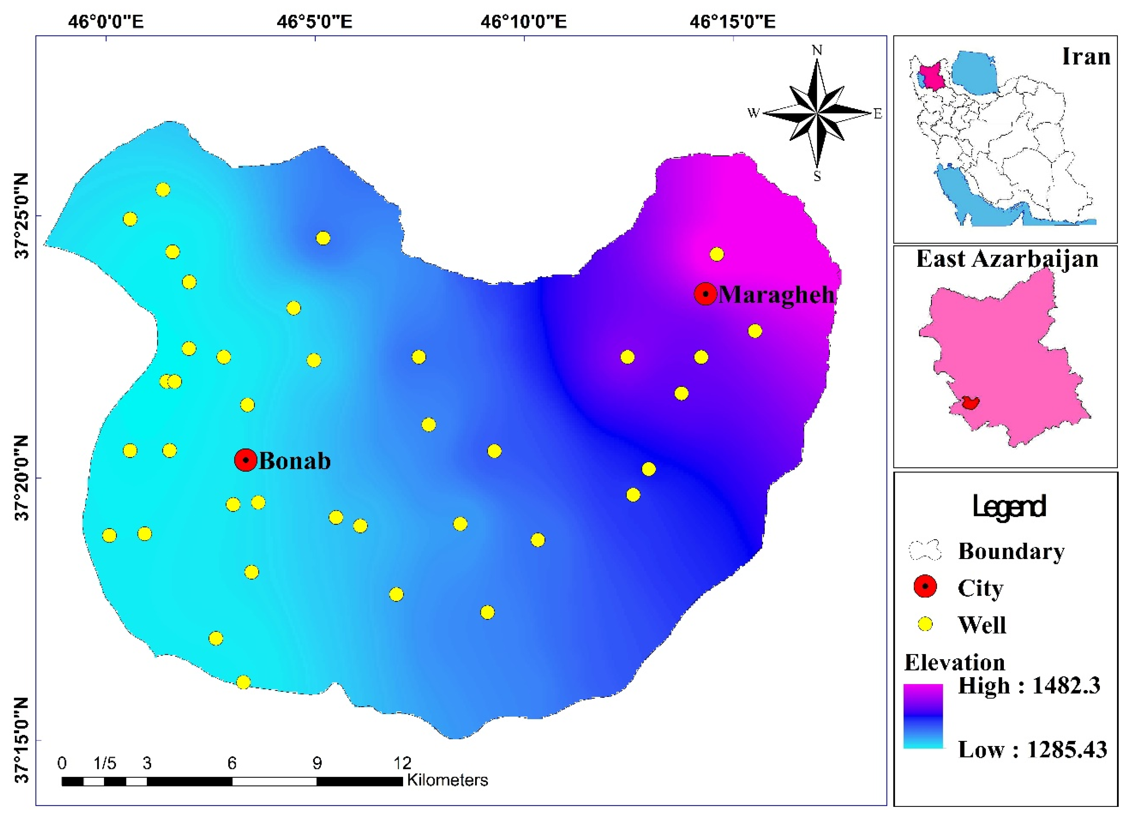
Figure 1. The Maragheh plain in northwestern Iran.
Atmosphere 12 00009 g001
Figure 2. Borehole locations with Thiessen polygons.
Atmosphere 12 00009 g002
Figure 3. Average groundwater level (GWL) fluctuations in the Maragheh plain during 1996–2018.
Atmosphere 12 00009 g003
Figure 4. Autocorrelation function for GWL (a) and cross correlation function between GL and Precipitation (b).
Atmosphere 12 00009 g004
Figure 5. Architecture of ANFIS [11].
Atmosphere 12 00009 g005
Figure 6. Flow diagram of the combination of fuzzy c-means clustering (FCM) method and ANFIS [11].
Atmosphere 12 00009 g006
Figure 7. The values of RMSE for different number of clusters in the FCM method.
Atmosphere 12 00009 g007
Figure 8. Regression plots of Wavelet-ANFIS (Sym4 mother wavelet)-simulated over observed GWL-data for training (left panel) and testing (right) phases.
Atmosphere 12 00009 g008
Figure 9. Wavelet-ANFIS/Sym4-simulated and observed GWL-time series for the training (upper panel) and testing (lower panel) phases.
Atmosphere 12 00009 g009
Figure 10. Distribution of the GWL-random errors of the wavelet-ANFIS model.
Atmosphere 12 00009 g010
Figure 11. Results of GWL-simulation in all 25 wells (see Figure 2).
Atmosphere 12 00009 g011
Table 1. List of the 25 wells and the areas of their Theissen polygons.
IDLocationA(ha)Elevation(m)IDLocationA(ha)Elevation(m)
1Seraju (khoshkbarchi)11941397.214Akhond gheshlagh6501280.58
2Sezavar mousavi1659133115Alghou20991336.31
3Varjouy18011404.816Pahr abad22431413.41
4Yengi kand khoushe mehr36941327.9217Khoushe mehr10071314.25
5Rousht bozorg istgahe rah ahan20961337.8918Rousht kouchak9211296.26
6Khaneh bargh ghadim9311287.0119Bonab energy atomi15271280.25
7Gharah chopogh behdasht15531285.0920Bonab mantagheh abiyari10891282.14
8Khalilvand rouberouye ajorpazi9981286.8221Jadeh sarj baghal kanal14541345.71
9Maragheh foroudgah10941325.2322Khanghah ghabrestan21261359.17
10Zavasht ghabrestan14161297.923Maragheh khajeh nasir32511474.24
11Varjouy maleki14651371.9924Bonab aval rah darya15291284.25
12Khezerlou shourgol16451284.425Chelghay masjed22851305.22
13Zavaregh bimarestan17061292.36----
Table 2. Number of missing values for wells with missing data.
Well ID381012182024
Number of Missing Values171627173075
Table 3. Results of the various model combinations of input data with the optimum number of clusters (c = 2) for the training and testing phases of ANFIS.
MethodDecomposition LevelANFIS InputsTrainingTesting
RMSE(m)R2RMSE(m)R2
ANFIS-GLt−1,GLt−2,GLt−30.160.9620.190.870
Wavelet-ANFIS/haar1-0.110.9830.140.923
2-0.110.9830.140.921
3-0.100.9840.190.878
4-0.110.9830.160.891
Wavelet-ANFIS/db41-0.090.9870.130.949
2-0.070.9920.110.964
3-0.070.9950.080.972
4-0.060.9960.140.921
Wavelet-ANFIS/sym41-0.100.9510.140.933
2-0.080.990.120.955
3-0.060.9940.090.969
4-0.060.9940.090.966
ANFIS-GLt−1,GLt−2,GLt−3,Pt−1,Pt−2,Pt−3,Pt−40.130.9750.180.878
-----
Wavelet-ANFIS/haar1-0.090.9880.160.891
2-0.090.9880.130.927
3-0.090.9880.130.929
4-0.090.9880.130.925
Wavelet-ANFIS/db41-0.080.9910.120.949
2-0.070.9940.090.967
3-0.060.9960.090.968
4-0.060.9970.10.959
Wavelet-ANFIS/sym41-0.080.990.130.931
2-0.070.9930.110.954
3-0.060.9950.080.974
4-0.050.9960.080.974
Publisher’s Note: MDPI stays neutral with regard to jurisdictional claims in published maps and institutional affiliations.