1. Introduction
The importance of accurate weather forecasting at high resolution is widely recognized, since atmospheric phenomena have significant impacts on human life. Availability of meteorological information results is strategic when aimed at managing adverse events. Accurate forecasts can also support many different strategic economic sectors, such as power supply from renewable energy, tourism, agriculture, flood, civil protection and river transport, i.e., whenever numerical weather prediction (NWP) models are fundamental to providing a detailed forecast in a short time range. Moreover, very high resolution NWP can be used to provide forecast products in time and space within localized areas subject to high impact atmospheric events. In order to define the kind of products required, it is essential to perform a long and detailed calibration of NWP models using different observation platforms and a spatial and temporal resolution similar to the model. Very high resolution NWP models are powerful tools that allow for a more detailed representation of orography, sea–land interaction and soil–atmosphere interface (due to the availability of soil moisture data) relative to models with resolution in the range of 7–10 km. This feature is expected to improve the capability to represent very localized events. Moreover, these high-resolution models require less parameterization, e.g., deep convection is explicitly solved.
More specifically, in southern Italy severe weather events are generally connected to deep convection, leading to intense precipitation and strong winds. When a limited-area model is run at a spatial resolution on the order of 10 km, the formation and propagation of these convective systems are poorly simulated because the model relies on parameterized convection without describing the interaction between the convective scale and the larger scale. With recent advances in computing power, studies have increasingly shown improvements in model performance when the grid spacing is increased to 1 km and the parameterization of deep convection is switched off (i.e., convection-permitting). Moreover, high resolution leads to significant advantages in representing orographic regions, producing high-order statistics and predicting events with small temporal and spatial scales [
1]. This approach reveals extensive capability [
2], especially when surface forcing, such as land use and land/sea contrast, play a significant role in controlling convection triggering. However, such models must be run over relatively small areas nested in coarser resolution models (e.g., [
3,
4]) that do not represent convection explicitly.
In recent years, several studies have been performed to analyze the potential benefits provided by the high resolution. Baldauf et al. [
5] analyzed results of the operational NWP COSMO at convective scale (2.8 km) and performed related sensitivity activity. They found that the system was able to predict deep convection explicitly, providing an improved precipitation forecast when compared to coarser NWP models. The dynamic core was based on an accurate and efficient Runge–Kutta solver.
Heppelmann et al. [
6] evaluated NWP forecasts provided by both COSMO and ICON against wind mast observations, finding that both models were affected by shortcomings regarding the representation of the diurnal cycle. In particular, for the summer, nocturnal wind speed results were underestimated. Uzan et al. [
7] tested the accuracy of planetary boundary layer (PBL) height estimations from COSMO, based on the bulk Richardson method over Israel, finding the model was characterized by good accuracy in both flat and elevated terrain. They concluded that a combination of ceilometers (devices that use a laser to determine the height of a cloud ceiling) and high-resolution model data enabled generation of a corrected spatial evolution of the daytime PBL height over Israel.
The feasibility of calibrating COSMO at about 3 km resolution using an objective multivariate calibration method built on a quadratic metamodel (MM) was investigated by Voudouri et al. [
8]. This metamodel makes a calibration by sampling the parameter space and then fitting a continuous quadratic regression. In this way, it was possible to reproduce the forecasted field for any parameter combination. This methodology was applied by Voudouri et al. [
9] for model calibration over the domain, which included Switzerland and Northern Italy at 2 km resolution.
The Italian Aerospace Research Center (CIRA), as a member of the COSMO Consortium, developed a specific convective-scale model configuration with horizontal resolution of about 1 km, running daily (currently only for research purposes) over an area including part of the Campania and Lazio regions (southern Italy). The main reason was the assessment of a specific configuration for this geographical area, having a low number of sensitivity tests with the COSMO model. The optimization of the configuration was performed through a tuning procedure [
10], aimed at selecting the parameters that have been shown to play a significant role in determining model response [
11]. In fact, the COSMO formulation includes several parameterization schemes [
12,
13], which account statistically for the effects of phenomena that are not described by the governing equations or that occur at unresolved scales.
The main aim of this work is to test the capabilities of the COSMO model in reproducing the main atmospheric variables at the CIRA site, by exploiting the technical instrumentation available in situ. In fact, CIRA has developed a weather situational awareness system (WSAS) [
14], able to provide real-time data for updating mission management and trajectory generation functions; it includes the Meteo Service Center, a ground segment that processes and integrates observational data from the instrumentation installed. Moreover, to avoid the limitation of analysis related to a single point, evaluation is also conducted against daily observational data in different locations. Radio sounding data available at Pratica di Mare (Roma) are also considered. Even with the limitations due to the consideration of a limited number of locations, we believe that this study represents a step forward, since only a few studies have been conducted to evaluate an NWP using a combination of different kinds of observations; the majority of studies are based only on ground observations. A five-month period was considered in order to allow the possibilities of testing the model over different seasons and different climate features (winter and spring).
The paper is organized as follows:
Section 2 contains a description of the model set-up and of observations. In
Section 3, results are presented and discussed. Concluding remarks are presented in
Section 4.
2. The COSMO Model and Observational Data
The limited area model used in the present work as an NWP tool is COSMO, a non-hydrostatic dynamic downscaling model for three-dimensional compressible flows [
15]. It is developed by the European consortium COSMO (COnsortium for Small-scale MOdeling). The atmosphere is considered as an ideal mixture of dry air, water vapor, liquid and solid water, subject to the gravity and to the Coriolis forces [
16].
The governing equations are discretized on a rotated latitude longitude grid, assuming terrain-following coordinates in the vertical, and using finite difference techniques. Time integration is performed using a fixed time step, with different algorithms of integrations (Leapfrog, Runge–Kutta). The unresolved scale phenomena are treated in a statistical manner through a number of parameterizations of grid- and sub-grid scale physical phenomena, such as convection, radiation, land–atmosphere interaction, turbulence and microphysics. For each scheme, input parameters appearing as constants or exponents must be specified. The model version used in this work is the cosmo5.05, released in 2018.
2.1. Simulation Set-Up
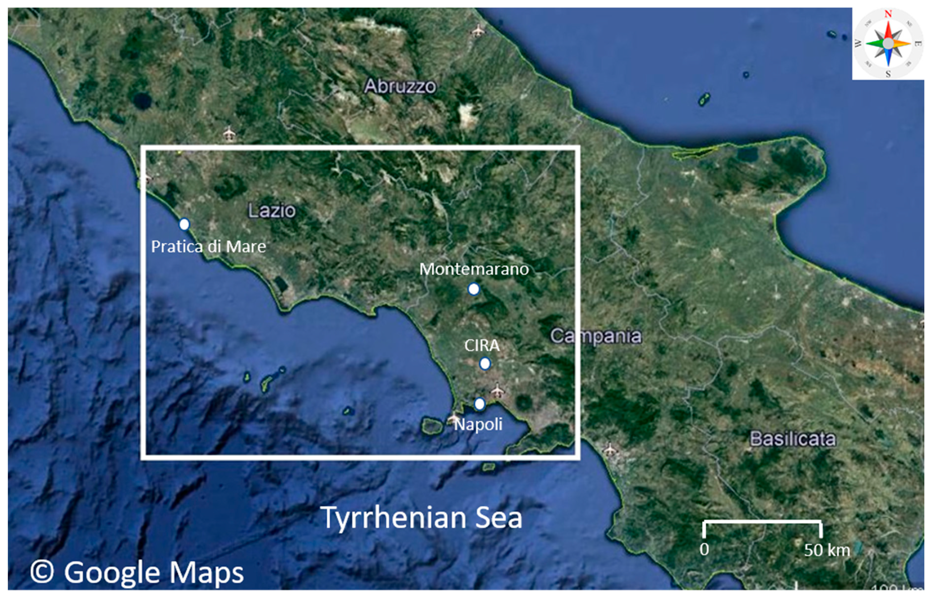
The simulated domain (12.22°–14.55° E; 40.63°–41.88° N) is shown in
Figure 1. It extends for about 260 km in the longitude and 138 km in latitude direction and covers the northern part of the Campania region and the southern part of Lazio. This domain has a mild climate influenced by the sea and a colder internal zone characterized by the presence of mountains. High precipitation values are recorded, even along the coasts, generally up to 1000 mm/year since most of the region is exposed to the humid westerly winds. Extreme meteorological events frequently affect this area, with very intense and localized precipitation events and strong winds. This is likely associated with the increased Mediterranean temperature, especially from the Tyrrhenian Sea, where storm cells are generated.
The spatial resolution was set to 0.009° (about 1 km), leading to a domain with 260 × 138 points, while the number of vertical levels was 60. The time step was equal to 10 s. Initial and boundary conditions were provided by the ECMWF IFS global model [
3], characterized by a spatial resolution of 0.075° (about 8.5 km). The boundary conditions were updated every 3 h. Numerical simulations (duration: 24 h each) were performed daily assuming a 6 h spin-up period for each day, in accordance with [
17]. COSMO has run at CIRA since September 2017; however, in this work models were evaluated from January 2018 (because the current model version was installed at this time) until May 2018 in order to have a 5 month period sufficient for covering two seasons (winter and spring) and different climate features. As reported in [
18], in most of the Mediterranean region, convective overshoot cloud are more frequent in summer and autumn than in winter and spring, with frequencies larger than 1.3‰; therefore, if the sea surface temperature is relatively warm, it can provide enough moisture to support localized convection [
19].
The model configuration was derived from MeteoSwiss for daily operational simulations at very high resolution (about 1 km). This configuration was calibrated over the domain considered in this work by changing the values of some parameters according to the sensitivity tests described in [
10]. As stated by Beven in [
20], the parameters must be set properly in order to guarantee that the main features of the real domains are properly reflected in the model. Deep convection was explicitly solved as required, while shallow convection was parameterized by means of the Tiedtke scheme [
21]. Optimization included parameters related to microphysics, radiation, vertical turbulent diffusion, soil and vegetation processes. Specifically, better results in terms of temperature can be achieved for this domain by setting the parameter controlling vertical variation for the critical relative humidity in the sub-grid cloud formation to a minimum (uc1). This is defined empirically to compute the rate of cloud cover. Cloud formation is evaluated using physical functions that depend on relative humidity levels at which clouds are expected to form [
22]. Further improvements are obtained by choosing the minimum value for the laminar resistance to heat (rlam_heat). This regulates the heat resistance length of the laminar layer so that a larger resistance of the laminar layer to heat transfer corresponds to higher values [
23], and this was introduced to consider the complexity of the interaction between the atmosphere and the surface. Benefits are also obtained by reducing the minimal diffusion coefficient for heat (tkhmin), which controls the minimum value for the turbulence coefficient for heat [
24]. This configuration offers a good improvement in terms of temperature bias (reduced up to 0.5 °C) over this complex orographic area. Finally, internal turbulence switches were set in order to better reproduce the scheme based on the diagnostic turbulence closure [
25]. This scheme adopts diffusion coefficients for momentum and heat (coupling turbulent fluxes with vertical gradients), which are determined in terms of wind shear and thermal stability.
2.2. Observational Data
The model was evaluated against a combination of observational data. The CIRA meteorological ground station uses Vaisala MAWS301. This is a robust system that provides quality-controlled data in applications including synoptical observation, meteorology, hydrology and aviation weather. Every minute it provides the 2 m temperature, precipitation, pressure and relative humidity. A Vaisala LAP-3000 Doppler beam swinging wind profiler is installed at CIRA (property of ARPAC, Environmental Protection Agency of Campania Region) that reliably provides vertical profiles for the wind speed and direction from a height of 120 m up to 3 km above ground level every 30 min, with a spatial resolution of about 50 m. An optional extended antenna aperture improves the performance by narrowing the beam width, thereby increasing the antenna gain and reducing side lobes. The CIRA ceilometer CS135 is a lidar sensor able to measure the cloud height, the cloud cover and the backscatter profile. Such measurements are made in the troposphere between 0 and 10 km, every 30 s. It is equipped with a diode laser that emits short impulses in the vertical direction, at a wavelength of 905 nm and frequency of 10 kHz. Using a sample frequency of 30 Mhz provides a vertical resolution of 5 m. The backscatter profiles were used to evaluate the mixing layer height (MLH) through a MATLAB code [
26]. MLH represents the vertical extension of mixing due to thermal and mechanical turbulence inside the planetary boundary layer.
Furthermore, an evaluation was performed against radio sounding data collected daily in Pratica di Mare (12.45°–41.67°) by CNMCA (Centro Nazionale di Meteorologia e Climatologia Aeronautica) at hours 00 and 12, in terms of vertical profiles of temperature and dew point. A radiosonde is a battery-powered telemetry instrument carried into the atmosphere by a weather balloon that measures various atmospheric parameters and transmits them by radio to a ground receiver. Radiosounding is a key part of the atmospheric observation system since it is able to provide accurate data on vertical profiles for temperature, humidity and winds.
Finally, daily temperature, precipitation and wind data from stations at Napoli Capodichino airport and Montemarano were considered in order to validate the model at different locations, respectively, close to the sea (Napoli) and on a hill (Montemarano). These data were provided by the SCIA (Sistema nazionale per l’elaborazione e diffusione di dati climatici) system (national system for the collection, elaboration, and diffusion of climate data) developed by ISPRA (Istituto Superiore Protezione e Ricerca Ambientale) [
27].
3. Results
The model evaluated several variables: temperature and precipitation represent the basic weather variables; wind speed and direction were considered due to their importance in relation to power supply and renewable energies; clouds and planetary boundary layer (PBL) height were measured because they are important not only for weather forecasts, but also for air pollution analysis.
Standard indices for performance evaluation were used [
28]: mean bias (BIAS) and root-mean-square error (RMSE):
Here,
Si and
Oi are, respectively, the simulated and observed values at the
i-th time step;
N is the total number of time steps considered. BIAS provides the average error, its value being affected by the possibility of error compensation. RMSE provides the average magnitude error without indicating the sign of the deviation, which has the disadvantage of putting more influence on larger errors than smaller ones. As pointed out in some works (e.g., [
29]), RMSE is not appropriate because it can vary with the average error and with the variability within the error distribution.
Moreover, the index of agreement (
d) proposed by Willmott [
30] has been considered:
A value of 1 indicates a perfect match, while 0 indicates no agreement at all. The index of agreement can detect additive and proportional differences in the observed and simulated means and variances; however, d is highly sensitive to extreme values since it measures squared differences. Further, CORR (spatial correlation between simulated and observed values) and STD_RATIO (ratio between model and observation standard deviations) were used. All analyses were conducted over the 137 days included in the period 15 January–31 May 2018. In all figures, 15 January is marked with 1, and so on, until the last day (31 May) marked with 137.
3.1. Temperature Analysis
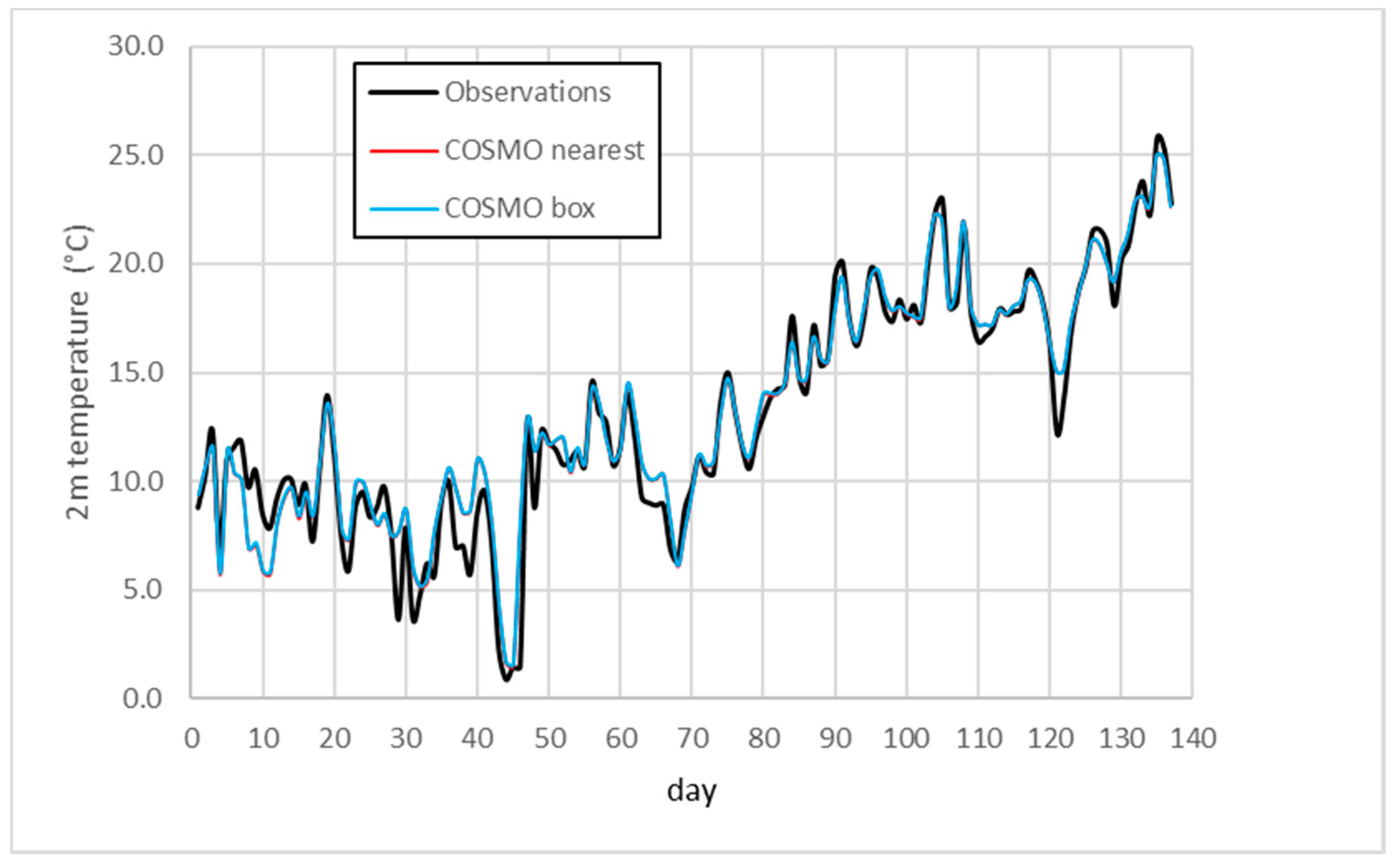
The first analysis compared 2 m temperature values (t2m) recorded by the CIRA weather station with the model data, considering values related to the nearest grid point and average values over a 3 × 3 grid box.
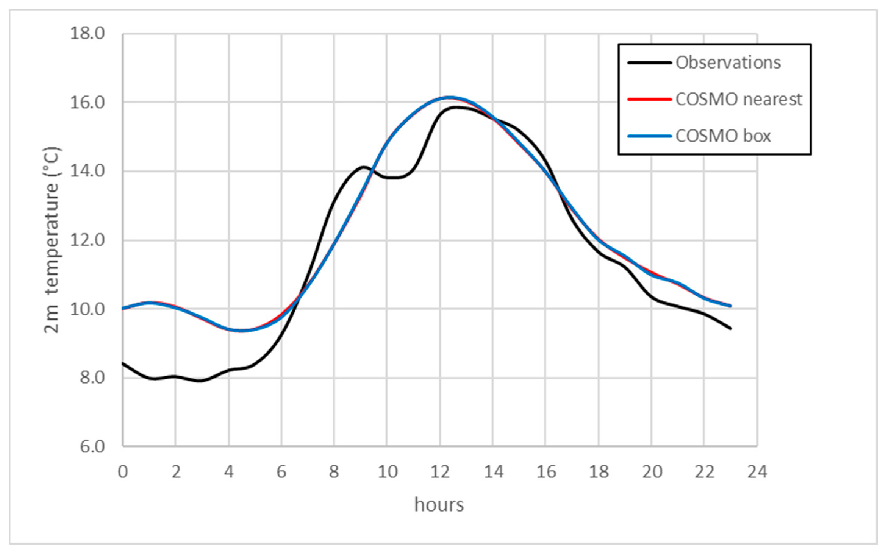
Figure 2 shows the average hourly daily values (observed and simulated) over the entire period considered. The graph highlights no significant differences between the nearest and grid box values. The comparison showed the model was capable of reproducing daily temperature values, with a sight tendency for underestimation. An analysis of the diurnal cycle (
Figure 3) (obtained by averaging data over the entire period) revealed good performances, even at the hourly scale, especially for maximum daily values. On the other hand, minimum nocturnal values were generally underestimated. A possible explanation is that the model uses a Biosphere-Atmosphere Transfer Scheme (BATS) [
31], and the simulated bare soil evaporation by BATS may be too high, thus creating a bias towards moist and cold conditions, particularly during night time. Tests conducted over the selected periods in [
32] revealed that small improvements could be achieved by using a resistance-based formulation (RB) scheme [
33]. The average values of BIAS, RMSE and
d over the entire period considered were evaluated (
Table 1) and revealed good performances, even though there were obvious bias compensation effects: a non-negligible, positive bias (6.6 °C) affected the simulation on 1 March, when a sudden temperature increase (about 11 °C) was recorded over 24 h, and the model was not able to reproduce this sharp jump; a large, negative bias was recorded in winter on 23 January, due to relevant underestimations in nocturnal hours. In order to validate the model in different locations, model data were compared with observations at Napoli Capodichino airport and Montemarano.
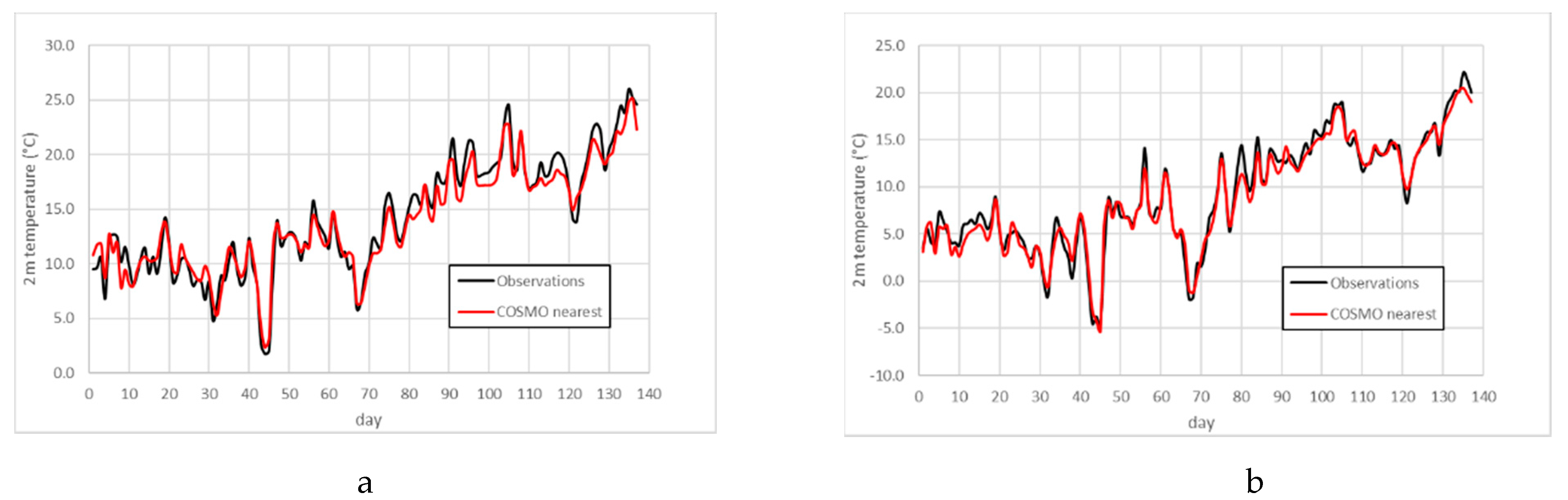
Figure 4 shows the daily values (observed and simulated) over the entire period considered. In Napoli, from January to March the model accurately reproduced t2m, while in April and May both daily minimum and maximum values were generally underestimated. Since this station is located in an urban environment, this underestimation could be due to the unsuitable representation of cities and suggests the need for specific urban parameterization [
34]. In Montemarano, the figure shows the model adequately reproduced the observed series, with some underestimation of daily maximum values. The good performance in both locations was confirmed by the numerical values shown in
Table 1.
3.2. Precipitation Analysis
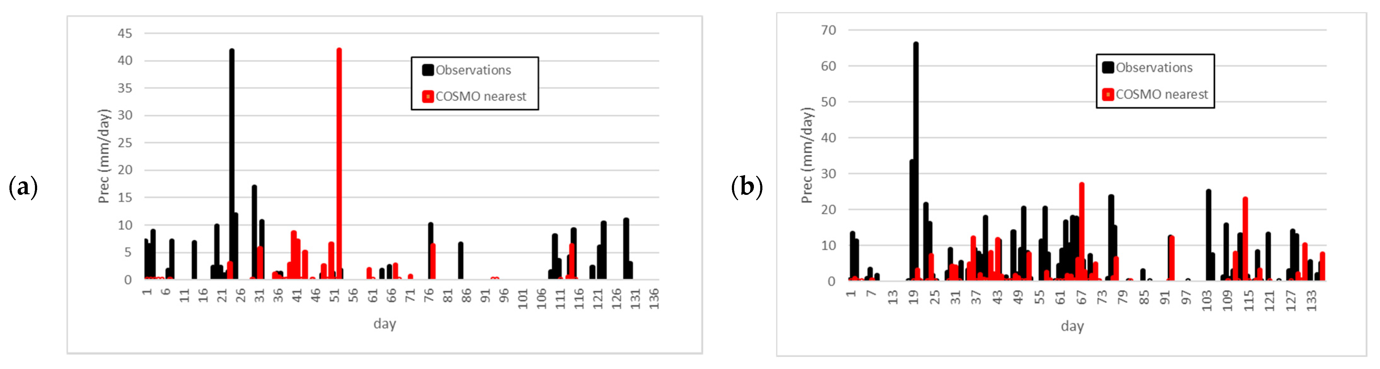
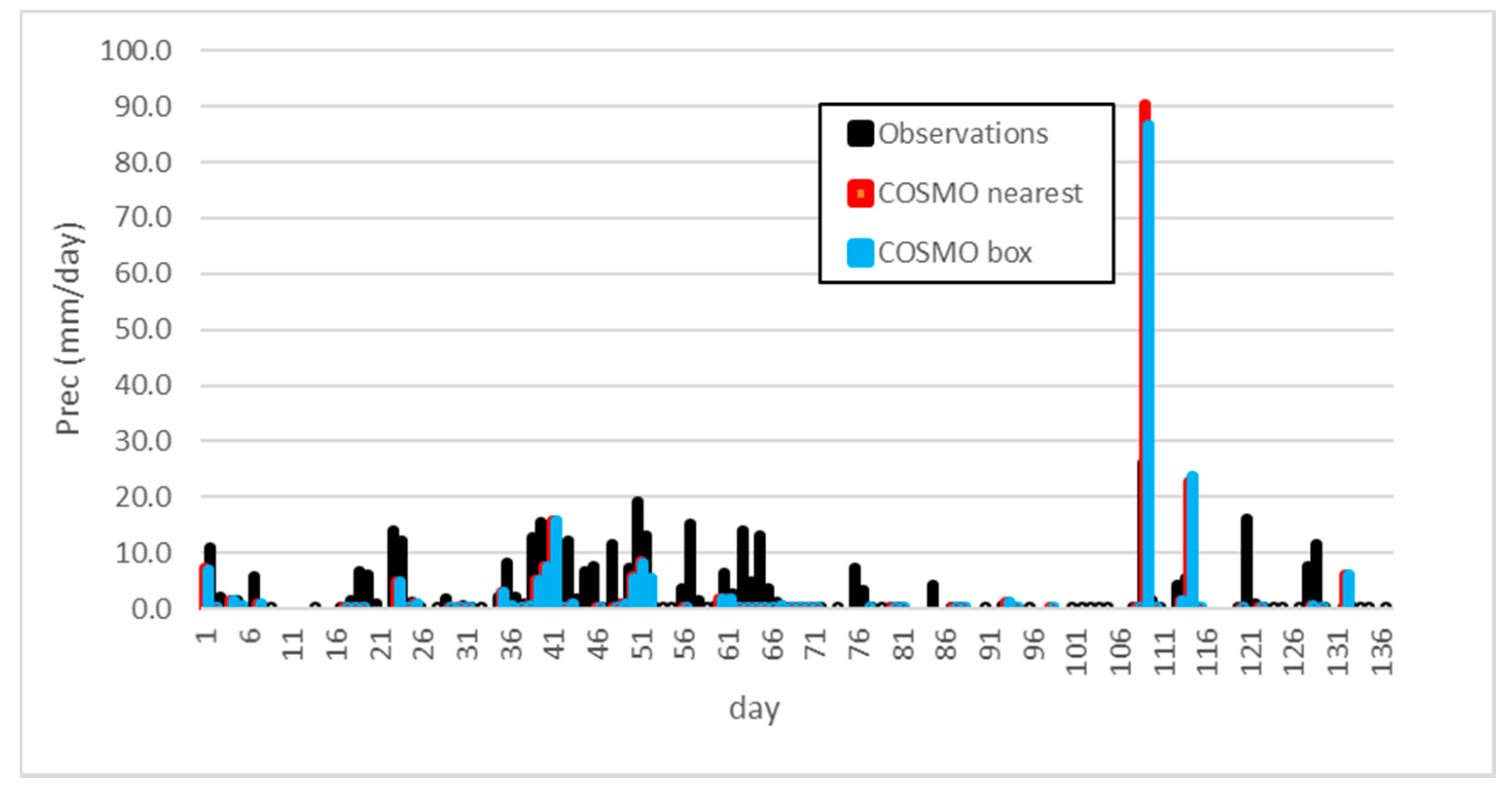
The second analysis involved daily precipitation values at CIRA weather station.
Figure 5 shows a histogram of the observed and simulated (nearest point and grid box) values over the period considered. As for temperature, there were no differences between nearest and grid box values. The histogram reveals that the model was able to reproduce dry days (precipitation less than 1 mm), while the model generally underestimated the rainy days (with the exception of a few cases). In more detail, the model’s ability to reproduce the number of rainy days was investigated by using a contingency table (
Table 2), considering an “event” as a day in which precipitation was larger than 1 mm.
Table 3 contains the numerical values of these quantities over the observed period. These values confirmed that the model adequately reproduced the dry days (correct negatives: 77 out of 137), while a strong underestimation of rainy days was confirmed. In addition, the critical success index (CSI), defined as the ratio of events correctly forecasted, was quite low and was calculated as follows:
Further analyses were performed in order to investigate the origin of these shortcomings. It is known that COSMO experiences difficulties when localizing rain events. Strong precipitation is often simulated in geographical areas away from where the event really takes place. As shown in [
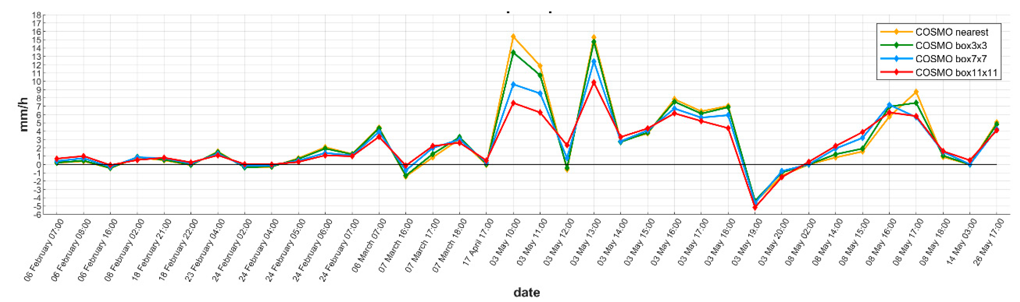
35], discrepancies between COSMO and observed precipitation intensities are caused primarily by temporal and spatial shifts in the simulated precipitation patterns. In the present work, we investigated the dependency of the simulated values on the size of the box considered. Besides the 3 × 3 size, we also examined larger boxes, namely 7 × 7 and 11 × 11.
Figure 6 shows hourly precipitation biases for the selected days and hours with different boxes, revealing that the use of larger boxes leads to better representation of precipitation for days in which precipitation was overestimated (e.g., 3 May 2018, 11:00).
Overall, the model inadequately simulated some climate features of the area considered, and there was internal variability and some deficiencies in the lateral boundary conditions. Further investigations were conducted comparing model data with observations in Napoli Capodichino airport and Montemarano.
Figure 7 shows a histogram of daily observed and simulated (nearest point) values. Similar to what was observed at CIRA, the model adequately reproduced dry days in both locations, while it underestimated precipitation on rainy days at the hill station (Montemarano). On the other hand, precipitation was overestimated in Napoli in February, probably due to sea surface temperature biases in proximity to the sea. In spite of the convection permitting scheme adopted, the model still had problems in simulating convective precipitation, which is typical in spring months, so further adjustments to the configurations are needed. Improvements in this area can be achieved by setting the laminar heat resistance factor to the minimum value. Increasing the vertical velocity factor of snow also provides a positive effect on precipitation and will be the object of further investigation.
3.3. Wind Analysis
This evaluation was conducted assuming data provided by the Wind Profiler as observational reference. This instrument is installed at CIRA, but it is owned by ARPAC; data are provided to CIRA in the spirit of cooperation between the institutions. Evaluations were performed considering the COSMO grid point closest to the Wind Profiler location. Wind intensity values in the vertical directions were interpolated to the Wind Profiler height levels, while for the direction, model height values closest to the observed ones were considered.
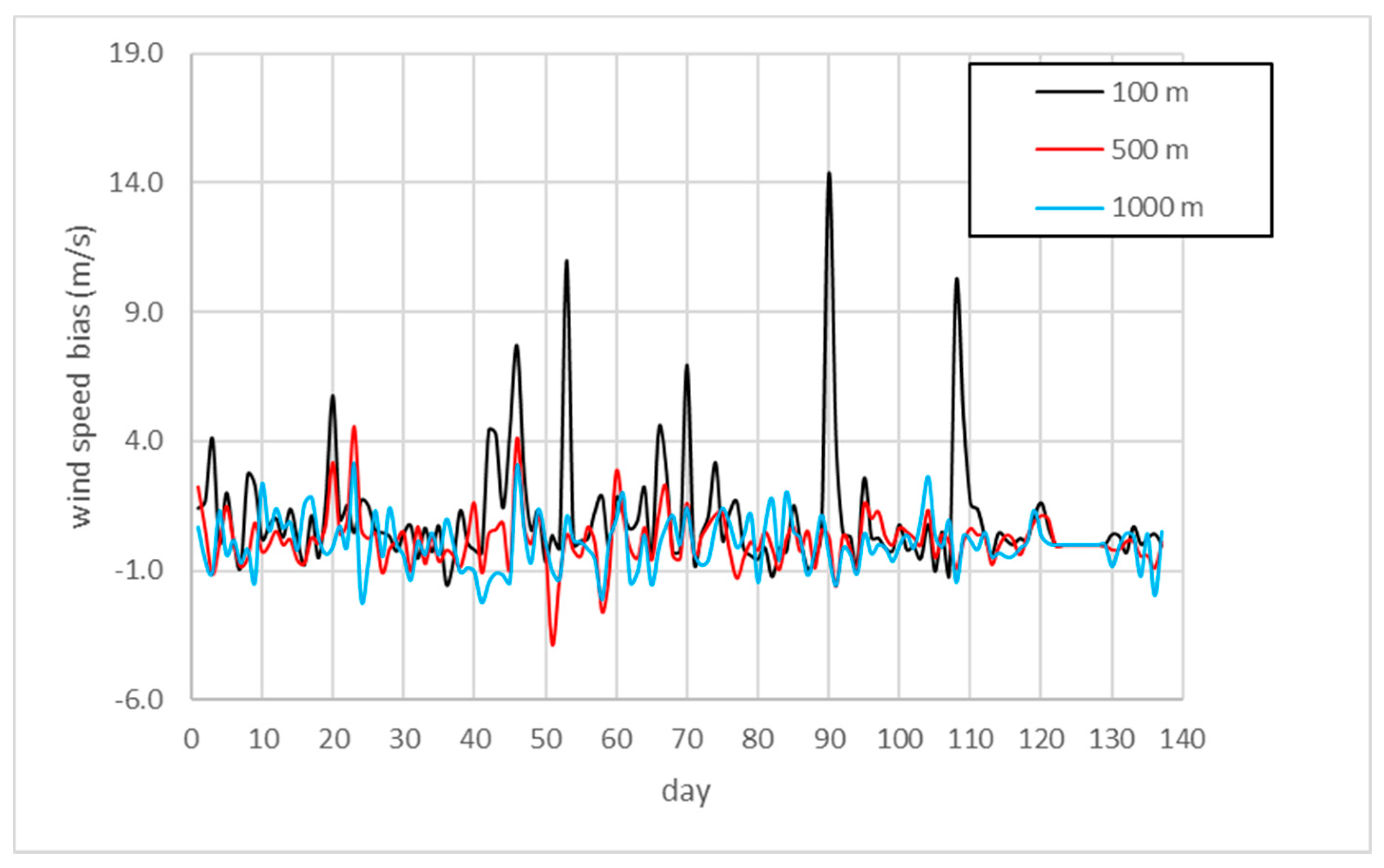
Figure 8 shows the daily bias values of wind speed at 100, 500 and 1000 m over the considered period, revealing the good capability of the model to reproduce daily values, especially at 500 and 1000 m. The bias generally was between −2 and +2 m/s and agreed with the results presented by Heppelmann et al. [
6]. Large biases recorded on some days were partially due to the non-negligible number of missing observed hourly values.
Table 4 shows the average, maximum and minimum values of BIAS for the three levels over the entire period. RMSE,
d, CORR and STD_RATIO were obtained by averaging hourly values over all the levels. Good agreement was found in terms of BIAS, but compensation effects were present, as revealed by the larger maximum and minimum values and by the RMSE. The correlation and STD_RATIO values are quite good.
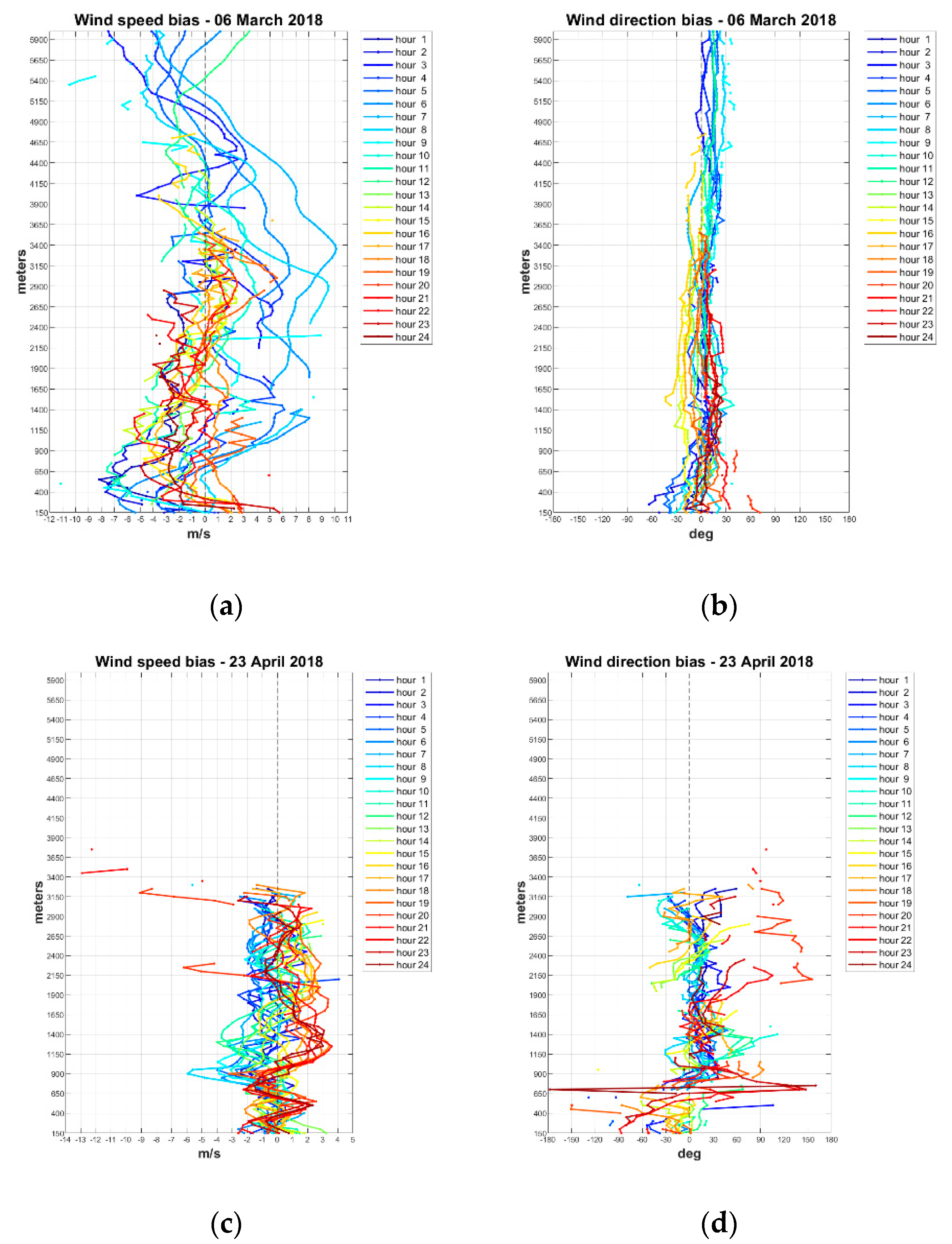
In order to investigate the origins of bias, vertical profiles were analyzed over selected days. As an example,
Figure 9 shows the vertical profiles of speed and direction bias on 6 March 2018 and 23 April 2018, the first one being a day with larger wind values and the second one with lower values. These figures contain the profiles for each hour of the day. Direction bias was evaluated only when the related speed was larger than 2 m/s. Part of the recorded bias was certainly due to the interpolation procedure required, since raw data are available at different geometrical heights, and also was due to the self-generated internal variability of the model simulation, as shown in [
36]. Moreover, the sharp reduction in wind speed at low altitudes, which is due to increased vertical mixing after sunrise, was simulated late by the COSMO model. Wind speed could potentially be enhanced by improving the PBL parameterization schemes [
23], and in particular regarding a source term for the prognostic turbulent kinetic energy and the description of the minimal diffusion coefficient [
6]. Both modifications will become operational in the ICON model [
37], which will improve the representation of stably stratified nights and the corresponding nocturnal wind speeds.
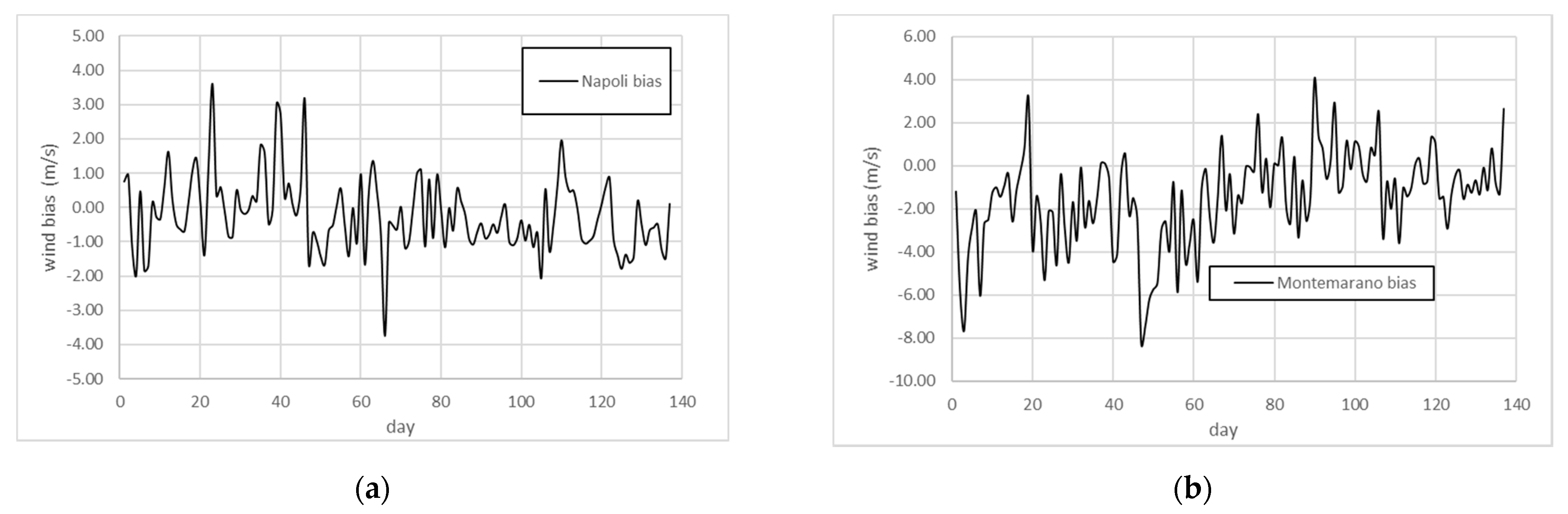
Next, model performance was investigated in Napoli Capodichino and Montemarano. For these locations, only ground station wind intensity values at 10 m were available.
Figure 10 shows daily bias values of wind speed over the considered period and confirms the good capabilities of the model in reproducing daily values at 10 m, in both locations, with bias generally between −2 and 2 m/s.
3.4. Radio Sounding Evaluation
Radio soundings are used to observe conventional upper-air conditions. Their high vertical resolution delivers good-quality observations and is a powerful benchmark for NWP evaluations. Unfortunately, the global distribution does not guarantee a uniform and detailed network, being confined to a limited number of locations. In the present work, data were provided by the radio sounding measured daily at the Pratica di Mare airport (at 00 and 12 UTC) and were compared with the values provided by COSMO in the grid point closest to this location.
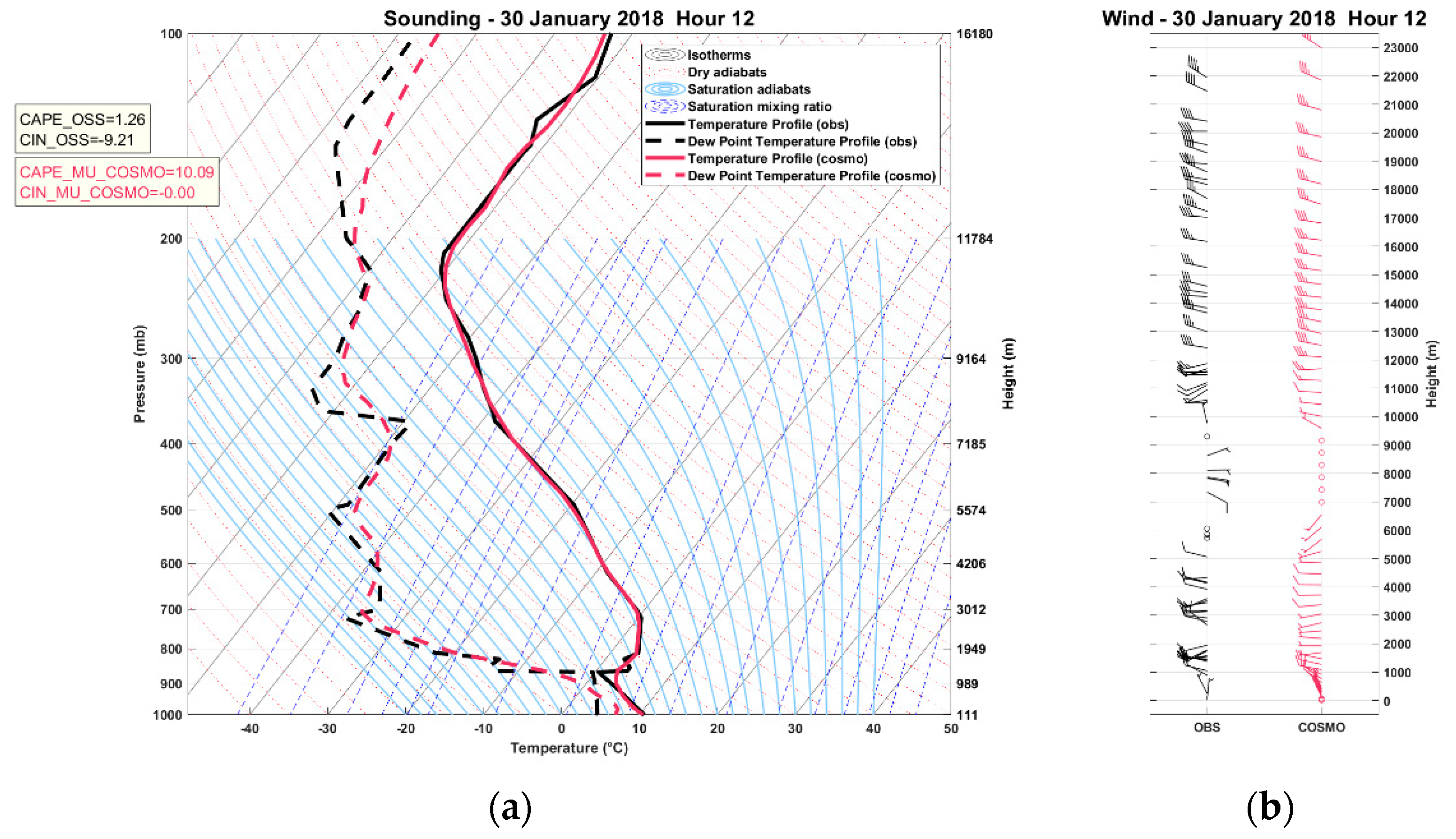
Table 5 shows the values (average, maximum and minimum) of BIAS, RMSE, CORR and STD_RATIO related to temperature, dew point, wind speed and direction, averaged over all the vertical values (up to 16 km altitude) and over all the days in the period considered. Results highlight a very good reproduction of the temperature profile (correlation equal to 1 and maximum bias of 1 °C) and also a good accuracy for the other variables. As an example,
Figure 11 shows the vertical profile of temperature and dew point (model and observations) on 30 January 2018 at 12 UTC. Wind barb vertical profiles are also shown. Part of the wind discrepancy can be due to some limitations in radiosonde measurements [
38], since radiosonde encounters a narrow column of air as it ascends, and a misleading profile may be produced if wind passes through the only cloud in the area. Moreover, the profile is not actually vertical due to the lateral drift of the balloon. Dew point temperature profiles are generally well reproduced, with the exception of the inversion points.
3.5. Evaluation against Ceilometer Data
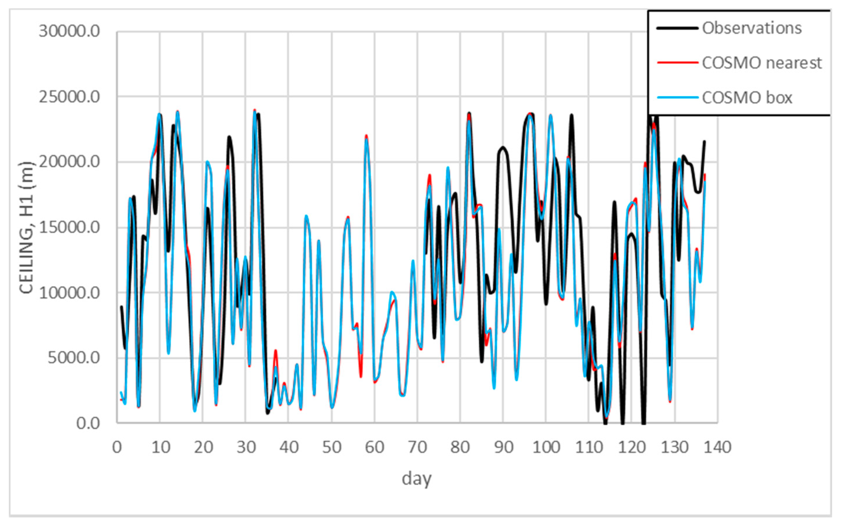
Ceilometer data were used to check the model’s capability to reproduce cloud heights. The COSMO output variable CEILING was considered, which indicates (in meters) the height above mean sea level at which cloud coverage is larger than 4/8.
Figure 12 shows the daily values of this variable (related to the nearest and 3 × 3 grid box) provided by the model and the height of the first cloud detected by the ceilometer (H1) (note that in the period 21 February–26 March 2018 observational data were not available). A general good agreement between the model and observations was recorded, with an average bias over the entire period of about +7.2%. However, non-negligible biases were recorded on some days: for example, on 6 May the model value was 4240 m while the observed value was 1170 m, demonstrating the existence of some deficiency in the treatment of surface–atmosphere interactions in the model [
39].
It is recognized that measuring the planetary boundary layer height (HPBL) is important not only for weather prediction, but also for air pollution analysis. Several studies have revealed the usefulness of ceilometers as a means to recognize and determine HPBL values [
40]. In particular, it is possible to calculate the mixing layer height (MLH) with specific algorithms [
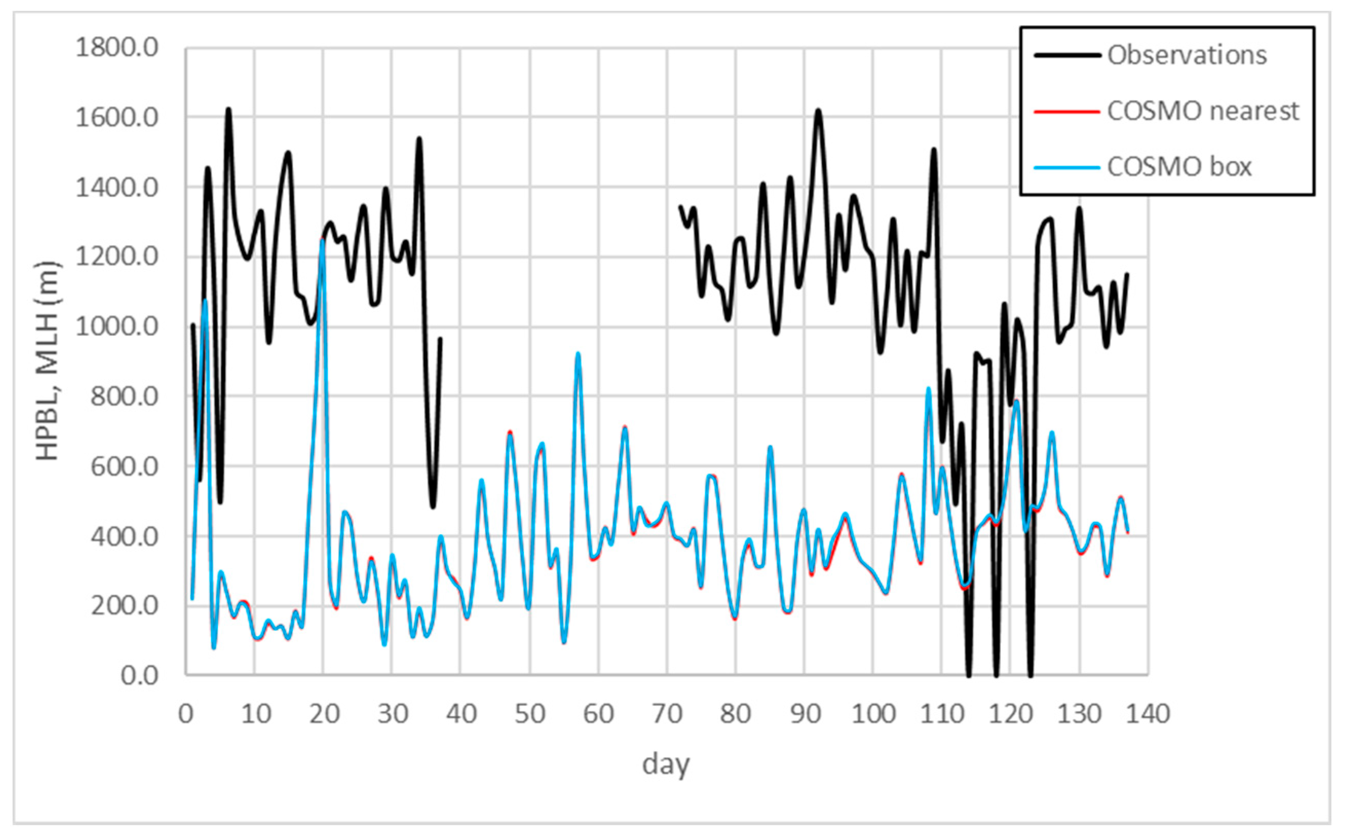
26] starting from the backscatter profiles provided by the instrument. In the present work, MLH values were used as a reference for validating the HPBL provided by the COSMO model, as MLH is a key parameter to characterize (with a certain degree of approximation) the structure of the PBL.
Figure 13 shows the daily values of HPBL (m) provided by the model, related to the nearest point and averaged over a 3 × 3 box, compared to MLH values for the whole period considered. It is evident that there were no differences between the nearest point and 3 × 3 box. In both cases, however, the trend seems to be qualitatively reproduced. COSMO largely underestimated the values of HPBL. Only in May 2018 when the weather was mild, with higher temperatures (see
Figure 2), was a better agreement observed. Part of this underestimation is certainly due to inaccuracies in the algorithm for MLH evaluation, as MLH detection could be adversely affected by the presence of clouds. These results highlight that tuning COSMO for HPBL evaluation is still a challenging research area. In any case, as stated also in [
7], the combination of high-resolution COSMO data and ceilometer data provides a correct evolution of PBL height.
4. Conclusions
In this paper, the results of simulations performed with the COSMO model at very high resolution over a domain located in southern Italy have been presented. The main aim of this work was to test the capabilities of the model by taking advantage of the wide range of technical instrumentation available at CIRA, which provides highly accurate observational data. A five-month period in winter/spring of 2018 was selected. In order to support different strategical sectors (e.g., flood, agriculture, renewable energy, tourism, civil protection), the NWP model output needs to be improved and optimized, but as a first step the forecast quality and model deficiencies must be understood. It is well known that a 1 km resolution is challenging to employ in weather models for short- and medium-term forecasts. Considering the computational costs required, it is necessary to evaluate if such simulations could provide good results, at least in complex orographic areas such as southern Italy.
The model was configured and optimized for the specific area of southern Italy, as in a previous work [
10] it was found that COSMO was highly sensitive to changes related to the physical soil and atmosphere parameters. In particular, it was shown that the present configuration adequately reduced temperature bias (up to 0.5 °C) and precipitation (even if benefits were less evident) over this complex orographic area. The distribution of vertical levels adopted by the model, both in the atmosphere and in the soil, provided better results compared to those by COSMO. Numerical tests on this topic were performed in [
41] with different resolutions and time horizons. Evidence of the model’s accuracy in simulating daily t2m is given by the low average biases, while nocturnal hourly values were underestimated. Regarding precipitation, dry days were generally well reproduced, while precipitation on rainy days was underestimated since COSMO experiences difficulties in localizing rain events in this complex orography area. Wind values were well reproduced, especially at high altitudes, suggesting a great potential of the model to support wind power production. Comparison with radio sounding data showed that the vertical profiles of temperature and dew point were well reproduced, with the exception of the inversion points. Finally, cloud height values were compared with those provided by the ceilometer, which showed good agreement, while preliminary results evaluating the planetary boundary layer height showed low accuracy. However, this offers a preview of the great potential of ceilometer data to evaluate mixing layer height.
Further improvements could be achieved by investigating other challenging areas, such as the use of urban parameterizations, which seem able to better reproduce key urban meteorological features [
32,
33] and the ensemble modelling approach. The area in the present study is characterized by a large number of buildings, and the area is close to the coast and orographically complex, so it is potentially more sensitive than others to the land surface processes. The urban canopy is a key issue not limited to the present test case; in fact, there are currently several studies in progress in the COSMO consortium that show the importance and the great sensitivity of the model to this issue. Several tests conducted in other areas (Turin, Moscow) (Garbero et al., paper submitted) have shown the relevant impacts of both the land surface scheme TERRA implemented in COSMO and of the urban parameterization scheme TERRA-URB on temperature (at least 0.5°). In particular, a new description of the surface temperature in TERRA is based on skin temperature formulations, which introduces an additional temperature of the canopy leaves (the skin temperature) as a way to represent energetically balanced vegetation on the surface [
33].
The present results represent a solid foundation for the implementation and testing of ICON [
37], the new model based on an icosahedral grid that will replace COSMO in the coming years. Similar analyses will be performed in the future to quantify the potential benefits provided by the new model.


