Carbon, Nitrogen, and Sulfur Elemental Fluxes in the Soil and Exchanges with the Atmosphere in Australian Tropical, Temperate, and Arid Wetlands


Abstract

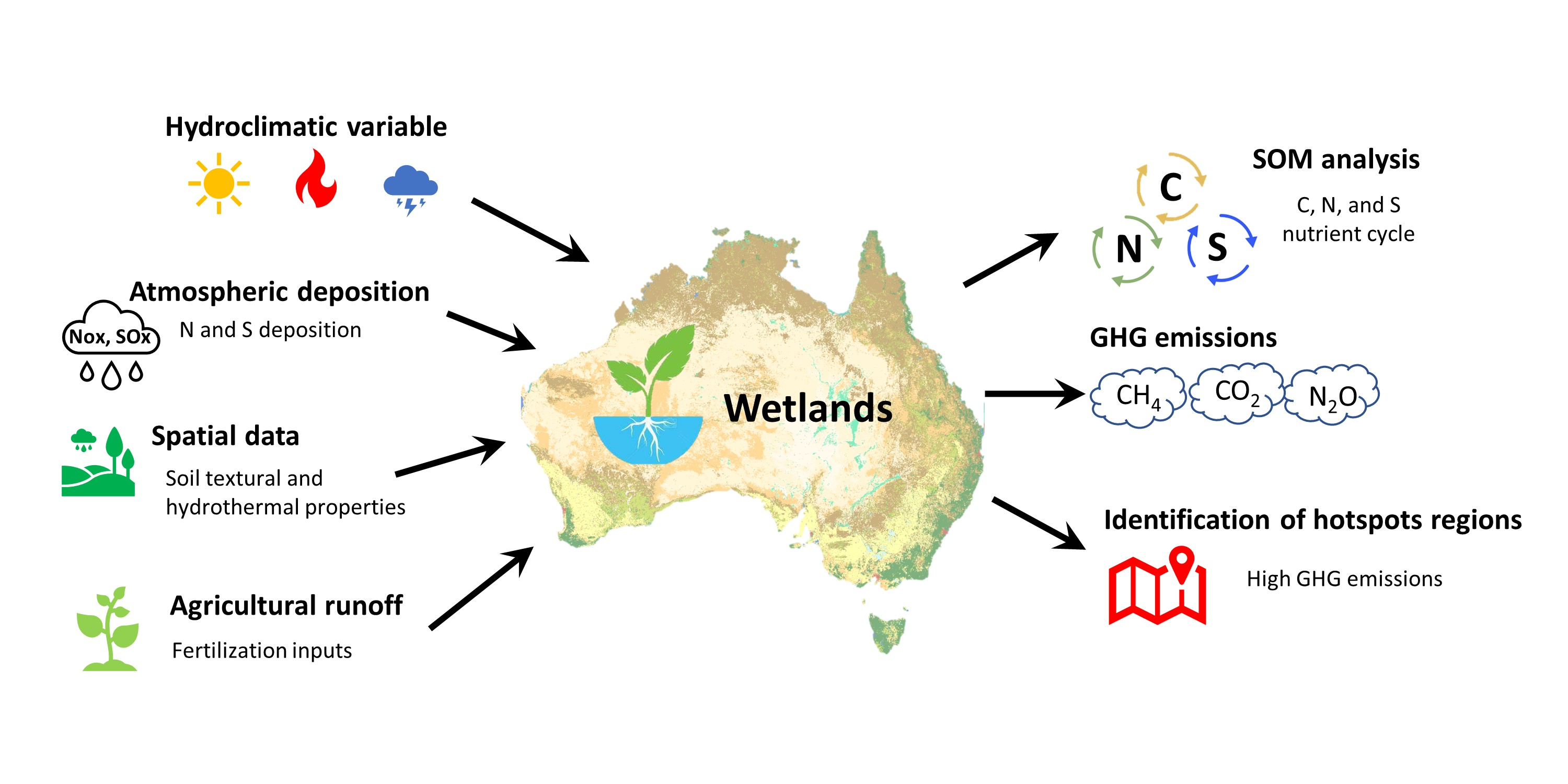
1. Introduction
2. Materials and Methods
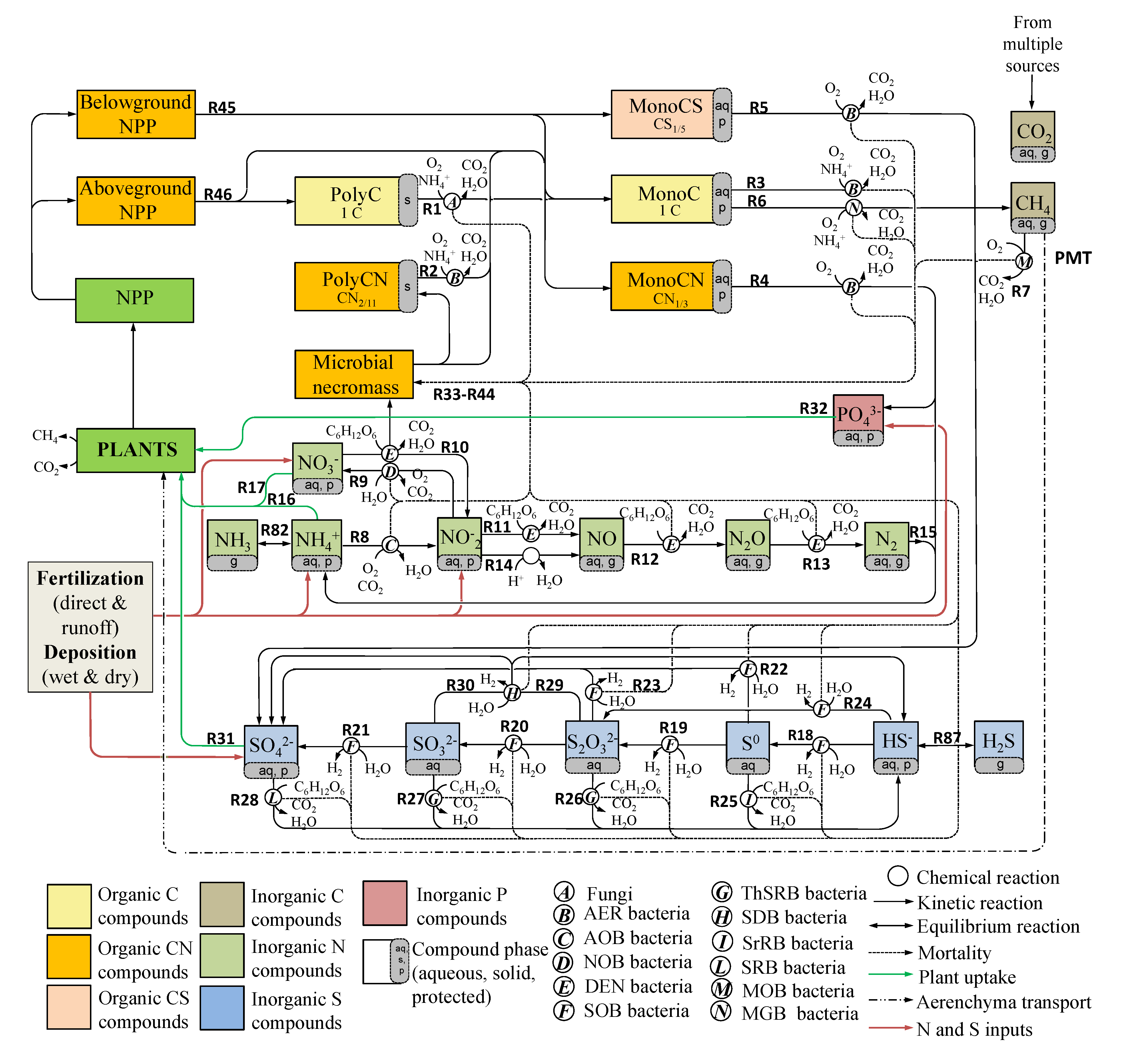
2.1. BAMS4 Biogeochemical Network
2.2. Dataset
2.3. Computational Domain and the BRTSim Solver
2.4. Methods of Analysis
3. Results
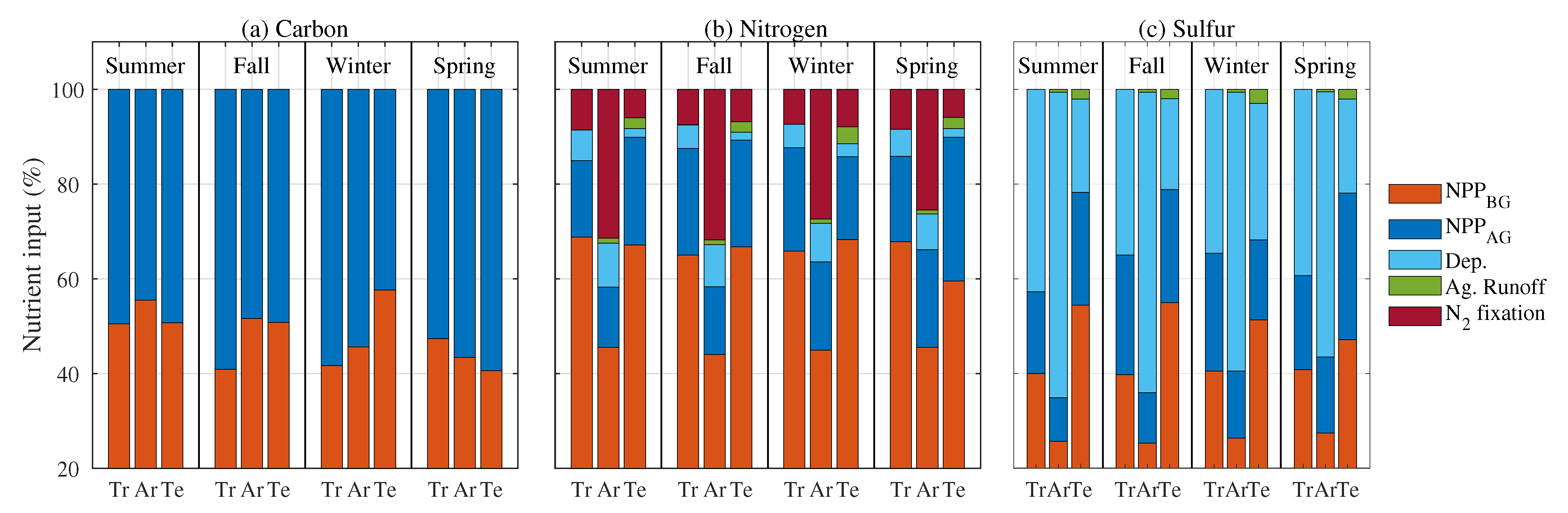
3.1. Inputs to Soil
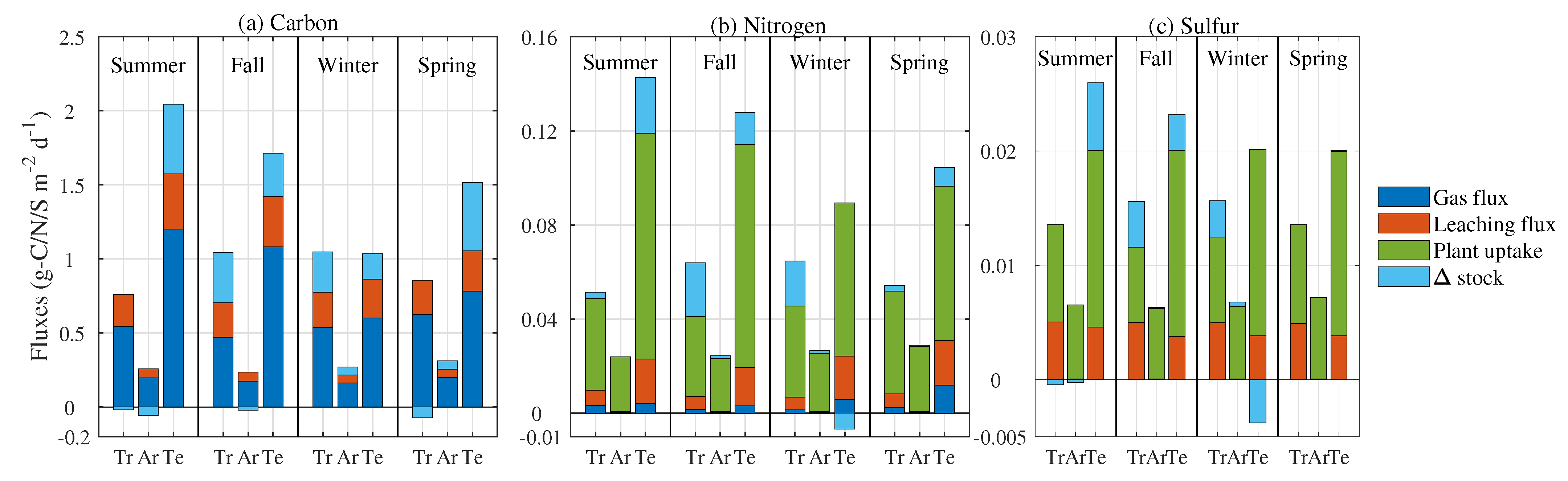
3.2. C, N, and S Fluxes in Soil
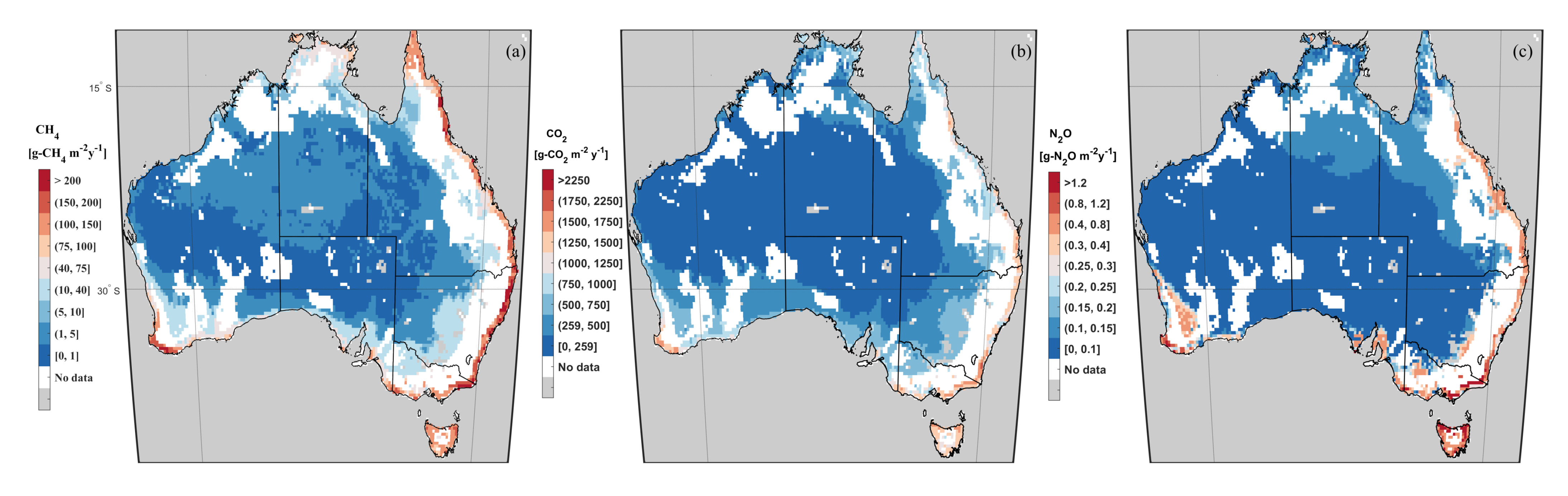
3.3. GHG Emissions
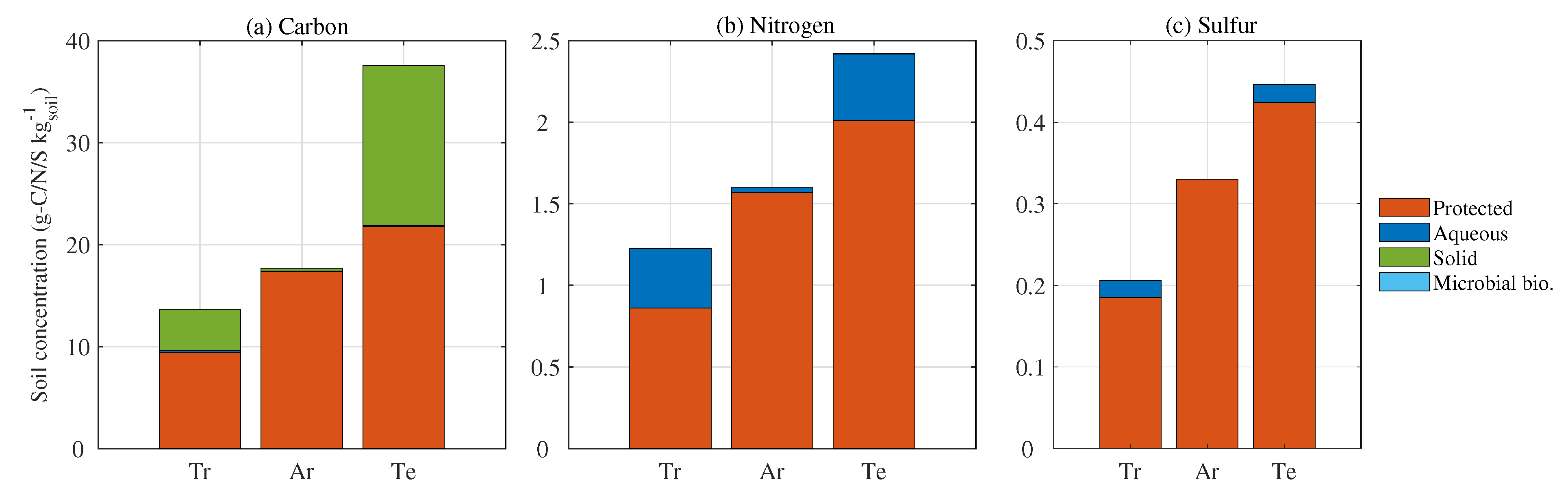
3.4. Phase Fractions in Soil
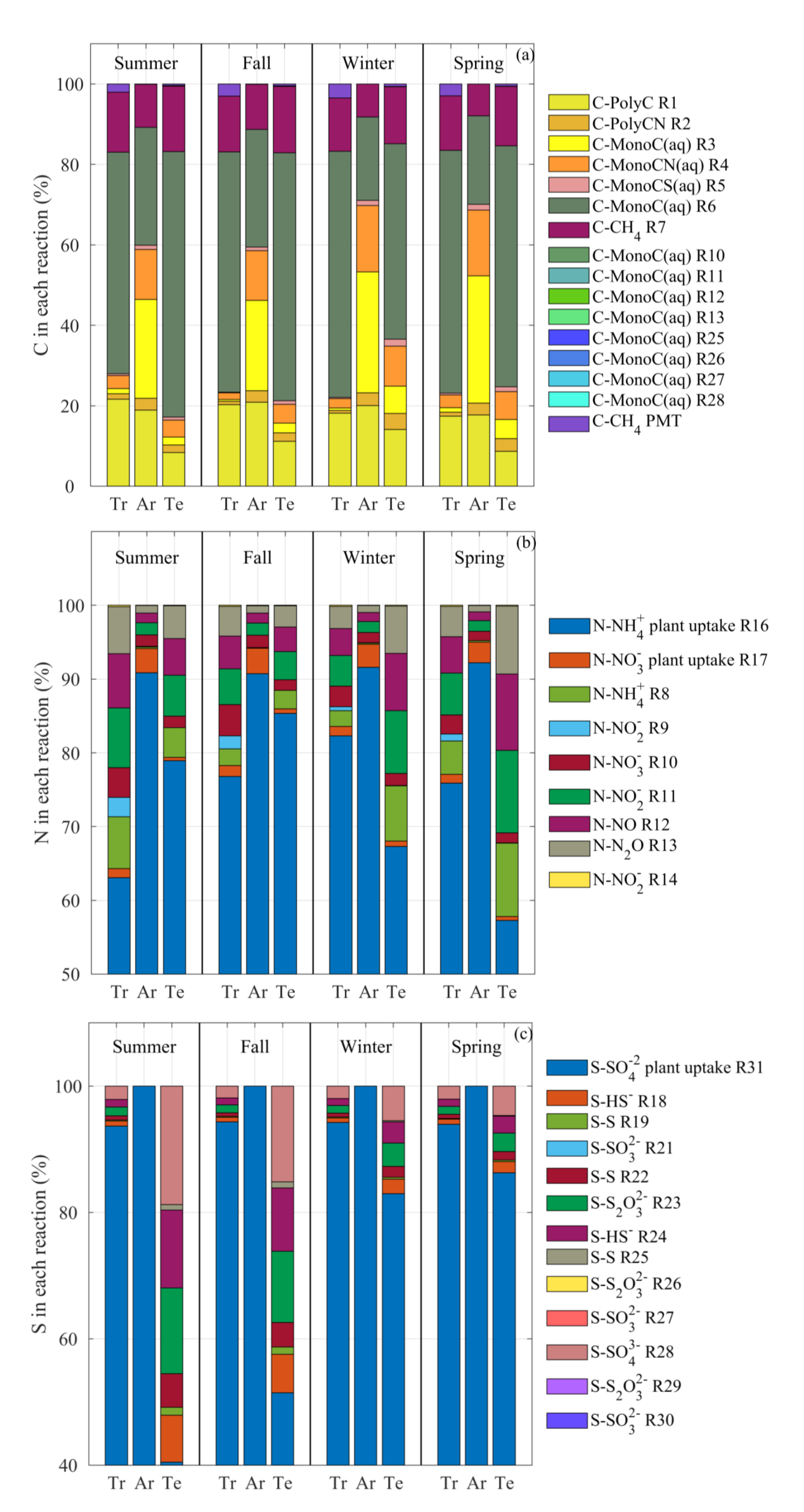
3.5. Mass Flux Partitioning
4. Discussion
5. Conclusions
Supplementary Materials
Author Contributions
Funding
Institutional Review Board Statement
Informed Consent Statement
Data Availability Statement
Acknowledgments
Conflicts of Interest
References
- Hensen, M.; Mahony, E. Reversing drivers of degradation in Blue Mountains and Newnes Plateau Shrub Swamp endangered ecological communities. Australas. Plant Conserv. J. Aust. Netw. Plant Conserv. 2010, 18, 5. [Google Scholar]
- Kohlhagen, T.; Fryirs, K.; Semple, A.L. Highlighting the Need and Potential for Use of Interdisciplinary Science in Adaptive Environmental Management: The Case of Endangered Upland Swamps in the B lue M ountains, NSW, A ustralia. Geogr. Res. 2013, 51, 439–453. [Google Scholar]
- Williams, A.A.; Stone, R.C. An assessment of relationships between the Australian subtropical ridge, rainfall variability, and high- latitude circulation patterns. Int. J. Climatol. J. R. Meteorol. Soc. 2009, 29, 691–709. [Google Scholar] [CrossRef]
- Morris, J.T.; Sundareshwar, P.; Nietch, C.T.; Kjerfve, B.; Cahoon, D.R. Responses of coastal wetlands to rising sea level. Ecology 2002, 83, 2869–2877. [Google Scholar] [CrossRef]
- Raabe, E.A.; Stumpf, R.P. Expansion of tidal marsh in response to sea-level rise: Gulf Coast of Florida, USA. Estuaries Coasts 2016, 39, 145–157. [Google Scholar] [CrossRef]
- Schuerch, M.; Spencer, T.; Temmerman, S.; Kirwan, M.L.; Wolff, C.; Lincke, D.; McOwen, C.J.; Pickering, M.D.; Reef, R.; Vafeidis, A.T.; et al. Future response of global coastal wetlands to sea-level rise. Nature 2018, 561, 231–234. [Google Scholar] [CrossRef]
- Krauss, K.W.; Noe, G.B.; Duberstein, J.A.; Conner, W.H.; Stagg, C.L.; Cormier, N.; Jones, M.C.; Bernhardt, C.E.; Graeme Lockaby, B.; From, A.S.; et al. The role of the upper tidal estuary in wetland blue carbon storage and flux. Glob. Biogeochem. Cycles 2018, 32, 817–839. [Google Scholar] [CrossRef]
- Baccini, A.; Walker, W.; Carvalho, L.; Farina, M.; Sulla-Menashe, D.; Houghton, R. Tropical forests are a net carbon source based on aboveground measurements of gain and loss. Science 2017, 358, 230–234. [Google Scholar] [CrossRef]
- Gourley, C.; Weaver, D. Nutrient surpluses in Australian grazing systems: Management practices, policy approaches, and difficult choices to improve water quality. Crop. Pasture Sci. 2013, 63, 805–818. [Google Scholar] [CrossRef]
- Rawnsley, R.; Smith, A.; Christie, K.; Harrison, M.; Eckard, R. Current and future direction of nitrogen fertiliser use in Australian grazing systems. Crop. Pasture Sci. 2020, 70, 1034–1043. [Google Scholar] [CrossRef]
- Gourley, C.J.; Dougherty, W.J.; Weaver, D.M.; Aarons, S.R.; Awty, I.M.; Gibson, D.M.; Hannah, M.C.; Smith, A.P.; Peverill, K.I. Farm-scale nitrogen, phosphorus, potassium and sulfur balances and use efficiencies on Australian dairy farms. Anim. Prod. Sci. 2012, 52, 929–944. [Google Scholar] [CrossRef]
- Eckard, R.; Chen, D.; White, R.; Chapman, D. Gaseous nitrogen loss from temperate perennial grass and clover dairy pastures in south-eastern Australia. Aust. J. Agric. Res. 2003, 54, 561–570. [Google Scholar] [CrossRef]
- De Klein, C.; Eckard, R. Targeted technologies for nitrous oxide abatement from animal agriculture. Aust. J. Exp. Agric. 2008, 48, 14–20. [Google Scholar] [CrossRef]
- IPCC. Synthesis Report. Contribution of Working Groups I, II and III to the Fifth Assessment Report of the Intergovernmental Panel on Climate Change-Intergovernmental Panel on Climate Change; IPCC: Geneva, Switzerland, 2014; p. 151. [Google Scholar]
- Middleton, B.A. Differences in impacts of Hurricane Sandy on freshwater swamps on the Delmarva Peninsula, Mid-Atlantic Coast, USA. Ecol. Eng. 2016, 87, 62–70. [Google Scholar] [CrossRef]
- Middleton, B.A. Effects of salinity and flooding on post-hurricane regeneration potential in coastal wetland vegetation. Am. J. Bot. 2016, 103, 1420–1435. [Google Scholar] [CrossRef] [PubMed]
- Kaushal, S.S.; Mayer, P.M.; Vidon, P.G.; Smith, R.M.; Pennino, M.J.; Newcomer, T.A.; Duan, S.; Welty, C.; Belt, K.T. Land use and climate variability amplify carbon, nutrient, and contaminant pulses: A review with management implications. JAWRA J. Am. Water Resour. Assoc. 2014, 50, 585–614. [Google Scholar] [CrossRef]
- Riley, W.; Subin, Z.; Lawrence, D.; Swenson, S.; Torn, M.; Meng, L.; Mahowald, N.; Hess, P. Barriers to predicting changes in global terrestrial methane fluxes: Analyses using CLM4Me, a methane biogeochemistry model integrated in CESM. Biogeosciences 2011, 8, 1925–1953. [Google Scholar] [CrossRef]
- Melton, J.; Wania, R.; Hodson, E.; Poulter, B.; Ringeval, B.; Spahni, R.; Bohn, T.; Avis, C.; Beerling, D.; Chen, G.; et al. Present state of global wetland extent and wetland methane modelling: Conclusions from a model inter-comparison project (WETCHIMP). Biogeosciences 2013, 10, 753–788. [Google Scholar] [CrossRef]
- Tian, H.; Chen, G.; Lu, C.; Xu, X.; Ren, W.; Zhang, B.; Banger, K.; Tao, B.; Pan, S.; Liu, M.; et al. Global methane and nitrous oxide emissions from terrestrial ecosystems due to multiple environmental changes. Ecosyst. Health Sustain. 2015, 1, 1–20. [Google Scholar] [CrossRef]
- Grant, R.; Mekonnen, Z.; Riley, W. Modeling climate change impacts on an Arctic polygonal tundra: 1. Rates of permafrost thaw depend on changes in vegetation and drainage. J. Geophys. Res. Biogeosci. 2019, 124, 1308–1322. [Google Scholar] [CrossRef]
- Chang, K.Y.; Riley, W.J.; Brodie, E.L.; McCalley, C.K.; Crill, P.M.; Grant, R.F. Methane Production Pathway Regulated Proximally by Substrate Availability and Distally by Temperature in a High-Latitude Mire Complex. J. Geophys. Res. Biogeosci. 2019, 124, 3057–3074. [Google Scholar] [CrossRef]
- Beerling, D.J.; Fox, A.; Stevenson, D.S.; Valdes, P.J. Enhanced chemistry-climate feedbacks in past greenhouse worlds. Proc. Natl. Acad. Sci. USA 2011, 108, 9770–9775. [Google Scholar] [CrossRef] [PubMed]
- Wania, R.; Melton, J.; Hodson, E.L.; Poulter, B.; Ringeval, B.; Spahni, R.; Bohn, T.; Avis, C.; Chen, G.; Eliseev, A.V.; et al. Present state of global wetland extent and wetland methane modelling: Methodology of a model inter-comparison project (WETCHIMP). Geosci. Model Dev. 2013, 6, 617–641. [Google Scholar] [CrossRef]
- Pasut, C.; Tang, F.H.; Maggi, F. A Mechanistic Analysis of Wetland Biogeochemistry in Response to Temperature, Vegetation, and Nutrient Input Changes. J. Geophys. Res. Biogeosci. 2020, 125, e2019JG005437. [Google Scholar] [CrossRef]
- Riley, W.; Maggi, F.; Kleber, M.; Torn, M.; Tang, J.; Dwivedi, D.; Guerry, N. Long residence times of rapidly decomposable soil organic matter: Application of a multi-phase, multi-component, and vertically resolved model (BAMS1) to soil carbon dynamics. Geosci. Model Dev. 2014, 7, 1335–1355. [Google Scholar] [CrossRef]
- Tang, F.H.; Riley, W.J.; Maggi, F. Hourly and daily rainfall intensification causes opposing effects on C and N emissions, storage, and leaching in dry and wet grasslands. Biogeochemistry 2019, 144, 197–214. [Google Scholar] [CrossRef]
- Ceriotti, G.; Tang, F.; Maggi, F. Similarities and differences in the sensitivity of soil organic matter (SOM) dynamics to biogeochemical parameters for different vegetation inputs and climates. Stoch. Environ. Res. Risk Assess. 2020, 34, 2229–2244. [Google Scholar] [CrossRef]
- Schroeder, R.; McDonald, K.C.; Chapman, B.D.; Jensen, K.; Podest, E.; Tessler, Z.D.; Bohn, T.J.; Zimmermann, R. Development and evaluation of a multi-year fractional surface water data set derived from active/passive microwave remote sensing data. Remote. Sens. 2015, 7, 16688–16732. [Google Scholar] [CrossRef]
- Poulter, B.; Bousquet, P.; Canadell, J.G.; Ciais, P.; Peregon, A.; Saunois, M.; Arora, V.K.; Beerling, D.J.; Brovkin, V.; Jones, C.D.; et al. Global wetland contribution to 2000–2012 atmospheric methane growth rate dynamics. Environ. Res. Lett. 2017, 12, 094013. [Google Scholar] [CrossRef]
- Zhang, Y.; Pena Arancibia, J.; McVicar, T.; Chiew, F.; Vaze, J.; Zheng, H.; Wang, Y. Monthly Global Observation-Driven Penman–Monteith–Leuning (Pml) Evapotranspiration and Components. 2016. Available online: https://data.csiro.au/dap/landingpage?pid=csiro%3A17375 (accessed on 1 November 2020).
- Yukimoto, S.; Koshiro, T.; Kawai, H.; Oshima, N.; Yoshida, K.; Urakawa, S.; Tsujino, H.; Deushi, M.; Tanaka, T.; Hosaka, M.; et al. Mri Mri-Esm2.0 Model Output Prepared for Cmip6 Cmip Historical. Available online: https://cera-www.dkrz.de/WDCC/ui/cerasearch/cmip6?input=CMIP6.CMIP.MRI.MRI-ESM2-0.historical (accessed on 1 November 2020).
- Hengl, T.; de Jesus, J.M.; Heuvelink, G.B.; Gonzalez, M.R.; Kilibarda, M.; Blagotić, A.; Shangguan, W.; Wright, M.N.; Geng, X.; Bauer-Marschallinger, B.; et al. SoilGrids250m: Global gridded soil information based on machine learning. PLoS ONE 2017, 12, e0169748. [Google Scholar] [CrossRef]
- Dai, Y.; Shangguan, W.; Duan, Q.; Liu, B.; Fu, S.; Niu, G. Development of a China dataset of soil hydraulic parameters using pedotransfer functions for land surface modeling. J. Hydrometeorol. 2013, 14, 869–887. [Google Scholar] [CrossRef]
- Potter, P.; Ramankutty, N.; Bennett, E.; Donner, S. Global fertilizer and manure, version 1: Nitrogen fertilizer application. Palisades NY Nasa Socioecon. Data Appl. Cent. (SEDAC) 2011, 10, H4FQ9TJR. [Google Scholar]
- Potter, P.; Ramankutty, N.; Bennett, E.; Donner, S. Global fertilizer and manure, version 1: Phosphorus fertilizer application. Palisades NY Nasa Socioecon. Data Appl. Cent. (SEDAC) 2011, 10, H4FQ9TJR. [Google Scholar]
- Canadell, J.; Jackson, R.; Ehleringer, J.; Mooney, H.; Sala, O.; Schulze, E.D. Maximum rooting depth of vegetation types at the global scale. Oecologia 1996, 108, 583–595. [Google Scholar] [CrossRef] [PubMed]
- Paul, E.A. Soil Microbiology, Ecology and Biochemistry; Academic Press: Burlington, USA, 2014. [Google Scholar]
- Walter, B.P.; Heimann, M.; Matthews, E. Modeling modern methane emissions from natural wetlands: 1. Model description and results. J. Geophys. Res. Atmos. 2001, 106, 34189–34206. [Google Scholar] [CrossRef]
- Rouifed, S.; Handa, I.T.; David, J.F.; Hättenschwiler, S. The importance of biotic factors in predicting global change effects on decomposition of temperate forest leaf litter. Oecologia 2010, 163, 247–256. [Google Scholar] [CrossRef] [PubMed]
- Hättenschwiler, S.; Jørgensen, H.B. Carbon quality rather than stoichiometry controls litter decomposition in a tropical rain forest. J. Ecol. 2010, 98, 754–763. [Google Scholar] [CrossRef]
- Pei, G.; Liu, J.; Peng, B.; Gao, D.; Wang, C.; Dai, W.; Jiang, P.; Bai, E. Nitrogen, lignin, C/N as important regulators of gross nitrogen release and immobilization during litter decomposition in a temperate forest ecosystem. For. Ecol. Manag. 2019, 440, 61–69. [Google Scholar] [CrossRef]
- Bréchet, L.; Le Dantec, V.; Ponton, S.; Goret, J.Y.; Sayer, E.; Bonal, D.; Freycon, V.; Roy, J.; Epron, D. Short-and long-term influence of litter quality and quantity on simulated heterotrophic soil respiration in a lowland tropical forest. Ecosystems 2017, 20, 1190–1204. [Google Scholar] [CrossRef]
- Snowdon, P.; Ryan, P.; Raison, R.J. Review of C:N Ratios In Vegetation, Litter and Soil under Australian Native Forests and Plantations; Australian Greenhouse Office: Canberra, Australian, 2005. [Google Scholar]
- Cover, M.L.; Change, L.C. Modis Land Cover Product Algorithm Theoretical Basis Document (Atbd) Version 5.0; MODIS documentation; University of Maryland: College Park, MD, USA, 1999; Volume 23, pp. 42–47. [Google Scholar]
- Hong, Y.; Adler, R. Estimation of global SCS curve numbers using satellite remote sensing and geospatial data. Int. J. Remote. Sens. 2008, 29, 471–477. [Google Scholar] [CrossRef]
- Lehner, B.; Döll, P. Development and validation of a global database of lakes, reservoirs and wetlands. J. Hydrol. 2004, 296, 1–22. [Google Scholar] [CrossRef]
- Köppen, W.; Geiger, G. Handbuch der Klimatologie-Gebrüder Borntraeger; Gerbrüder Bornträger: Berlin, Germany, 1936; pp. 1–44. [Google Scholar]
- Chang, K.Y.; Riley, W.J.; Crill, P.M.; Grant, R.F.; Saleska, S.R. Hysteretic temperature sensitivity of wetland CH 4 fluxes explained by substrate availability and microbial activity. Biogeosci. Discuss. 2020, 17, 1–38. [Google Scholar]
- Rohli, R.V.; Joyner, T.A.; Reynolds, S.J.; Ballinger, T.J. Overlap of global Köppen–Geiger climates, biomes, and soil orders. Phys. Geogr. 2015, 36, 158–175. [Google Scholar] [CrossRef]
- Saunois, M.; Stavert, A.R.; Poulter, B.; Bousquet, P.; Canadell, J.G.; Jackson, R.B.; Raymond, P.A.; Dlugokencky, E.J.; Houweling, S.; Patra, P.K.; et al. The global methane budget 2000–2017. Earth Syst. Sci. Data 2020, 12, 1561–1623. [Google Scholar] [CrossRef]
- Dalal, R.; Allen, D.; Livesley, S.; Richards, G. Magnitude and biophysical regulators of methane emission and consumption in the Australian agricultural, forest, and submerged landscapes: A review. Plant Soil 2008, 309, 43–76. [Google Scholar] [CrossRef]
- Bartlett, K.B.; Harriss, R.C. Review and assessment of methane emissions from wetlands. Chemosphere 1993, 26, 261–320. [Google Scholar] [CrossRef]
- Boon, P.; Lee, K. Methane oxidation in sediments of a floodplain wetland in south-eastern Australia. Lett. Appl. Microbiol. 1997, 25, 138–142. [Google Scholar] [CrossRef]
- Allen, D.E.; Dalal, R.C.; Rennenberg, H.; Meyer, R.L.; Reeves, S.; Schmidt, S. Spatial and temporal variation of nitrous oxide and methane flux between subtropical mangrove sediments and the atmosphere. Soil Biol. Biochem. 2007, 39, 622–631. [Google Scholar] [CrossRef]
- Devol, A.H.; Richey, J.E.; Forsberg, B.R.; Martinelli, L.A. Seasonal dynamics in methane emissions from the Amazon River floodplain to the troposphere. J. Geophys. Res. Atmos. 1990, 95, 16417–16426. [Google Scholar] [CrossRef]
- Kreuzwieser, J.; Buchholz, J.; Rennenberg, H. Emission of methane and nitrous oxide by Australian mangrove ecosystems. Plant Biol. 2003, 5, 423–431. [Google Scholar] [CrossRef]
- Menne, M.J.; Durre, I.; Vose, R.S.; Gleason, B.E.; Houston, T.G. An overview of the global historical climatology network-daily database. J. Atmos. Ocean. Technol. 2012, 29, 897–910. [Google Scholar] [CrossRef]
- Dunfield, P.; Dumont, R.; Moore, T.R. Methane production and consumption in temperate and subarctic peat soils: Response to temperature and pH. Soil Biol. Biochem. 1993, 25, 321–326. [Google Scholar] [CrossRef]
- Inglett, K.; Inglett, P.; Reddy, K.; Osborne, T. Temperature sensitivity of greenhouse gas production in wetland soils of different vegetation. Biogeochemistry 2012, 108, 77–90. [Google Scholar] [CrossRef]
- Cookson, W.R.; Abaye, D.A.; Marschner, P.; Murphy, D.V.; Stockdale, E.A.; Goulding, K.W. The contribution of soil organic matter fractions to carbon and nitrogen mineralization and microbial community size and structure. Soil Biol. Biochem. 2005, 37, 1726–1737. [Google Scholar] [CrossRef]
- Boughton, E.H.; Quintana-Ascencio, P.F.; Bohlen, P.J.; Nickerson, D. Differential facilitative and competitive effects of a dominant macrophyte in grazed subtropical wetlands. J. Ecol. 2011, 99, 1263–1271. [Google Scholar] [CrossRef]
- Knapp, A.K.; Fay, P.A.; Blair, J.M.; Collins, S.L.; Smith, M.D.; Carlisle, J.D.; Harper, C.W.; Danner, B.T.; Lett, M.S.; McCarron, J.K. Rainfall variability, carbon cycling, and plant species diversity in a mesic grassland. Science 2002, 298, 2202–2205. [Google Scholar] [CrossRef]
- Chou, W.W.; Silver, W.L.; Jackson, R.D.; Thompson, A.W.; Allen-Diaz, B. The sensitivity of annual grassland carbon cycling to the quantity and timing of rainfall. Glob. Chang. Biol. 2008, 14, 1382–1394. [Google Scholar] [CrossRef]
- Whiting, G.J.; Chanton, J. Primary production control of methane emission from wetlands. Nature 1993, 364, 794–795. [Google Scholar] [CrossRef]
- Hughes, L. Climate change and Australia: Trends, projections and impacts. Austral Ecol. 2003, 28, 423–443. [Google Scholar] [CrossRef]


| KG Class | C:N of Soil Input (g-C g-N) | C:S of Soil Input (g-C g-S) | ||||||||
|---|---|---|---|---|---|---|---|---|---|---|
| Summer | Fall | Winter | Spring | Average | Summer | Fall | Winter | Spring | Average | |
| Tropical | 14.04 | 16.37 | 16.28 | 14.74 | 15.35 | 54.71 | 67.13 | 67.10 | 59.41 | 62.09 |
| Arid | 8.44 | 8.77 | 10.14 | 10.80 | 9.53 | 31.88 | 33.84 | 39.90 | 43.63 | 37.31 |
| Temperate | 13.64 | 13.53 | 12.19 | 15.09 | 13.61 | 74.13 | 74.65 | 61.41 | 80.10 | 72.57 |
| C:N in the Root Zone (g-C g-N) | C:S in the Root Zone (g-C g-S) | |||||||||
| Tropical | 13.01 | 13.00 | 13.02 | 13.03 | 13.07 | 80.02 | 80.35 | 80.10 | 79.75 | 80.06 |
| Arid | 10.76 | 10.76 | 10.76 | 10.76 | 10.76 | 46.94 | 46.93 | 46.93 | 46.96 | 46.94 |
| Temperate | 18.69 | 18.68 | 18.70 | 18.71 | 18.70 | 18.70 | 98.43 | 98.42 | 98.27 | 98.35 |
| State/Territory | CH | CO | NO | Area |
|---|---|---|---|---|
| (Tg-CH y) | (Tg-CO y) | (Tg-NO y) | (10 km) | |
| New South Wales | 0.91 | 11.87 | 2.76 × 10 | 0.0231 |
| Victoria | 0.36 | 4.05 | 1.87 × 10 | 0.0053 |
| South Australia | 0.37 | 14.20 | 1.90 × 10 | 0.0738 |
| Western Australia | 0.72 | 22.00 | 3.15 × 10 | 0.1042 |
| Queensland | 1.57 | 20.50 | 6.40 × 10 | 0.0655 |
| Northern Territory | 0.80 | 14.08 | 4.42 × 10 | 0.0579 |
| Tasmania | 0.38 | 4.19 | 2.95 × 10 | 0.0037 |
| Australia | 5.12 | 90.89 | 2.34 × 10 | 0.3335 |
| Tropical | 1.53 | 15.08 | 3.58 × 10 | 0.0363 |
| Arid | 0.61 | 46.61 | 6.77 × 10 | 0.2640 |
| Temperate | 2.97 | 29.21 | 1.31 × 10 | 0.0333 |
Publisher’s Note: MDPI stays neutral with regard to jurisdictional claims in published maps and institutional affiliations. |
© 2020 by the authors. Licensee MDPI, Basel, Switzerland. This article is an open access article distributed under the terms and conditions of the Creative Commons Attribution (CC BY) license (http://creativecommons.org/licenses/by/4.0/).
Share and Cite
Pasut, C.; Tang, F.H.M.; Hamilton, D.P.; Maggi, F. Carbon, Nitrogen, and Sulfur Elemental Fluxes in the Soil and Exchanges with the Atmosphere in Australian Tropical, Temperate, and Arid Wetlands. Atmosphere 2021, 12, 42. https://doi.org/10.3390/atmos12010042
Pasut C, Tang FHM, Hamilton DP, Maggi F. Carbon, Nitrogen, and Sulfur Elemental Fluxes in the Soil and Exchanges with the Atmosphere in Australian Tropical, Temperate, and Arid Wetlands. Atmosphere. 2021; 12(1):42. https://doi.org/10.3390/atmos12010042
Chicago/Turabian StylePasut, Chiara, Fiona H. M. Tang, David P. Hamilton, and Federico Maggi. 2021. "Carbon, Nitrogen, and Sulfur Elemental Fluxes in the Soil and Exchanges with the Atmosphere in Australian Tropical, Temperate, and Arid Wetlands" Atmosphere 12, no. 1: 42. https://doi.org/10.3390/atmos12010042
APA StylePasut, C., Tang, F. H. M., Hamilton, D. P., & Maggi, F. (2021). Carbon, Nitrogen, and Sulfur Elemental Fluxes in the Soil and Exchanges with the Atmosphere in Australian Tropical, Temperate, and Arid Wetlands. Atmosphere, 12(1), 42. https://doi.org/10.3390/atmos12010042