Abstract
Annual cycle is fundamental in the East Asian monsoon (EAM) systems, profoundly governing the spatiotemporal distribution of the East Asian rainfall. The present study identified the dominant modes of the annual cycle in the East Asian rainfall based on the Fourier harmonic analysis and the Empirical Orthogonal Function (EOF) decomposition. We evaluated the performance of the first two leading modes (i.e., EOF-1 and EOF-2) in historical experiments (1979–2014) of the 21 released climate models of phase six of the Coupled Model Intercomparison Project (CMIP6). Comparing with the observation, although the CMIP6 models yield the essential fidelity, they still show considerable systematic biases in the amplitude and phase of the annual cycle, especially in east and south China. Most models exhibit substantial phase delays in the EOF-2 mode of the annual cycle. Some specific models (BCC-ESM1, CanESM5, and GFDL-CM4) exhibiting better performance could capture the observed annual cycle and the underlying physics in climatology and interannual variability. The limited fidelity of the EOF-2 mode of the EAM annual cycle primarily hinders the monsoon variability simulation and thus the reliable future projection. Therefore, the dominant modes of the EAM annual cycle act as the evaluate benchmark in the EAM modelling framework. Their improvement could be one possible bias correction strategy for decreasing the uncertainty in the CMIP6 simulation of the EAM.
1. Introduction
Asian monsoon precipitation feeds billions of people over the regions with the world’s most dense population [1]. There is an urgent demand to address food security and agricultural practices caused by precipitation-related severe disasters, such as anomalous floods and droughts. Hence, precipitation is an essential factor in predicting climate variabilities given its tremendous impact on public health, socioeconomic risk, and ecological balance. However, Asian monsoon rainfall, characterized by the multiple spatiotemporal scales and multi-scale interactions, is still challenging to predict. Despite its extremely heterogeneous structure and diverse behavior, the remarkable annual cycle of the Asian monsoon depends on the large-scale underlying forcing and constraints, which provides higher predictability than the monsoon rainfall in a given period. The global monsoon, as a global-scale solstitial mode featuring the seasonal variation of monsoon precipitation, is forced by the annual cycle of solar radiation [2,3,4,5]. In particular, the subtropical East Asian (EA) and tropical western North Pacific (WNP) monsoonal circulations are driven by the solar radiation [6] and regulated by the sharp land–sea thermal contrast [6,7,8] and complex terrain (i.e., topographic uplift of the Tibet Plateau and various surrounding mountain chains [9,10,11,12,13]), among others.
Rainfall in the East Asia-western North Pacific (EA-WNP) region exhibits a distinctive and remarkable annual cycle. Traditionally, the rainfall distribution includes five rainy periods associated with the annual cycle over the EA-WNP domain [14,15,16,17]. The abrupt change in monsoonal circulation over southeastern Asia accompanies the first rainy peak of the Meiyu/Baiu rainfall in early–mid-summer [18,19]. The northward jump of the convection in WNP follows the second peak of the WNP typhoon rainfall in deep summer [6,20,21]. In the dry winter period, the continental Siberian high and large-scale northerly winter monsoon winds anchor the main rainband to the east of Japan. Two transition periods between them are the tilting spring rainband and fall frontal rainfall, respectively. They are affected by different atmospheric and oceanic conditions [16,22,23,24,25]. Conspicuously, the summer rainbands over the East Asian continent are associated with different steps of the monsoon cycle. They present the northward migration of the primary narrow rain belt from the south (pre-monsoon rain) to central (Meiyu/Baiu front) and to North China (the polar front) [26,27,28].
Due to the uniqueness and complexity of the annual cycle over EA, general circulation models (GCMs) have long struggled with numerous challenges in reproducing the realistic rainfall distribution and rain belt structure [29,30,31,32,33]. The GCMs possess considerable biases in simulating the location and seasonal evolution of East Asian rainfall [34,35,36]. In boreal summer, the GCMs generally underestimated the intensity of summer monsoon and rainfall over East Asia [29,37,38,39]. In contrast, multi-model ensembles overestimate the tropical rainfall of the WNP summer monsoon (WNPSM) [29,32]. Lambert and Boer [40] indicated that rainfall biases were significant over the Asian summer monsoon (ASM) domain by comparing the CMIP1 results to the observation. In recent decades, CMIP3 and CMIP5 models face the same predicament and have slight improvements partly due to the higher-resolution and subgrid-scale parameterization [29,38,41]. Additionally, other rainy periods also exhibit distinct biases and great diversity among the climate models [42,43,44,45,46].
Large biases with non-uniformed distribution prevail in all seasons. The GCMs are hard to mimic the monsoon northward migration and the seasonal propagation of the rainband in observation [36,37,47,48,49]. For instance, the AMIP1 models showed a large bias in simulating the annual cycle of eastern China monsoon rainfall [30]. Afterward, the CMIP3 ensembles cannot sufficiently capture the observed northward movement of the East Asian rainband, although they exhibit a developing inter-model consensus on the timing of the rainy season [34].
Understanding the rainfall distribution all year round is vital for timely water management, natural disaster prevention, and power generation. By now, the variation of the seasonal-mean rainfall has attracted more attention when considering the GCMs performances, but we commonly dismissed the dry seasons and transition seasons. Better simulation of the annual cycle of the EA rainfall increases the seasonal prediction accuracy and decreases the uncertainty of the future projection. Due to the improved parameterizations and higher resolutions, incremental improvements were achieved from CMIP3 to CMIP5 and CMIP6 [50]. The CMIP6 models can better simulate the monsoon precipitation comparing with the CMIP5 models [51,52,53]. Thereby, we can expect that the CMIP6 models can reasonably reproduce the EA-WNP monsoon cycle. This study aims to objectively evaluate the CMIP6 performance of the annual cycle of EA rainfall.
The remainder of the paper is organized as follows. Section 2 introduces the datasets from the CMIP6 archive and observations, and methods. The simulation deficiencies of the primary spatio-temporal structures of the East Asian annual cycle are demonstrated in Section 3. Section 4 focuses on the EOF modes of the annual cycle and proposes a new benchmark to evaluate the model performances. Section 5 is the major conclusions and discussion.
2. Data and Methods
2.1. CMIP6 Archive and Observation
In this study, the main focus is on the most recent state-of-the-art simulations from the CMIP6 GCMs and Earth system models (ESMs) [50]. We analyze daily precipitation, horizontal wind, sea level pressure (SLP) for the historical period (extending from 1850 to 2014, all-forcing experiment, hereafter HIST) of 21 released CMIP6 models (Table 1). Only one ensemble member for each model has been used and occupied equal weightage when calculating the multi-model ensemble (MME) mean. Given the various spatial resolutions of CMIP6 models, we first interpolated all participating model outputs into a regular grid of 2.5° × 2.5° using the bilinear interpolation methods. The period from 1979 to 2014 is adopted as the baseline of the climatology. The pentad-mean records were identified as the 5-day average of the daily outputs to access the annual cycle. If the model has 366-day in the leap years, we omit the 29 February manually and obtain a total of 73 pentads.

Table 1.
Details of the 21 CMIP6 CGCMs used in this study.
Here we treated the precipitation from the Climate Precipitation Center Merged Analysis of Precipitation (CMAP) [54] and the circulation from the National Centers for Environmental Prediction-Department of Energy Reanalysis-2 datasets as the observation [55]. The observations were also turned into the pentad-mean data from 1979 to 2014. We used the Taylor diagram to quantitatively compare the model performance and the observations [56].
2.2. Definition of the Annual Cycle
The annual cycle of rainfall was conventionally represented by the monthly evolution of the rainfall amounts. Since the harmonic analysis was objective and relatively insensitive to noise [57], Horn and Byson [58] originally applied harmonic analysis to describe the climatic precipitation regimes, which has been widely used to quantify the annual cycle of rainfall in climatology afterward [59,60,61,62]. Following the previous works [58,63], we conducted a Fourier harmonic analysis on both simulations and observations to extract the climatological annual cycle component of the East Asian rainfall as follows:
In Equation (1), the climatological precipitation at the grid point scale (x, y) can perform as the function of pentad t (T = 73 pentads, t = 1, 2, 3, …, 73), whereas m, , , were the harmonic order, annual mean, amplitude, and phase of the harmonic, respectively. Here, we considered the first harmonic (m = 1) as the annual cycle component, which can be expressed as the combination of the and using the trigonometric functions at each grid (i.e., ). Its explained variance to the total variability quantified the contribution of the annual cycle at grid scale.
We then conducted the multivariate empirical orthogonal function (MV-EOF) analysis on the observed and simulated annual cycle component of precipitation, low-level horizontal wind, and SLP over EA to extract two dominant modes, as some previous works [3,63]. The reason for the strategy of these multivariable is to reveal the physical mechanisms of the thermodynamic and dynamic effects. The corresponding principal components (hereafter PCs) of the EOF modes indicated the temporal evolution of the annual cycle modes. The maximum value of the PCs and its timing were considered the amplitude (abbreviated to ) and phase () of the annual cycle modes.
3. Simulation of the Annual Cycle Component of East Asian Rainfall
We first evaluate the large-scale spatiotemporal fidelity of the climatological rainband in the EA-WNP sector. Figure 1a displays the seasonal migration of the CMAP rainfall in EA and WNP. In general, the MME could reproduce the observed rainy season (Figure 1b). The simulated seasonal cycle of the tropical precipitation over 0–20° N varies consistently with the seasonality of the intertropical convergence zone (ITCZ) over WNP as the observation. In extratropic, the CMIP6 models can capture the observed northward migration of the subtropical monsoon precipitation, including the spring rainy season starting in south China, followed by two rainy periods (i.e., Meiyu/Baiu system and fall rainy season). The simulated seasonal evolution of the rainband by CMIP6 improves slightly than the CMIP3 and CMIP5 models [15,16,29]. However, some details vanish in the ensemble mean of the model simulations. For instance, high-frequency variations and some dry breaks in observation cannot be well reproduced. The precipitation amount is significantly weaker than the observation. It is one of the longstanding systematic biases in the current climate models. For the individual models, except for INM-CM4-8, others show high pattern correlation coefficients (PCCs) between 0.8 and 0.9 comparing with the observation (Figure 1c). The PCC of the ensemble result reaches 0.908 and is comparable to the best models, such as the NorESM2-LM (PCC = 0.914). The standardized deviation ratios (SDR) ranging from 0.75 to 1.2 indicate that the uniform spatial distribution is good in some models but bad in others.
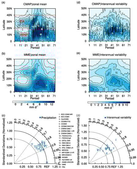
Figure 1.
Climatological and interannual variability of the seasonal migration of East Asian zonal mean (1979–2014, 115°–135° E) rainfall. Climate mean seasonal march for (a) Climate Precipitation Center Merged Analysis of Precipitation (CMAP), (b) multi-model ensemble (MME) (unit: mm day–1). (c) Taylor diagram exhibits a statistical comparison of the spatial structure of (a,b). The metrics encompass the standardized deviation ratios (SDR, referring to the ratio of model’s pattern standard deviation against the observed pattern standard deviation, vertical axis), root-mean-square-error (RMSE, distance to the REF), and the spatial pattern correlation coefficients (PCC, azimuthal axis) among the 21 CMIP6 models and MME mean comparing with the observation. (d–f) are the same as (a–c), but for the year-to-year standard deviations of the zonal mean rainfall.
The interannual variability is less skillful than the climatological seasonal cycle of the EA rainfall. Compared with the observation, although the simulated interannual standard deviation (SD) pattern is similar, the MME variabilities are much weaker over WP but stronger over EA (Figure 1d,e). Figure 1f shows the PCC score (0.88) of the interannual variability in MME is lower than the climatology in Figure 1c. In addition, the PCCs and the SDRs exhibit more vigorous spread amongst individual models. In general, the models with lower skill in climatology simulation also show lower interannual SD skills, such as the INM-CM4-8 and NorESM2-LM.
As to the annual cycle component, it is dominant in total rainfall over most EA sub-regions in either observation or CMIP6 models, particularly over tropical and subtropical monsoonal regions (Figure 2a,b). In observation, the annual cycle component explains more than 60% variance, except for the Tibetan Plateau and northwest China. Nevertheless, the CMIP6 MME result overestimates the contribution of the annual cycle (Figure 2b), implicating its overestimation of the annual cycle intensity. As such, the interannual variability is underestimated, presenting the attenuation of the high-frequency variances in the MME (Figure 1b). Comparing with the observation, the maximum of the annual cycle’s explained variances around the Yangtze River valley and the Bay of Bengal are different to some extent, resulting in a relatively lower PCC of 0.58. The individual models also cannot precisely reproduce the observed annual cycle domination, featured by the large diversity across them and the PCCs lower than 0.7 (Figure 2c). The pattern standard deviation of the models is higher than the observation as the majority of points falling outside the quadrant of radius one (i.e., SDR > 1).
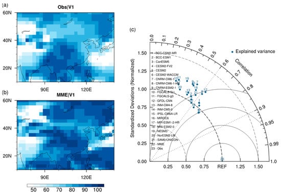
Figure 2.
The proportion of total variance explained by the annual cycle component of rainfall over East Asia (EA) (unit: %). (a) CMAP, (b) MME. (c) Taylor diagram for the explained variances.
Figure 3 displays the horizontal distribution of the gridded phase () and amplitude () of the annual cycle components. In observation, over the monsoon domain represents the peak of the summer monsoon rainy season. For instance, around June–July in India denotes the formation of the Indian summer monsoon in early summer (Figure 3a). The clockwise rotation of from April to late July over the South, Central, and North China in order indicates the seasonal migration of the EASM rainfall (Figure 1a). is large in the tropics but becomes small in mid-latitudes, consistent with the strong tropical monsoon convection but relevant weak rainfall of the EA summer monsoon (EASM). The annual cycle is further attenuated over the non-monsoon regions deep in the continent, where is much weaker.
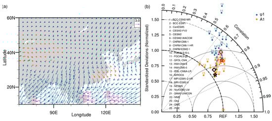
Figure 3.
Simulation on the spatial distribution of the gridded and of the annual cycle components over EA. (a) vector map for the annual cycle 73-pentad clock in observation (OBS) and MME. The length of the arrow quantifies the . The clockwise rotated vector with the northward vector indicates the at Julian pentad 1 and a total 73 pentads evenly distributed within 360°. The red, blue, purple, and green arrows represent the in spring, summer, autumn, and winter. The opaque and translucent arrows indicate the simulations and observations, respectively. (b) Multivariable Taylor diagram of the and of the annual cycle component. The star and diamond markers represent the GME and PME, as discussed later in Section 4.
In CMIP6 models, the MME results can generally capture the observed and over most areas, except for the dry inland region over Northwest China. In tropics, the CMIP6 models can basically reproduce the observed pattern of and , although the is larger in India but smaller over WNP. The difference of is considerable between simulation and observation, especially over the East and South China, and the South China Sea (SCS). The simulated is more identical than (Figure 4b). Moreover, the SDRs and the RMSEs of vary greatly among different models to indicate great challenge in simulating the phase of the annual cycle component. Meanwhile, the simulation biases between the two metrics are independent across the CMIP6 models. It implicates that a better simulated cannot guarantee a better simulation.
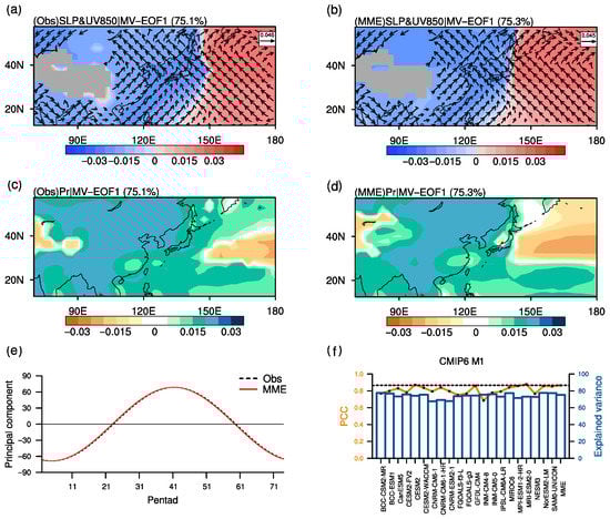
Figure 4.
First annual cycle mode (M1) of EA precipitation from MV-EOF1 in (a,c) OBS and (b,d) MME. (a,b) show the spatial structures for the SLP and 850-hPa horizontal wind anomalies and (c,d) for precipitation anomalies. The explained variance of M1 is 75.1% in observation and 75.3% in MME simulation. (e) Principal component (PC) time series of MV-EOF1. The horizontal axis ranges from Julian pentad 1 to 73. The black trigonometric function curve indicates the observation, and the red one indicates the MME mean. The amplitude and phase of the PC1 series are adopted as the amplitude () and phase () of M1. (f) Explained variances (blue bar) of MV-EOF1 in individual models and the MME mean. The MV-EOF is applied on the MME and individual models, respectively. The orange curve indicates the multivariate pattern correlation coefficients between the MV-EOF1 spatial pattern in OBS (a,c) and models (such as (b,d) for MME). The black dashed line indicates the MME PCC.
4. Modes of the Annual Cycle of East Asian Rainfall
Figure 4 shows the first dominant mode of the EAM annual cycle (hereafter referred to as M1), with the 75.1% explained variance in observation. Spatially, M1 presents the mature stage of the Asian summer monsoon. An anomalous large-scale low-pressure is located over the East Asian continent (Figure 4a). Meanwhile, a remarkable anomalous high-pressure emerges over the western Pacific, with the significant positive SLP and anticyclonic anomalies centered around 180° E. The continental low- and oceanic high- SLP constitutes an east–west seesaw pattern over the EA-WNP region. The SLP gradient maintains the large-scale monsoon rainfall over EA, which is uniformly enhanced over most moist regions with its maximum over the EA continent (Figure 4c). The PC1 exhibits the temporal evolution of M1, as shown by the black sinusoidal in Figure 4e. Thereafter, we calculate the amplitude () and phase () of the PC1 series. The value of is 68.6, and equals pentad 40.5, which around the summer solstice.
In general, the CMIP6 MME can reproduce the major characteristics of M1. The simulated zonal SLP gradient between land and ocean and the cyclonic and anticyclonic circulations in the lower troposphere are comparable to the observation (Figure 4c). The positive precipitation anomalies over most regions are reasonably reproduced in simulations (Figure 4d), though some deficiencies exist at the high-latitude Pacific Ocean, South China, and tropical WNP. The amplitude and phase of the simulated PC1 are 68.7 and pentad 40.2, respectively, close to the observation. The M1 is consistently stable among the 21 individual models (Figure 4f). The explained variance of M1 in each model is around 75%, which is close to the observation and the MME result (75.3%). The relative high PCC score between the simulated and observed pattern of M1 (0.86 for MME) shows a small inter-model spread (ranging between 0.68 and 0.88, and 0.049 for the inter-model standard deviation).
Figure 5 depicts the situation of the second annual cycle mode (M2) of the EA rainfall. M2 explained the variance of 24.9% in observation. A strong east-west SLP gradient exists in the low-latitudes, whose positive (negative) center is located over WNP (the Southeast of Tibetan Plateau). A relatively weak cyclone maintains on the ocean to the east of Japan. The precipitation in M2 is above-normal from South China to the adjacent oceans south of Japan beneath a couple of anticyclonic and cyclonic. In comparison, the rainfall is below-normal over most of the oceans (Figure 5c). The mature phase of M2 ( = pentad 22.3) is close to the spring equinox, exactly corresponding to the spring rainy season in South China (Figure 5e).
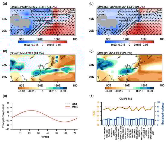
Figure 5.
Second annual cycle mode (M2) from MV-EOF2 in (a,c) OBS and (b,d) MME. (a,b) show the spatial structures for the SLP and 850-hPa horizontal wind anomalies and (c,d) for precipitation anomalies. The explained variance of M2 is 24.9% in observation and 24.7% in MME simulation. (e) PC time series of MV-EOF2. The black trigonometric function curve indicates the observation, and the red one indicates the MME mean. (f) Explained variances (blue bar) of MV-EOF2 in individual models and the MME mean. The orange curve indicates the multivariate pattern correlation coefficients between the MV-EOF2 spatial pattern in OBS (a,c) and models (such as (b,d) for MME). The black dashed line indicates the MME PCC.
The M2 in the MME simulations has an explained variance of 24.7%. The positive (negative) SLP anomalies and anomalous anticyclone (cyclone) in tropics resemble the observations, although the cyclone over the ocean to the east of Japan is slightly stronger. The spatial distribution of the precipitation anomalies is reasonably reproduced, except that the above-normal anomalies of precipitation are overestimated in South China but underestimated in the southeast of Japan. The mature phase of the simulated PC2 emerges in pentad 22.0 and closes to the observation (Figure 5e). For the individual models, the performance of M2 is ragged among them. The PCCs ranging from 0.64 to 0.80 vary largely among the models. The inter-model standard deviation of the PCC is 0.057, suggesting a broad simulation diversity in M2.
The reproducibility of the M1 is mainly ascribed to simulation among the models (Figure 3b). Models that better reproduce could simulate a more realistic M1 (e.g., the GFDL-CM4, MPI-ESM1-2-HR, and NorESM2-LM). However, both M1 and M2 are profoundly related to the simulation performance (Figure not shown), resulting in the considerable challenge of the simulation on the annual cycle phase. Spatially, the sub-regions with larger biases of and also show lower skills in the pattern of M1 and M2 (e.g., South China and SCS).
To examine the temporal stability of the simulated annual cycle modes, we first divide the HIST (1850–2014) experiment into 14 groups. Each group has a period of 30 years starting from 1850 to 1979 with an interval of 10 years. Afterward, the MV-EOF is conducted repeatedly on each group to check their similarity. The results show that the relative contribution of M1 and M2 to the annual cycle component is constant, and the proportion does not broadly vary with the sliding of the modelled climatology. The explained variance ratios of M1 to M2 stay at ~3.1 in the MME simulation (Figure 6a), as well as the ensemble members, albeit the existence of the inter-model spread (blue shading). The PCCs of M1 and M2 pattern are sufficiently high between each episode and the standard period (1979–2014), especially the MME result (Figure 6b). The comparative results show that M1 is more stable than M2. Thereby, the annual cycle modes are temporal stable in the longtime historical experiments.
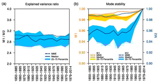
Figure 6.
Mode stability during different modelled climatology among all the models. (a) Ratios of the explained variance of M1 to M2 in individual models and the MME mean. The horizontal axis represents 14 sliding modelled climatology covering the period from 1850 to 2014. (b) The PCCs between the MV-EOF pattern for 1979–2014 climatology and the pattern during different climatology. The dash curves in (a) and (b) refers to the MME results. The solid curves and blue shadings indicate the median and the 25- to 75-percentiles of the 21 models.
Since the M1 and M2 are stable among individual CMIP6 models, resemble the observation, and not sensitive to the temporal variation, we can project the simulated results onto the observed modes to reconstruct the PCs (i.e., projected PC1 and PC2) and make a unified comparison. This is a commonly used strategy under the precondition of finding a stable projection basis (e.g., the MJO [64,65]). The amplitudes of the projected PC1 (abbreviated to ) share significant common biases across the models, consistent with the systematic bias in the monsoon intensity (Figure 1b). All the simulations are weaker than the observations, though the MME result performs better (Figure 7a). The projected phase in simulation () is either slightly lead or lag the observations (Figure 7c). Most models can reproduce the timing of the mature phase with the biases less than 1.5 pentads, except for the CESM2-FV2 (1.81 pentads phase delay) and CESM2-WACCM (1.58 pentads phase delay). Some models (CNRM-CM6-1, CNRM-CM6-1-HR, CNRM-ESM2-1, INM-CM5-0, and MRI-ESM2-0) can accurately simulate the , which is beyond the MME simulation (0.27 pentads phase delay). The inter-model standard deviation of biases is 0.82 pentads.
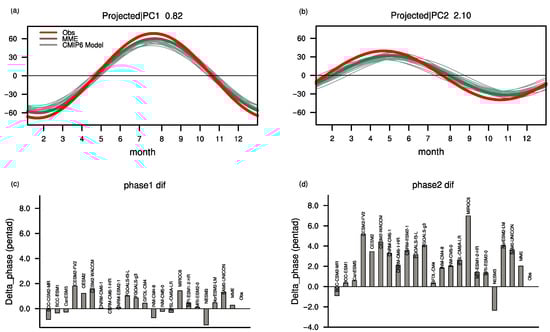
Figure 7.
Projection principal component series (projected PCs) onto the observed (a) annual cycle M1 and (b) M2. The red, green, and gray curves represent the projected PCs in the observation, MME mean, and individual models, respectively. The timing of the maximum equal to the phase of trigonometric functions, which indicates the projected phase of the annual cycle mode in simulations. (c,d) Phase biases for M1 and M2. The phase biases are measured by the mathematic difference of maximum timing between the simulations and observations in (a,b). The sub-title numbers in (a,b) represent the inter-model standard deviations of the phase biases for M1 (0.82) and M2 (2.10).
The amplitudes of projected PC2 () are also weaker in all the simulations, as shown in Figure 7b. Although the value is relatively low, the inter-model diversity is comparable with the . The MME result is outperforming than most individual models. The differences between the projected PC2 phase () and the observation suggest a great spread among the ensemble models (Figure 7d). The inter-model standard deviation of the phase biases reaches 2.10 pentads, evidently larger than the counterpart in projected PC1 (0.82). Nearly all the models (except for the BCC-CSM2-MR and NESM3) present a tremendous lagging bias, indicating that the temporal evolution is systematically delayed compared to the observations. Some models even suffer more than four pentads (beyond double M1) phase delay, alongside a maximum up to 6.99 pentads in the MIROC6. Fortunately, some models (BCC-CSM2-MR, BCC-ESM1, CanESM5, GFDL-CM4, INM-CM4-8, MPI-ESM1-2-HR, and MRI-ESM2-0) feature the phase delay less than two pentads and the MME result (2.03 pentad delay), especially the BCC-ESM1 and GFDL-CM4 with only 0.35 and 0.33, respectively.
Considering the underlying physical mechanism of the two modes represents the dominant features of the EA annual cycle. The phase biases are essential for the mode accuracy. It is vital that idealized models reasonably reproduce the phases in both of them. Thereby, we pick out the optimized subset of good performing models (GMs, include the BCC-ESM1, CanESM5, and GFDL-CM4) in annual cycle modes according to the ranking of the sum of phase biases in Figure 7c,d (sum < 1 pentad, choosing one model from the same host center). These models share relatively small phase biases of M1(<1 pentad) and M2 (<2 pentads). In contrast, the MIROC6, CESM2-FV2, and Fgoals-g3 are categorized as the poor performance models (PMs) with the most significant phase biases, especially the phase delay on M2.
More challenging in climate models, the annual cycle varies substantially year by year and exhibits prominent interannual variations. In the following, we project the annual cycle component of every year onto the observed M1 and M2. Every single year has its projected amplitude () and phase () of the annual cycle modes. Hence, we obtain the interannual standard deviations (ISDs) of the and in individual models, as shown in Figure 8. In general, the simulated interannual variations of the amplitude are relatively weak compared to the observation, as the scaled ISDs below the reference line, especially the amplitude of M2. On the other hand, the simulations of the phase ISD are mostly higher than the observations. Nearly all the models overestimate the phase ISD of M1, and half models overestimate the phase ISD of M2. Some reproduce all four ISDs relatively well. Examples are the BCC-ESM1, GFDL-CM4, BCC-CSM2-MR, and INM-CM5-0, which also considerably capture the climatological annual cycle mode (Figure 7). In contrast, models with the low accuracy of the climatology (e.g., CESM2-FV2, CNRM-ESM2-1, and NorESM2-LM) tend to exhibit notable biases in ISD.
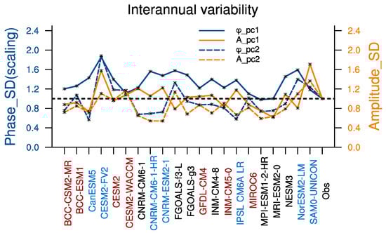
Figure 8.
Interannual variabilities of the projected amplitude () and phase () of the annual cycle modes. The solid and dashed curves represent the interannual standard deviations (ISDs) of M1 and M2, respectively. The orange and dark blue curves represent the ISDs of the projected amplitude and phase. The ISDs for the individual models are scaled by the corresponding values in the observations. The dashed black line indicates the ISDs in observation (=1.0 after scaled). The red (blue) tick marks of abscissa represent the relative good (bad) four ISDs performances which close (departure) to the observed ISDs (dashed black line).
In summary, the GMs well reproduce the annual cycle modes in climatology and interannual variations, with evident lower phase biases in M1 and M2 than the PMs, thus reasonably capturing the underlying physics related to the key process in the EAM evolution. Moreover, as shown in Figure 3b, the ensemble of the GMs (GME) simulates the continental-scale annual cycle components (i.e., higher skill in and ) more reliable than the PMs (PME) and on par with the MME. These results verify the benchmark that models with fewer phase errors in annual cycle modes tend to represent more realistic annual cycle features over East Asia.
5. Concluding Remarks
5.1. Summary
This study documents evaluation against observations of the simulation of the annual cycle over the EAM domain, using the new simulations of the 21 released CMIP6 CGCMs HIST. We propose a robust quantification and benchmark of the annual cycle of East Asian rainfall in climate models. The main conclusions are as follows:
Initially, CMIP6 models yield the basic veracity while still sharing considerable limitations in representing the climatological annual cycle’s unique features in East Asia, especially the annual cycle phase. The notable discrepancies mainly exist in East and South China, and the South China Sea.
We propose a new assessing benchmark by utilizing the annual cycle’s EOF modes (M1 and M2), which embed the underlying physics associated with the EAM annual evolution. The MME simulations can generally reproduce the main characteristics of the annual cycle modes, while still suffering some drawbacks. First, the amplitudes of both annual cycle modes exhibit significant common biases across the models. Second, although most models can reproduce the M1 phase’s timing with the phase biases less than 1.5 pentads, nearly all the models represent a prominent delayed phase of M2, some even beyond four pentads.
Finally, according to the combined phase biases of M1 and M2, the BCC-ESM1, CanESM5, and GFDL-CM4 are defined as the best performing models (GMs). The GMs’ ensemble can capture the phase of the annual cycle modes that link to the critical process of the EAM evolution driving by the external forcing. They can also reproduce the spatiotemporal structures of the annual cycle reasonably well. Moreover, the models capture the annual cycle modes in climatology commonly perform better interannual variabilities and vice versa. These results suggest the necessity of reasonable annual cycle mode simulation. Therefore, the dominant modes of the EAM annual cycle can act as the evaluate benchmark in the EAM modelling framework, providing valuable insight into the bias correction strategies for decreasing the uncertainty in the simulation of the EAM.
5.2. Discussion
What causes the limits and deficiencies in representing the annual cycle modes and the excellent model spread calls for further investigation and beyond our study. The multistage evolution and annual cycle of rainfall over East Asia correspond with the surface boundary forcing (e.g., SST, snow cover, and soil moisture) and internal atmospheric variabilities in observations. It is foreseeable that annual cycle of the monsoon system links with complicated and various modelling factors, including the mean state and cycle of the sea surface temperature (SST), mid-latitude processes, physical parameterizations, dynamic core, among others. For instance, previous works have suggested that both the mean state and the cyclic progression of the SST warming profoundly affects the seasonal delay of the tropical rainfall [66,67,68]. In climate models, the annual cycle SST contributes to the annual cycle rainfall bias in some regions [69]. In addition, SST anomalies associated with the El Niño—Southern Oscillation (ENSO) considerably impact the East Asian monsoon. Therefore, the realistic simulation of these SST anomalies, including the absolute magnitude and temporal behavior, might play a crucial role in this issue.
As shown in Figure 7, comparing a subset of models (CNRM-CM6-1, CNRM-CM6-1-HR, and CNRM-ESM2-1) with different atmospheric horizontal resolutions, the high-resolution one shows better performance. In addition, most of the Earth system models we used also exhibit relatively low phase biases. The extent to which the model resolution and complexity can influence the annual cycle over East Asia requires further explorations. In our work, we only use one ensemble member for each model, ignoring the atmospheric internal variabilities. How does the internal variability impact the simulation of the East Asian annual cycle?
In any event, many future avenues deserve in-depth research. Despite all puzzles and challenges, it is crucial to identify the possible vital factors for modelling community. Given the annual cycle is the fundamental feature of the EAM system. Reliable simulation is crucial for society and adaptation strategies under climate change. Our analysis highlights a crucial model bias to keep in mind for future work on EAM modelling. The capacity to accurately simulate the distribution and timing of East Asian rainfall would appear to be a necessary precursor to making reliable predictions for the watershed, agricultural, and hydrological purposes.
Author Contributions
Conceptualization, C.Z. and B.L.; data curation, Y.Y. and S.J.; formal analysis, Y.Y.; investigation, Y.Y., C.Z., and B.L.; methodology, Y.Y., C.Z., and B.L.; software, Y.Y. and S.J.; visualization, Y.Y., C.Z., and B.L.; writing—original draft, Y.Y.; writing—review and editing, Y.Y., C.Z., and B.L. All authors have read and agreed to the published version of the manuscript.
Funding
This work was jointly funded by the National Natural Science Foundation of China (42005131, 41830969), the National Key R&D Program (2018YFC1505904), supported by The Second Tibetan Plateau Scientific Expedition and Research (STEP) program (grant no. 2019QZKK0105), and the Basic Scientific Research and Operation Foundation of the Chinese Academy of Meteorological Sciences (CAMS) under grant 2018Z006, the scientific development foundation of CAMS (2020KJ012). This study was also supported by the Jiangsu Collaborative Innovation Center for Climate Change.
Institutional Review Board Statement
Not applicable.
Informed Consent Statement
Not applicable.
Data Availability Statement
Publicly available datasets were analyzed in this study. These datasets are freely available through the Earth System Grid Federation: https://esgf-node.llnl.gov/search/cmip6.
Acknowledgments
We thank the four anonymous reviewers for their constructive comments. We acknowledge the World Climate Research Programme’s Working Group on Coupled Modelling, which is responsible for CMIP, and we thank the climate modeling groups (listed in Table 1 of this paper) for producing and making available their model output. For CMIP, the U.S. Department of Energy’s Program for Climate Model Diagnosis and Intercomparison provides coordinating support and led development of software infrastructure in partnership with the Global Organization for Earth System Science Portals.
Conflicts of Interest
The authors declare that they have no conflict of interest.
References
- Field, C.; Barros, V.; Dokken, D.; Mach, K.; Mastrandrea, M.; Mastrandrea, P.; White, L. Intergovernmental panel on climate change. Climate change 2014: Impacts, adaptation, and vulnerability. In Contribution of Working Group II to the Fifth Assessment Report of the Intergovernmental Panel on Climate Change; Cambridge University Press: Cambridge, UK, 2014. [Google Scholar]
- Trenberth, K.E.; Stepaniak, D.P.; Caron, J.M. The global monsoon as seen through the divergent atmospheric circulation. J. Clim. 2000, 13, 3969–3993. [Google Scholar] [CrossRef]
- Wang, B.; Ding, Q. Global monsoon: Dominant mode of annual variation in the tropics. Dynam Atmos Ocean. 2008, 44, 165–183. [Google Scholar] [CrossRef]
- Wang, B.; Liu, J.; Kim, H.J.; Webster, P.J.; Yim, S.Y. Recent change of the global monsoon precipitation (1979–2008). Clim. Dyn. 2012, 39, 1123–1135. [Google Scholar] [CrossRef]
- Wang, P.X.; Wang, B.; Cheng, H.; Fasullo, J.; Guo, Z.T.; Kiefer, T.; Liu, Z.Y. The global monsoon across time scales: Mechanisms and outstanding issues. Earth Sci. Rev. 2017, 174, 84–121. [Google Scholar] [CrossRef]
- Wang, B.; Lin, H. Rainy season of the Asian-Pacific summer monsoon. J. Clim. 2002, 15, 386–398. [Google Scholar] [CrossRef]
- Endo, H.; Kitoh, A. Projecting changes of the Asian summer monsoon through the twenty-first century. In The Monsoons and Climate Change; Springer: Berlin/Heidelberg, Germany, 2016; pp. 47–66. [Google Scholar]
- Hsu, H.H.; Zhou, T.J.; Matsumoto, J. East Asian, Indochina and Western North Pacific summer monsoon—An update. Asia Pac. J. Atmos. Sci. 2014, 50, 45–68. [Google Scholar] [CrossRef]
- Chen, J.Q.; Bordoni, S. Orographic effects of the Tibetan Plateau on the East Asian summer monsoon: An energetic perspective. J. Clim. 2014, 27, 3052–3072. [Google Scholar] [CrossRef]
- Liu, X.D.; Yin, Z.Y. Sensitivity of East Asian monsoon climate to the uplift of the Tibetan Plateau. Palaeogeogr. Palaeocl. 2002, 183, 223–245. [Google Scholar] [CrossRef]
- Wu, G.X.; Liu, Y.M.; He, B.; Bao, Q.; Duan, A.M.; Jin, F.F. Thermal controls on the Asian summer monsoon. Sci. Rep. UK 2012, 2. [Google Scholar] [CrossRef]
- Yanai, M.; Li, C.; Song, Z. Seasonal heating of the Tibetan Plateau and its effects on the evolution of the Asian summer monsoon. J. Meteorol. Soc. Jpn. Ser. II 1992, 70, 319–351. [Google Scholar] [CrossRef]
- Ye, D. Some characteristics of the summer circulation over the Qinghai-Xizang (Tibet) Plateau and its neighborhood. B Am. Meteorol. Soc. 1981, 62, 14–19. [Google Scholar] [CrossRef]
- Chen, C.S.; Chen, Y.L. The rainfall characteristics of Taiwan. Mon. Weather Rev. 2003, 131, 1323–1341. [Google Scholar] [CrossRef]
- Chen, C.A.; Hsu, H.H.; Hong, C.C.; Chiu, P.G.; Tu, C.Y.; Lin, S.J.; Kitoh, A. Seasonal precipitation change in the Western North Pacific and East Asia under global warming in two high-resolution AGCMs. Clim. Dyn. 2019, 53, 5583–5605. [Google Scholar] [CrossRef]
- Chou, C.; Huang, L.F.; Tseng, L.S.; Tu, J.Y.; Tan, P.H. Annual cycle of rainfall in the Western North Pacific and East Asian sector. J. Clim. 2009, 22, 2073–2094. [Google Scholar] [CrossRef]
- Lin, H.; Wang, B. The time-space structure of the Asian-Pacific summer monsoon: A fast annual cycle view. J. Clim. 2002, 15, 2001–2019. [Google Scholar] [CrossRef]
- Hsu, H.H.; Terng, C.T.; Chen, C.T. Evolution of large-scale circulation and heating during the first transition of Asian summer monsoon. J. Clim. 1999, 12, 793–810. [Google Scholar] [CrossRef]
- Hung, C.W.; Hsu, H.H. The first transition of the Asian summer monsoon, intraseasonal oscillation, and Taiwan mei-yu. J. Clim. 2008, 21, 1552–1568. [Google Scholar] [CrossRef]
- Ueda, H.; Yasunari, T.; Kawamura, R. Abrupt seasonal change of large-scale convective activity over the western Pacific in the northern summer. J. Meteorol. Soc. Jpn. Ser. II 1995, 73, 795–809. [Google Scholar] [CrossRef][Green Version]
- Wu, R.; Wang, B. Multi-stage onset of the summer monsoon over the western North Pacific. Clim. Dyn. 2001, 17, 277–289. [Google Scholar] [CrossRef]
- Lee, B.S. A synoptic study of the early summer and autumn rainy season in Korea and in East Asia. Geogr. Rep. Tokyo Metrop. Univ. 1974, 9, 79–95. [Google Scholar]
- Tian, S.F.; Yasunari, T. Climatological aspects and mechanism of spring persistent rains over central China. J. Meteorol. Soc. Jpn. Ser. II 1998, 76, 57–71. [Google Scholar] [CrossRef]
- Wan, R.J.; Wang, T.M.; Wu, G.X. Temporal variations of the spring persistent rains and South China Sea sub-high and their correlations to the circulation and precipitation of the East Asian summer monsoon. Acta Meteorol. Sin. 2008, 22, 530–537. [Google Scholar]
- Wang, B.; Jhun, J.G.; Moon, B.K. Variability and singularity of Seoul, South Korea, rainy season (1778–2004). J. Clim. 2007, 20, 2572–2580. [Google Scholar] [CrossRef]
- Ding, Y.H.; Chan, J.C.L. The East Asian summer monsoon: An overview. Meteorol. Atmos. Phys. 2005, 89, 117–142. [Google Scholar]
- Lau, K.; Yang, G.; Shen, S. Seasonal and intraseasonal climatology of summer monsoon rainfall over Eeat Asia. Mon. Weather Rev. 1988, 116, 18–37. [Google Scholar] [CrossRef]
- Tao, S.Y.; Chen, L.X. A review of recent research on the East Asian summer monsoon in China. In Monsoon Meteorology; Oxford University Press: London, UK, 1987; Volume 1987, pp. 60–92. [Google Scholar]
- Kusunoki, S.; Arakawa, O. Are CMIP5 models better than CMIP3 models in simulating precipitation over East Asia? J. Clim. 2015, 28, 5601–5621. [Google Scholar] [CrossRef]
- Liang, X.Z.; Wang, W.C.; Samel, A. Biases in AMIP model simulations of the east China monsoon system. Clim. Dyn. 2001, 17, 291–304. [Google Scholar] [CrossRef]
- Ma, L.B.; Zhu, Z.W.; Li, J.; Cao, J. Improving the simulation of the climatology of the East Asian summer monsoon by coupling the Stochastic Multicloud Model to the ECHAM6.3 atmosphere model. Clim. Dyn. 2019, 53, 2061–2081. [Google Scholar] [CrossRef]
- Song, F.F.; Zhou, T.J. The climatology and interannual variability of East Asian summer monsoon in CMIP5 coupled models: Does air-sea coupling improve the simulations? J. Clim. 2014, 27, 8761–8777. [Google Scholar] [CrossRef]
- Webster, P.J.; Magana, V.O.; Palmer, T.; Shukla, J.; Tomas, R.; Yanai, M.; Yasunari, T. Monsoons: Processes, predictability, and the prospects for prediction. J. Geophys. Res. Ocean. 1998, 103, 14451–14510. [Google Scholar] [CrossRef]
- Boo, K.O.; Martin, G.; Sellar, A.; Senior, C.; Byun, Y.H. Evaluating the East Asian monsoon simulation in climate models. J. Geophys. Res. Atmos. 2011, 116. [Google Scholar] [CrossRef]
- Huang, D.Q.; Zhu, J.; Zhang, Y.C.; Huang, A.N. Uncertainties on the simulated summer precipitation over Eastern China from the CMIP5 models. J. Geophys. Res. Atmos. 2013, 118, 9035–9047. [Google Scholar] [CrossRef]
- Kang, I.S.; Jin, K.; Wang, B.; Lau, K.M.; Shukla, J.; Krishnamurthy, V.; Schubert, S.D.; Wailser, D.E.; Stern, W.F.; Kitoh, A.; et al. Intercomparison of the climatological variations of Asian summer monsoon precipitation simulated by 10 GCMs. Clim. Dyn. 2002, 19, 383–395. [Google Scholar]
- Kripalani, R.H.; Oh, J.H.; Chaudhari, H.S. Response of the East Asian summer monsoon to doubled atmospheric CO2: Coupled climate model simulations and projections under IPCC AR4. Appl. Clim. 2007, 87, 1–28. [Google Scholar] [CrossRef]
- Sperber, K.; Annamalai, H.; Kang, I.S.; Kitoh, A.; Moise, A.; Turner, A.; Wang, B.; Zhou, T. The Asian summer monsoon: An intercomparison of CMIP5 vs. CMIP3 simulations of the late 20th century. Clim. Dyn. 2013, 41, 2711–2744. [Google Scholar] [CrossRef]
- Lee, J.W.; Hong, S.Y.; Chang, E.C.; Suh, M.S.; Kang, H.S. Assessment of future climate change over East Asia due to the RCP scenarios downscaled by GRIMs-RMP. Clim. Dyn. 2013, 42, 733–747. [Google Scholar] [CrossRef]
- Lambert, S.J.; Boer, G.J. CMIP1 evaluation and intercomparison of coupled climate models. Clim. Dyn. 2001, 17, 83–106. [Google Scholar] [CrossRef]
- Yao, J.C.; Zhou, T.J.; Guo, Z.; Chen, X.L.; Zou, L.W.; Sun, Y. Improved performance of high-resolution atmospheric models in simulating the East Asian summer monsoon rain belt. J. Clim. 2017, 30, 8825–8840. [Google Scholar] [CrossRef]
- Gong, H.N.; Wang, L.; Chen, W.; Wu, R.G.; Wei, K.; Cui, X.F. The climatology and interannual variability of the East Asian winter monsoon in CMIP5 models. J. Clim. 2014, 27, 1659–1678. [Google Scholar] [CrossRef]
- Jiang, D.B.; Wang, H.J.; Lang, X.M. Evaluation of East Asian climatology as simulated by seven coupled models. Adv. Atmos. Sci. 2005, 22, 479–495. [Google Scholar]
- Min, S.K.; Park, E.H.; Kwon, W.T. Future projections of East Asian climate change from multi-AOGCM ensembles of IPCCSRES scenario simulations. J. Meteorol. Soc. Jpn 2004, 82, 1187–1211. [Google Scholar] [CrossRef]
- Zhang, J.; Li, L.; Zhou, T.J.; Xin, X.G. Evaluation of spring persistent rainfall over East Asia in CMIP3/CMIP5 AGCM simulations. Adv. Atmos. Sci. 2013, 30, 1587–1600. [Google Scholar] [CrossRef]
- Zhao, P.; Jiang, P.P.; Zhou, X.J.; Zhu, C.W. Modeling impacts of East Asian Ocean-Land thermal contrast on spring southwesterly winds and rainfall in eastern China. Chin. Sci. Bull. 2009, 54, 4733–4741. [Google Scholar] [CrossRef][Green Version]
- Kitoh, A.; Uchiyama, T. Changes in onset and withdrawal of the East Asian summer rainy season by multi-model global warming experiments. J. Meteorol. Soc. Jpn 2006, 84, 247–258. [Google Scholar] [CrossRef]
- Kai, T.; Zhong-Wei, Y.; Xue-Bin, Z.; Wen-Jie, D. Simulation of precipitation in monsoon regions of China by CMIP3 models. Atmos. Ocean. Sci. Lett. 2009, 2, 194–200. [Google Scholar] [CrossRef]
- Yu, R.C.; Li, W.; Zhang, X.H.; Liu, Y.M.; Yu, Y.Q.; Liu, H.L.; Zhou, T.J. Climatic features related to eastern China summer rainfalls in the NCAR CCM3. Adv. Atmos. Sci. 2000, 17, 503–518. [Google Scholar]
- Eyring, V.; Bony, S.; Meehl, G.A.; Senior, C.A.; Stevens, B.; Stouffer, R.J.; Taylor, K.E. Overview of the Coupled Model Intercomparison Project Phase 6 (CMIP6) experimental design and organization. Geosci. Model Dev. 2016, 9, 1937–1958. [Google Scholar] [CrossRef]
- Jiang, D.B.; Hu, D.; Tian, Z.; Lang, X. Differences between CMIP6 and CMIP5 models in simulating climate over China and the East Asian monsoon. Adv. Atmos. Sci. 2020, 37, 1102–1118. [Google Scholar] [CrossRef]
- Wang, B.; Jin, C.; Liu, J. Understanding future change of global monsoons projected by CMIP6 models. J. Clim. 2020, 33, 6471–6489. [Google Scholar] [CrossRef]
- Xin, X.; Wu, T.; Zhang, J.; Yao, J.; Fang, Y. Comparison of CMIP6 and CMIP5 simulations of precipitation in China and the East Asian summer monsoon. Int. J. Clim. 2020. [Google Scholar] [CrossRef]
- Xie, P.; Arkin, P.A. Global precipitation: A 17-year monthly analysis based on gauge observations, satellite estimates, and numerical model outputs. B Am. Meteorol. Soc. 1997, 78, 2539–2558. [Google Scholar] [CrossRef]
- Kanamitsu, M.; Ebisuzaki, W.; Woollen, J.; Yang, S.-K.; Hnilo, J.; Fiorino, M.; Potter, G. NCEP–DOE AMIP-II Reanalysis (R-2). B Am. Meteorol. Soc. 2002, 83, 1631–1644. [Google Scholar] [CrossRef]
- Taylor, K.E. Summarizing multiple aspects of model performance in a single diagram. J. Geophys. Res. Atmos. 2001, 106, 7183–7192. [Google Scholar] [CrossRef]
- Ha, K.J.; Moon, S.; Timmermann, A.; Kim, D. Future changes of summer monsoon characteristics and evaporative demand over Asia in CMIP6 simulations. Geophys Res. Lett. 2020, 47. [Google Scholar] [CrossRef]
- Horn, L.H.; Bryson, R.A. Harmonic analysis of the annual march of precipitation over the united states. Ann. Assoc. Am. Geogr. 1960, 50, 157–171. [Google Scholar] [CrossRef]
- Bombardi, R.J.; Kinter, J.L.; Frauenfeld, O.W. A global gridded dataset of the characteristics of the rainy and dry seasons. B Am. Meteorol. Soc. 2019, 100, 1315–1328. [Google Scholar] [CrossRef]
- Boyle, S.J. Evaluation of the annual cycle of precipitation over the United States in GCMs: AMIP simulations. J. Clim. 1998, 11, 1041–1055. [Google Scholar] [CrossRef]
- Dunning, C.M.; Black, E.C.L.; Allan, R.P. The onset and cessation of seasonal rainfall over Africa. J. Geophys. Res. Atmos. 2016, 121, 11405–11424. [Google Scholar] [CrossRef]
- Martin, D.W.; Hinton, B.B. Annual cycle in rainfall of the Indo-Pacific region. J. Clim. 1999, 12, 1240–1256. [Google Scholar] [CrossRef]
- Jiang, S.; Zhu, C.W.; Jiang, N. Variations in the annual cycle of the East Asian monsoon and its phase-induced interseasonal rainfall anomalies in China. Atmos. Ocean. Sci. Lett. 2020, 1–7. [Google Scholar] [CrossRef]
- Brunet, G.; Lin, H.; Derome, J. Forecast Skill of the Madden–Julian Oscillation in Two Canadian Atmospheric Models. Mon. Weather Rev. 2008, 136, 4130–4149. [Google Scholar] [CrossRef]
- Klingaman, N.P.; Woolnough, S.J. The role of air-sea coupling in the simulation of the Madden-Julian oscillation in the Hadley Centre model. Q. J. Roy Meteor. Soc. 2014, 140, 2272–2286. [Google Scholar] [CrossRef]
- Dwyer, J.G.; Biasutti, M.; Sobel, A.H. The effect of greenhouse gas–induced changes in SST on the annual cycle of zonal mean tropical precipitation. J. Clim. 2014, 27, 4544–4565. [Google Scholar] [CrossRef]
- Biasutti, M.; Sobel, A.H. Delayed Sahel rainfall and global seasonal cycle in a warmer climate. Geophys. Res. Lett. 2009, 36. [Google Scholar] [CrossRef]
- Song, F.; Leung, L.R.; Lu, J.; Dong, L. Seasonally dependent responses of subtropical highs and tropical rainfall to anthropogenic warming. Nat. Clim. Chang. 2018, 8, 787–792. [Google Scholar] [CrossRef]
- Biasutti, M.; Battisti, D.S.; Sarachik, E. Mechanisms controlling the annual cycle of precipitation in the tropical Atlantic sector in an atmospheric GCM. J. Clim. 2004, 17, 4708–4723. [Google Scholar] [CrossRef]
Publisher’s Note: MDPI stays neutral with regard to jurisdictional claims in published maps and institutional affiliations. |
© 2020 by the authors. Licensee MDPI, Basel, Switzerland. This article is an open access article distributed under the terms and conditions of the Creative Commons Attribution (CC BY) license (http://creativecommons.org/licenses/by/4.0/).