Resolution Dependence of Turbulent Structures in Convective Boundary Layer Simulations

Abstract

Large-eddy simulations are performed using the U.K. Met Office Large Eddy Model to study the effects of resolution on turbulent structures in a convective boundary layer. A standard Smagorinsky subgrid scheme is used. As the grid length is increased, the diagnosed height of the boundary layer increases, and the horizontally- and temporally-averaged temperature near the surface and in the inversion layer increase. At the highest resolution, quadrant analysis shows that the majority of events in the lower boundary layer are associated with cold descending air, followed by warm ascending air. The largest contribution to the total heat flux is made by warm ascending air, with associated strong thermals. At lower resolutions, the contribution to the heat flux from cold descending air is increased, and that from cold ascending air is reduced in the lower boundary layer; around the inversion layer, however, the contribution from cold ascending air is increased. Calculations of the heating rate show that the differences in cold ascending air are responsible for the warm bias below the boundary layer top in the low resolution simulations. Correlation length and time scales for coherent resolved structures increase with increasing grid coarseness. The results overall suggest that differences in the simulations are due to weaker mixing between thermals and their environment at lower resolutions. Some simple numerical experiments are performed to increase the mixing in the lower resolution simulations and to investigate backscatter. Such simulations are successful at reducing the contribution of cold ascending air to the heat flux just below the inversion, although the effects in the lower boundary layer are weaker.

1. Introduction

The development of high resolution numerical weather prediction (NWP) [1] models has brought into sharp focus the appropriateness of existing boundary layer subgrid schemes. The atmospheric boundary layer is the lowest part of the troposphere, which responds quickly to surface forcing [2]. It is generally characterised by stable and unstable conditions respectively at night and during the day, with a clear diurnal cycle over land. The top of the day-time convective boundary layer (CBL) is marked by an inversion layer, the height $z_i$ of which constrains the size of the largest energy-containing eddies l∼$z_i$. Column-based parametrization schemes for boundary layer turbulence were designed for relatively low resolution NWP simulations and assume that the horizontal grid spacing Δ is much larger than l. This approximation is no longer valid for the simulation of the CBL with the latest NWP models [3], which operate with $\Delta$ on the order of 1 km or less (e.g., [4,5,6]). Grid lengths of order of hundreds of metres mean that the turbulence is partially resolved, being in the regime of “coarse-grid” large eddy simulations (LES); the coarser end of this regime is sometimes called the “grey zone” or “terra incognita” [7,8,9]. Modellers need to address two key questions: (i) How physically realistic is the resolved turbulence? (ii) What compensating adjustments need be made to the parametrization of the subgrid turbulence?

Addressing these questions relies on the availability of a “truth” reference to compare against. A sufficiently high resolution LES can be used for this purpose [9]. Wurps et al. [10] found grid lengths of $2.5$ m, 10 m and 20 m to be sufficient to resolve the stable, neutral and CBL structures, respectively. Other studies [11,12] have shown that large eddy simulations of a CBL can be considered to be well resolved with a grid length of 25 m or less, while Park et al. [13] found a grid spacing of 20 m to be sufficient to study the decaying CBL. Using grid lengths of 80 m, 40 m, 20 m and 10 m, Matheou and Chung [14] concluded that an adequate grid length depends on the diagnostic of interest. They found the boundary layer height to be the same for all grid lengths used, and turbulent kinetic energy (TKE) converged for $\Delta \le 20$ m. Matheou et al. [15] also found grid convergence for $\Delta \le 20$ m when simulating shallow cumulus convection, although they noted that this finding cannot be extended to precipitating clouds.

Sullivan and Patton [11] examined second-order statistics, energy spectra and entrainment statistics from the LES of a CBL at a range of horizontal grid spacing $\Delta$ from 160 m to 5 m; they found grid independence in the interior of the boundary layer ($0.1<z/z_i<0.9$, for $\Delta \le 20$ m. The authors also depicted the structure of the vertical velocity field at different heights. They found convergence at the corners of hexagonal patterns in the surface layer giving rise to strong updraughts evolving into large plumes near the BL top. They also showed smaller scale vortices resembling dust devils, whose detailed dynamics may not be captured at coarser resolutions. A detailed study of the impact of grid spacing on coherent resolved structures remains to be done and will be our focus here.

The existence of coherent structures extending through the boundary layer is a dominant feature that drives mixing throughout the CBL. Comparisons from LES with and without an imposed shear reveal differences in the resulting boundary layer structure. For a CBL in which the turbulence is thermally generated, the buoyancy-induced motions tend to form concentrated regions of strong positive vertical velocity fluctuations, with compensating relatively broad regions of weaker negative vertical velocity fluctuations [16,17]. A number of studies have found that a background wind shear enhances the entrainment into the boundary layer across the boundary layer top and makes the boundary layer deeper, warmer and drier [18,19]. Reduced grid spacing may impact on this process if the entrainment zone is not well resolved, and therefore, CBL cases with and without background wind should be investigated.

Useful quantitative information on CBL dynamics can be gained by examining the structure of the heat flux. Observations and simulations of the CBL have shown that the flux is maximum close to the surface and decreases linearly with height to a negative minimum around the boundary layer top [20,21,22]. Defining a CBL top is somewhat arbitrary, but the level at which the heat flux first becomes negative, or else the level at which the heat flux is a minimum, are reasonable choices that are sometimes used [23,24]. The distance between zero flux and the minimum flux, as well as the depth of the layer where the heat flux is negative have been found to be larger at coarser resolution [11]. Park and Baik [19], Sullivan et al. [24] and Catalano and Moeng [25] applied quadrant analysis to the heat flux and found that in an environment with little or no shear, the turbulent transport in the entrainment zone is dominated by cold air moving upwards and cold air moving downwards, which cancel out. With increasing shear, contributions made by warm air moving upwards and warm air moving downwards increased in the entrainment zone.

In a review paper, Honnert et al. [8] described different resolution regimes as being LES [11], near grey zone [26], grey zone [3] and mesoscale [12], with increasing grid length. Honnert et al. [3] defined the CBL grey zone as ranging between filter scales of $0.2z_i$ to $2z_i$. Various parameterizations have been proposed for the grey zone boundary layer, some adapting mesoscale approaches for higher resolutions (e.g., [27,28]), while others extend the LES approaches to lower resolutions (e.g., [29,30]). The current study investigates changes in the resolved turbulent structures of a dry CBL when a model designed for the LES regime is extended to the near grey zone and the grey zone.

There are a number of sub-filter schemes used in large eddy models (e.g., [7,9,31]), but the classic Smagorinsky–Lilly method [32,33] continues to be the most popular. It is based on the concepts of eddy viscosity and mixing length. The mixing length is representative of the maximum size of the eddies that are parameterized. Enhancements that have been proposed to the Smagorinsky–Lilly scheme include the introduction of backscatter to account for the transfer of energy from the smaller eddies to large eddies (e.g., [34,35]) or making the scheme dynamic by calculating the Smagorinsky “constant” explicitly as the simulation progresses (e.g., [29,36,37]). It is likely that more sophisticated schemes like these, perhaps with suitable modifications [8], may offer better prospects at low resolutions. Doubrawa and Munoz-Esparza [6] compared several schemes and found that a scale-aware scheme performed better in simulating real grey zone boundary layers during highly convective days; however, the overall error metrics were similar to other schemes, and turbulent energy was overpredicted. They found the coarse LES model, which uses the Smagorinsky model, to be the worst performer of all simulations. It is therefore of value to understand what goes wrong in the flow structures using the simple Smagorinsky–Lilly scheme as the grid spacing increases.

Motivated by the outstanding issues outlined above, this paper focuses on the following questions: (i) How does the nature of coherent resolved structures in LES of the CBL change as we enter the grey zone? (ii) How do the scales of the structures change as grid spacing is increased? (iii) What are the impacts of these changes on the representation of the CBL? To answer these questions, we report on simulations at a range of grid spacings, analysing a combination of diagnosed statistics, flow visualisations and quantitative coherent structure analysis. We study in particular the effect of grid spacing on each quadrant’s contribution to the heat flux, which offers a useful diagnosis to inform the development of sub-filter schemes for coarser resolutions. This may be particularly valuable for further developing those parameterization approaches that distinguish explicitly between local and non-local contributions to turbulent fluxes (e.g., [8,28]). The rest of the paper is organised as follows. Section 2 gives the details of the code and the numerical simulations; Section 3 describes the general boundary layer characteristics deduced from the runs; Section 4 explores the role of coherent structures on mixing processes using quadrant and correlation analysis; Section 5 provides an extended discussion that also explores possible simple approaches for improving the performance of the Smagorinsky–Lilly scheme at coarser resolutions; and Section 6 is a summary.

2. Numerical Simulations

2.1. The Numerical Model

The U.K. Met Office Large Eddy Model (MetLEM) described in Shutts and Gray [38] is used in this study. MetLEM solves momentum, continuity and thermodynamic equations given by Equations (1)–(3), respectively.

$$\frac{D{u}_i}{Dt}=-\frac{\partial }{\partial x_i}\left(\frac{p^{\prime }}{{\rho }_s}\right)+{\delta }_{i3}{B}^{\prime }+\frac{1}{{\rho }_s}\frac{\partial {\tau }_{ij}}{\partial x_j}-2{ϵ}_{ijk}{\Omega }_j{u}_k$$

(1)

$$\frac{\partial }{\partial x_i}\left({\rho }_s{u}_i\right)=0$$

(2)

$$\frac{D\theta }{Dt}=\frac{1}{{\rho }_s}\frac{\partial h_i^{\theta }}{\partial x_i}+{\left(\frac{\partial \theta }{\partial t}\right)}_{\mathrm{mphys}}+{\left(\frac{\partial \theta }{\partial t}\right)}_{\mathrm{rad}}$$

(3)

Here, u is the flow velocity vector, $\theta$ the potential temperature, p the pressure, $\rho$ the density, $B^{\prime }$ the buoyancy, $\tau$ the subgrid stress, $h^{\theta }$ the subgrid scalar flux of $\theta$, ${\delta }_{i3}$ the Kronecker delta function, $\Omega$ the Earth’s angular velocity and ${ϵ}_{ijk}$ the alternating pseudo-tensor. The subscript s indicates a height-dependent reference state. The term on the left-hand side of Equation (1) is the total time-derivative of momentum. The first term on the right is the pressure gradient; the second term, buoyancy, is non-zero only in the vertical; the third term is the divergence of the turbulent stress; and the final term is the Coriolis acceleration. The left-hand side of Equation (3) is the total derivative of potential temperature, while the first term on the right-hand side is the divergence of the heat flux. The second and the final terms represent the effect of latent heating or cooling and the effect of radiation, respectively. These terms are zero in our study because we use dry simulations with no radiative forcing of the atmosphere. The second-order centred difference scheme of Piacsek and Williams [39] is used for advecting both momentum and scalars.

2.2. The Sub-Filter Model

The sub-filter-scale turbulent stress and heat flux terms in Equations (1) and (3) must be parametrized. This is done using the Smagorinsky–Lilly scheme with improvements as described by Brown et al. [40]. The sub-filter stress, ${\tau }_{ij}$, and heat flux, $h_i^{\theta }$, are specified by:

$${\tau }_{ij}={\rho }_s\nu S_{ij}$$

(4)

and:

$$h_i^{\theta }=-{\rho }_s{\nu }_h\frac{\partial \theta }{\partial x_i},$$

(5)

where $\nu$ is the sub-filter eddy viscosity and ${\nu }_h$ the corresponding diffusivity for scalars. The rate of strain tensor is defined by:

$$S_{ij}=\frac{\partial u_i}{\partial x_j}+\frac{\partial u_j}{\partial x_i},$$

(6)

and the eddy viscosity and diffusivity are prescribed through:

$$\nu ={\lambda }^{2}S{f}_m\left({\mathrm{Ri}}_p\right)$$

(7)

$${\nu }_h={\lambda }^{2}S{f}_h\left({\mathrm{Ri}}_p\right),$$

(8)

where Ri${}_p$ is the local gradient Richardson number, $\lambda$ is a mixing length scale, $f_m$ and $f_h$ are Richardson number-dependent functions and S is the modulus of $S_{ij}$ given by:

$$S={\left(\frac{1}{2}\sum _{i,j=1,3}{S}_{ij}^2\right)}^{1/2}.$$

(9)

In neutral conditions, the Prandtl number, Pr$=f_m\left(0\right)/f_h\left(0\right)$, is taken to be $0.7$. The mixing length is given by:

$$\frac{1}{{\lambda }^2}=\frac{1}{{\lambda }_0^2}+\frac{1}{{\left[\kappa \left(z+z_0\right)\right]}^2}$$

(10)

where $\kappa$ is von Karman’s constant with value $0.4$, ${\lambda }_0=c_s\Delta$, $\Delta =\left(\Delta x+\Delta y\right)/2$ is the horizontal grid spacing and $c_s$ is the ratio of the sub-filter-scale mixing length to the grid scale, known as the Smagorinsky constant, chosen to be $0.23$ in this study [31,41].

2.3. The Convective Boundary Layer Simulations

Data were generated from two sets of simulations of a convective boundary layer over a flat homogeneous surface, with different initial conditions, mean wind speed and surface heat flux chosen as contrasting quasi-equilibrium cases from previously-published studies. Each set is comprised of a high resolution “truth run”, used as a reference, and a range of lower resolution simulations. In both cases, periodic boundary conditions were used in the horizontal, and the Coriolis parameter was set to $f={10}^{-4}$ s${}^{-1}$.

In the first set of runs (referred to henceforth as CBL1), roughness lengths of $z_0={10}^{-4}$ m and $z_{0\theta }={10}^{-5}$ m were prescribed for momentum and heat, respectively, and a constant sensible heat flux of $Q_{*}=30$ Wm${}^{-2}$ was prescribed at the surface. The model was initialised with zero mean wind and hence represents an environment where the turbulence is generated purely thermally. The initial potential temperature profile was constant with height up to 1000 m, with a linear increase of $0.003$ Km${}^{-1}$ above (Figure 1). This initial state was perturbed by adding noise to the temperature field with an amplitude of $0.1$ K. The same set-up was used successfully in previous studies including Brown et al. [40] and Weinbrecht and Mason [35]. The simulations in this set were done at five different horizontal grid lengths, $\Delta x=\Delta y=10,20,40,80$ and 160 m, all on a domain of horizontal size $(5.12$ km${)}^2$. Model settings are summarized in

Table 1. A summary of the specifications for the convective boundary layer simulations (CBL1) performed in this study with no mean wind, a surface flux of $30$ Wm${}^{-2}$ and a weak inversion.

$\Delta \mathit{x},\Delta \mathit{y}$ (m)	$\Delta \mathit{z}$ (m)	${\mathit{\lambda }}_{\mathbf{0}}$ (m)	Grid Points
10	4	2.3	512 × 512 × 512
20	8	4.6	256 × 256 × 256
40	16	9.2	128 × 128 × 128
80	32	18.4	64 × 64 × 64
160	64	36.8	32 × 32 × 32

. Some additional runs are also discussed in Section 5 with $\Delta x=\Delta y=320$ m. The vertical grid length $\Delta z$ was taken as $0.4\Delta$, and the model top for all the simulations was at 2048 m. The quadrant analysis described in Section 4.2 is based on twenty eight snapshots of the three-dimensional winds and potential temperature. The snapshots were 30 s apart and were written out from 6380 s onwards, after a steady state was reached (see, for example, the energy evolution in Figure 2).

LES data were also analysed from a second set-up (CBL2) with a stronger inversion, a stronger surface heat flux and a weak, but non-zero mean wind, following Sullivan and Patton [11]. Specifically, these simulations used a heat flux of 241 Wm${}^{-2}$ and geostrophic winds of $\left(U_g,V_g\right)=\left(1,0\right)$ ms${}^{-1}$. Data were obtained from the study by Beare [12], also using the MetLEM. The settings for these runs are summarised in

Table 2. A summary of the specifications for the convective boundary layer simulations (CBL2) with a weak geostrophic wind of $1$ ms${}^{-1},$ a surface flux of $241$ Wm${}^{-2}$ and a strong inversion.

$\Delta \mathit{x},\Delta \mathit{y}$ (m)	$\Delta \mathit{z}$ (m)	${\mathit{\lambda }}_{\mathbf{0}}$ (m)	Grid Points
25	10	5.75	192 × 192 × 200
50	20	11.5	192 × 192 × 100
100	40	23	96 × 96 × 50
200	80	46	48 × 48 × 25
400	160	92	24 × 24 × 13

. The domain size and grid spacing differed from those of Sullivan and Patton [11] in order to allow a wider range of grid spacings to be explored spanning the LES regime through to the grey zone. Horizontal grid lengths of 25, 50, 100, 200 and 400 m were used. The horizontal domain size of the 25 m run was $(4.8$ km${)}^2$, while that of the other four runs was $(9.6$ km${)}^2$. As for the CBL1 simulations, the vertical grid length was set to $0.4\Delta$. The model top for these simulations was at 2 km. The runs were initiated following Sullivan and Patton [11], who started from random seed perturbations in temperature near the surface and spun-up for about 25 large eddy turnover times.

Results will be presented from either or both sets of runs as appropriate, with similarities or differences in behaviour discussed for the two sets.

3. Boundary Layer Characteristics

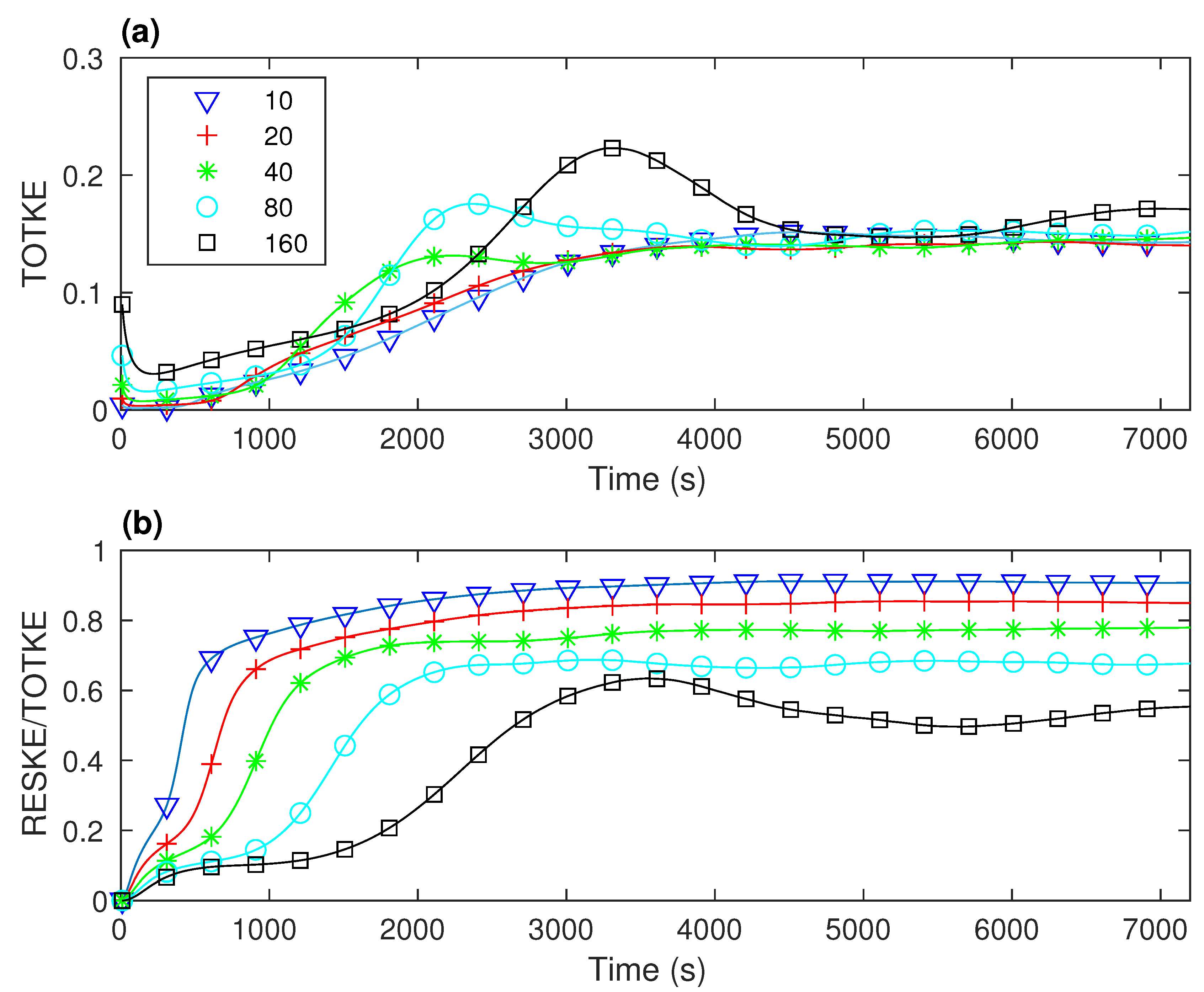
3.1. Turbulent Kinetic Energy

We first consider the domain-mean, turbulent kinetic energy (TKE), $(\rho /2)(\overline{u^{\prime 2}}+\overline{v^{\prime 2}}+\overline{w^{\prime 2}})$. As the resolution is reduced, the resolved turbulent kinetic energy is expected to decrease, but the total TKE (resolved plus sub-filter) should remain the same. This is illustrated with simulation results from CBL1. The TKE time series in Figure 2a show that the simulations with a grid length of 10 m and 20 m produce a monotonic increase (after a slight initial dip) in the total kinetic energy; the values in the two simulations differ slightly up to about 3000 s and then converge. The coarser resolution simulations produce overshoots between around 2000 and 3000 s in the simulation, these becoming increasingly later and more pronounced as the grid length increases. The total kinetic energy in these lower resolution runs converged reasonably well with the higher resolution ones from about 4500 s onwards, albeit with some slow, weak oscillations still persisting at the coarsest resolutions. As discussed in Section 1, previous studies [10,11,12,13,14] suggested that a grid length of 25 m is sufficient for modelling the turbulent CBL. Our results with the 10 and 20 m runs are consistent with that expectation.

Figure 2b shows the resolved TKE as a fraction of the total TKE for each simulation. As expected (e.g., [3,12]), the explicit scale awareness of the Smagorinsky–Lilly approach means that the fraction of resolved TKE increases, and therefore, the amount of sub-filter TKE decreases, with reduced grid spacing. As pointed out by Matheou and Chung [14], Matheou [42], a simple estimate for the scaling of unresolved TKE with grid length $\Delta$ can be obtained under the approximation of a spectral cut-off in the inertial subrange. The estimate of the unresolved TKE, $D(\Delta )$, is then given by integrating the Kolmogorov spectral energy density so that:

$$D(\Delta )\approx {\int }_{k_{\Delta }}^{\infty }C{ϵ}^{2/3}{k}^{-5/3}dk,$$

(11)

where C is the Kolmogorov constant, $ϵ$ is the dissipation rate, k is wavenumber and $k_{\Delta }$ is the cut-off wavenumber corresponding to the grid spacing $\Delta$. The dissipation rate is diagnosed following Section 2 of Brown et al. [40]. The integration yields $D(\Delta )\sim k_{\Delta }^{-2/3}\sim {\Delta }^{2/3}.$ Hence, doubling the grid spacing $\Delta$ should increase the unresolved TKE by a factor of $2^{2/3}\approx 1.6$. Indeed, it is found that the sub-filter energy increases by a factor between $1.5$ and $1.6$ each time the grid spacing is doubled from the 10 m LES run to the 160 m run (

Table 3. Resolved kinetic energy (RESKE), subgrid kinetic energy (SUBKE) and the scaling factor of sub-filter energy with each successive doubling of $\Delta$ for CBL1 simulations with different grid lengths.

	10 m	20 m	40 m	80 m	160 m
RESKE	0.1298	0.1191	0.1144	0.1054	0.0838
SUBKE	0.0132	0.0210	0.0323	0.0496	0.0749
$D(\Delta )$ factor	—	1.592	1.5400	1.5357	1.5084

). Direct inspection of the energy spectra confirms that all simulations produce some $k^{-5/3}$ dependence, over a wider range of scales as the resolution is increased.

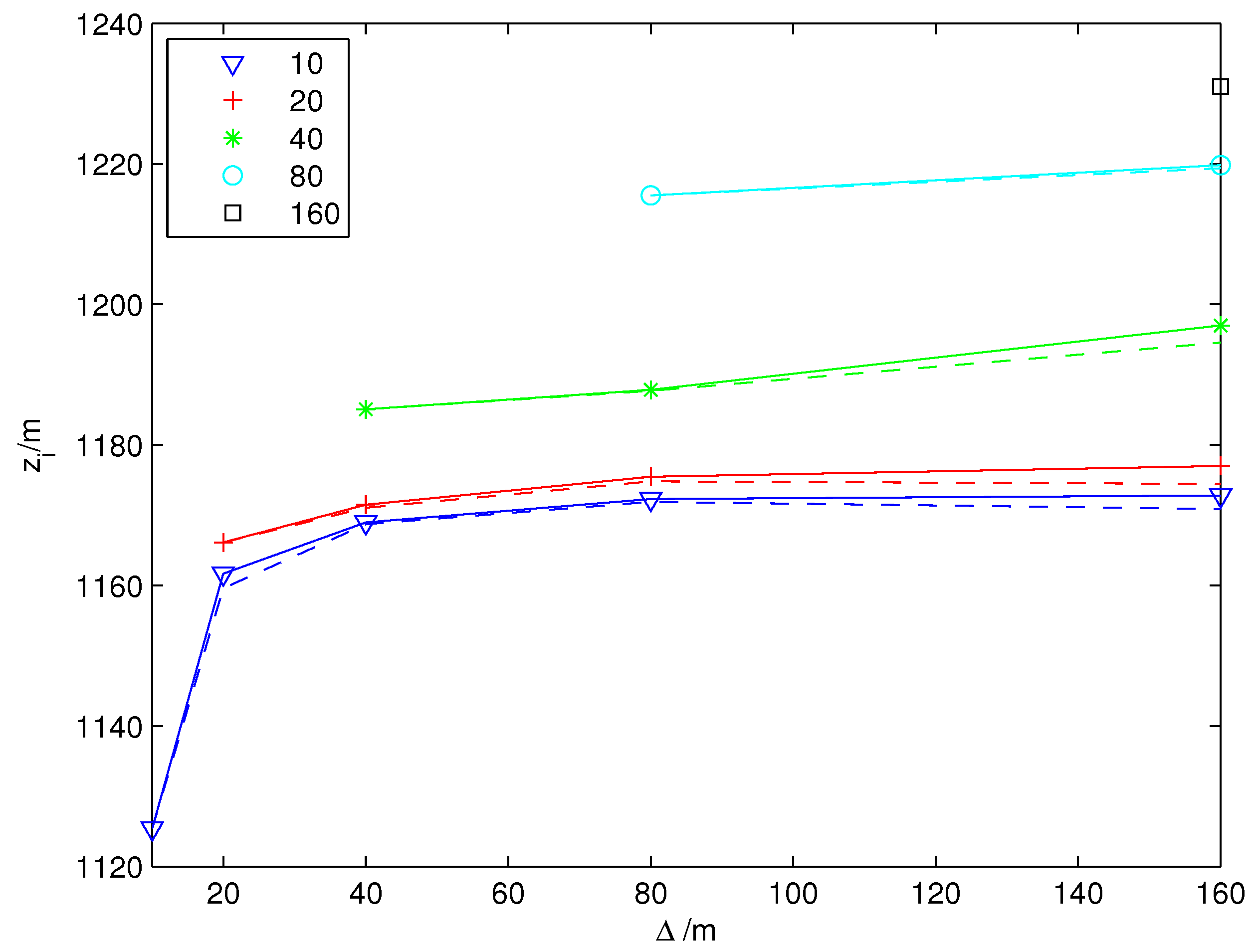
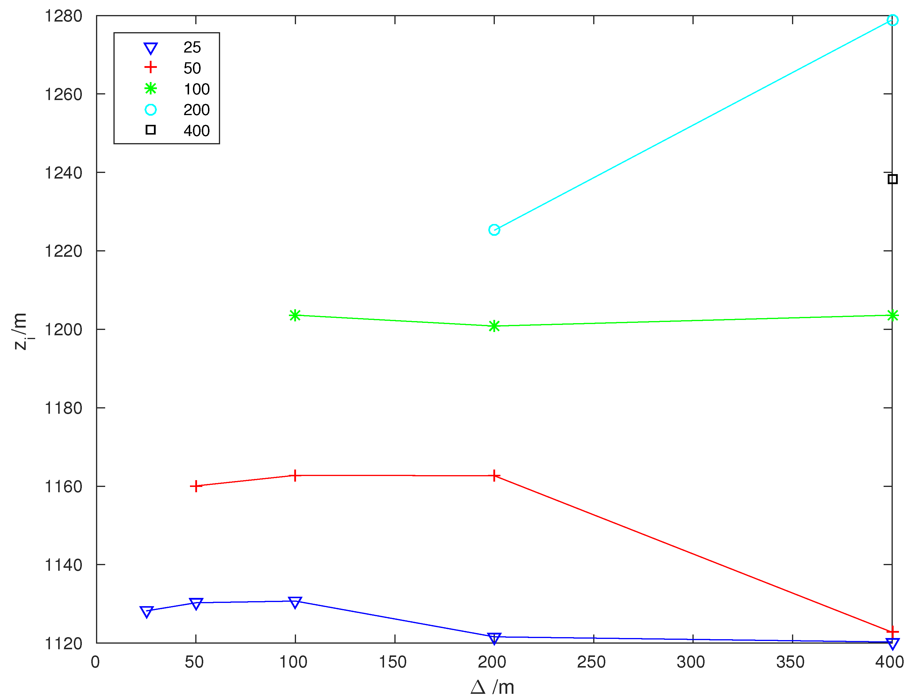
3.2. Boundary Layer Height

The boundary layer (BL) height $z_i$ is calculated using the gradient method of Sullivan et al. [24], which looks for the largest increase in potential temperature with height for each horizontal location. A domain-wide BL height is then obtained by area-averaging the local BL height over all the horizontal grid points. Alternative definitions have been used elsewhere, such as the height of the minimum in the area-averaged heat flux. Sullivan et al. [24] found that the gradient method gives BL heights that are higher than those obtained with the flux method and that are slightly lower than the height reached by the strongest thermals. Using direct numerical simulations of a CBL, Garcia and Mellado [23] found the gradient method to represent the mean vertical extent reached by the penetrating thermals. Our intention is not to compare the relative merits of these different methods for determining the BL height, but rather to compare the BL height thus computed for different grid spacings.

Figure 3 shows the boundary layer height determined 2 h into each simulation from the CBL1 set. The first point on each line denotes the BL height determined from data produced on the native grid of each simulation. As the grid spacing increases, the BL height increases monotonically, ranging from 1130 m at a 10 m grid length to 1229 m at a 160 m grid length. This is consistent with the results of Sullivan and Patton [11], who also found that lower resolutions give higher BL heights. As we investigate later, such results suggest that when lower resolution is used, the thermals may penetrate deeper into the inversion layer. In all of the simulations, the BL height changes slightly over the period of 14 min considered in the analysis of Section 4.2, but by less than 10 m in all cases.

Data from the higher resolution simulations were coarse grained in all three spatial dimensions in order to correspond to each of the various lower resolution grids. Results obtained from computing the BL height using the coarse grained data are also shown in Figure 3. Coarse graining produces a larger BL height in all cases. Both the horizontal and vertical aspects of coarse graining contribute to height increase, although coarse graining in the horizontal (dashed lines) is the dominant aspect. The largest increase results from coarse graining the 10 m data onto the 20 m simulation grid: an increase of about 35 m, or about $4\Delta z$ based on the 8 m vertical grid spacing. The increases produced by coarse graining from or to other grids are much smaller. In all cases, the effect of coarse graining is to produce a BL height that is closer to, but still less than, that computed from data produced natively on that grid.

These results indicate that the differences in the BL height between the different simulations are a robust signal of some differences in the characteristics of the turbulent flow and can only be partially accounted for by the differences in the scale at which the data are considered. For example, the difference in BL height between the 160 m simulation on its native grid and the 10 m simulation coarse grained onto that same grid is 60 m. Since the coarse graining from the 10 to 20 m grid brings the resulting BL heights much closer together (within about 5 m), we also conclude that the 20 m simulation is almost as good as the 10 m one (at least by this measure), with most of the difference being accounted for by a difference in the density of sampling points.

The simulations in set CBL2 include coarser grid spacings of up to 400 m, with a corresponding vertical grid spacing of 160 m. The BL height calculated from these simulations on their native grids also increases as the grid spacing increases (Figure 4). The coarse graining shown on this figure was done in three dimensions. The BL height calculated from the coarse grained data is higher than for the native grid except when a grid spacing of 400 m is used. The BL height for 25 m native resolution coarse grained to 200 m and 400 m is lower than that obtained from the data on the native grid. These results show that the structure of the simulated BL changes as one enters the grey zone.

3.3. Temperature Profile

Figure 5a shows the potential temperature profile obtained from the 25 m grid spacing simulation in set CBL2, as well as from the data coarse grained to 50, 100, 200 and 400 m. The panel represents the expected profile for the different grids. Figure 5b shows the profiles computed from each of the simulations on its native grid. Close to the surface, the temperature increases as the grid spacing increases. Between about $0.1z_i$ and $0.6z_i$, the profiles for the four higher resolution simulations nearly coincide, and all of these simulations are able to produce a clear well-mixed layer [20].

From about $0.6z_i$, the temperature starts to increase and the profiles begin to diverge, and they remain distinct beyond the BL height. Below the BL height, the temperature generally increases more rapidly as the grid spacing increases. Beare [12] and Sullivan and Patton [11] also found that lower resolution simulations gave higher temperatures just below the BL height, and they attributed this to stronger entrainment across the inversion. Similarly, they also found the lower resolution simulations to be associated with a weaker inversion. Similar results are found with CBL1, with higher temperature close to the surface and in the upper boundary layer as the resolution is lowered.

Figure 5b illustrates that the higher resolution simulations cross the $z/z_i=1$ line sooner within their respective inversion layers, which provides a further indication that the thermals are less penetrative within the high resolution simulations. In summary, it appears that overly-penetrative thermals in the lower resolution simulations distort the temperature structure around the BL height somewhat, producing a weaker inversion.

3.4. Heat Flux

Again for CBL2, Figure 6b shows the resolved turbulent heat flux computed from the native 25 m data and also from the data successively coarse grained up to 400 m. It may be noted that similar conclusions were drawn for CBL1; CBL2 is shown here because of the larger range in grid spacing. The flux is normalized by the surface sensible heat flux $Q_{*}$. Figure 6c shows corresponding results using data on the native grid of each simulation. The total flux (Figure 6a) decreases linearly with height and reaches a minimum in the vicinity of the diagnosed BL height, then increases again to a value close to zero. This basic structure is consistent with many previous studies (e.g., [17,22]). The minimum in the total flux occurs a little below $z/z_i=1$, confirming that $z_i$ values determined here from the maximum temperature gradient method are higher than those that would be produced by the minimum flux method. The resolved flux is largest at the highest resolution and decreases as the resolution is decreased.

The layer where the potential temperature flux is negative is known as the entrainment zone. Both the vertical extent of the zone and the magnitude of the peak negative flux have been found to increase with increasing grid length (e.g., [11,12]). The former effect is more apparent in the present simulations, as detailed in

Table 4. The entrainment zone thickness at different grid lengths for the CBL2 simulations, based on the height “Z neg” where the total flux first becomes negative and “Z zero”, above which it is zero. Listed also is the minimum temperature flux, normalized by $Q_{*}$.

	25 m	50 m	100 m	200 m	400 m
Z neg	900	890	890	840	775
Z zero	1210	1200	1260	1240	1150
Thickness	310	310	370	400	375
MinFlux	−0.15	−0.22	−0.21	−0.19	−0.11

. Sullivan and Patton [11] and Beare [12] also analysed the rate of change of the boundary layer height, $d{z}_i/dt$, and concluded that the entrainment rate is higher at lower resolution; this would explain the higher boundary layer temperatures in the lower resolution simulations, as discussed in the previous subsection. To shed further light on the entrainment processes, Sullivan et al. [24], Catalano and Moeng [25] and Park and Baik [19] performed quadrant analyses of the potential temperature flux. We also pursue a quadrant analysis of the resolved potential temperature flux in the next section, but here focused specifically on how the contributions of each quadrant to the total flux depend on grid spacing.

4. The Role of Coherent Structures in Mixing Processes

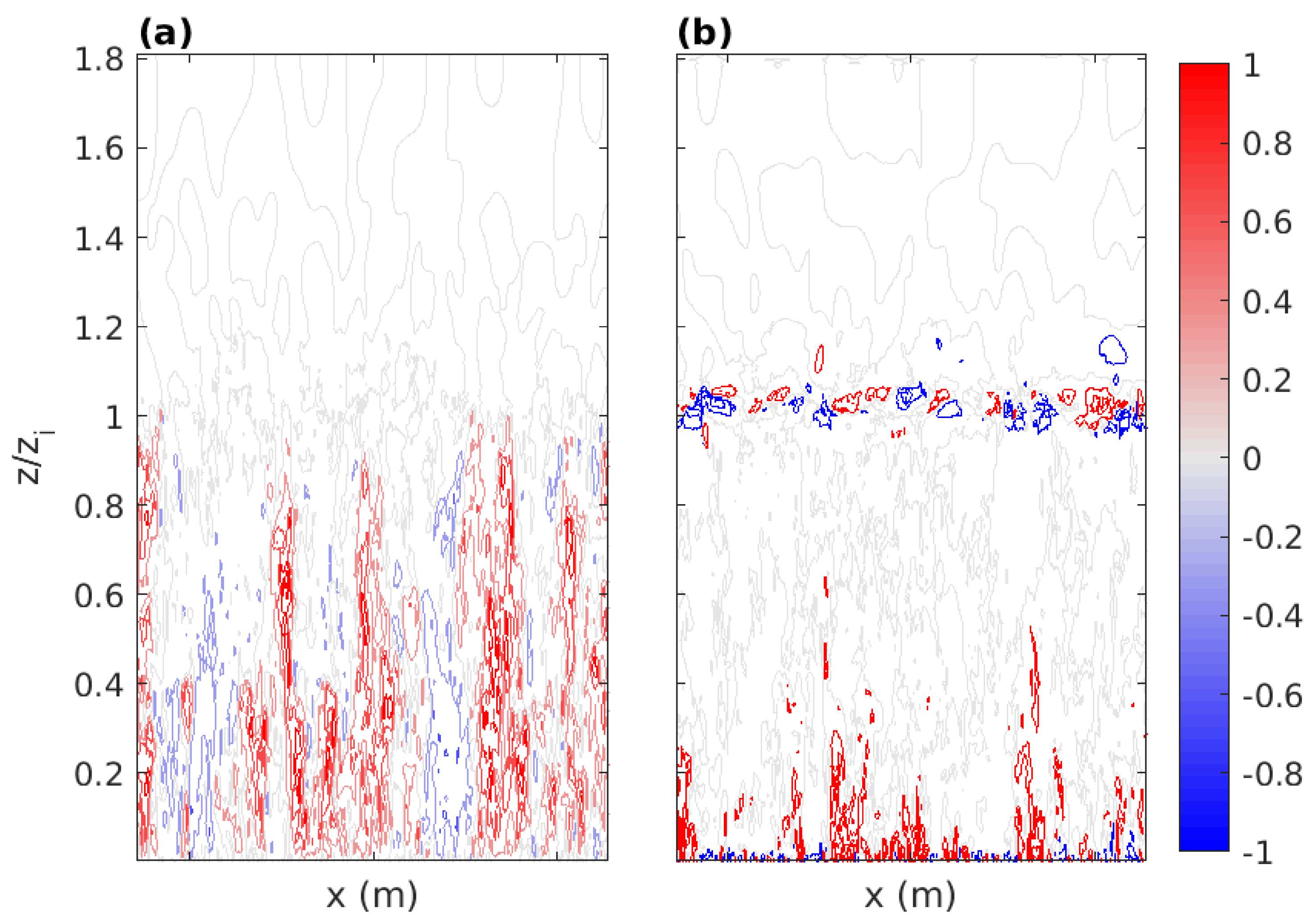
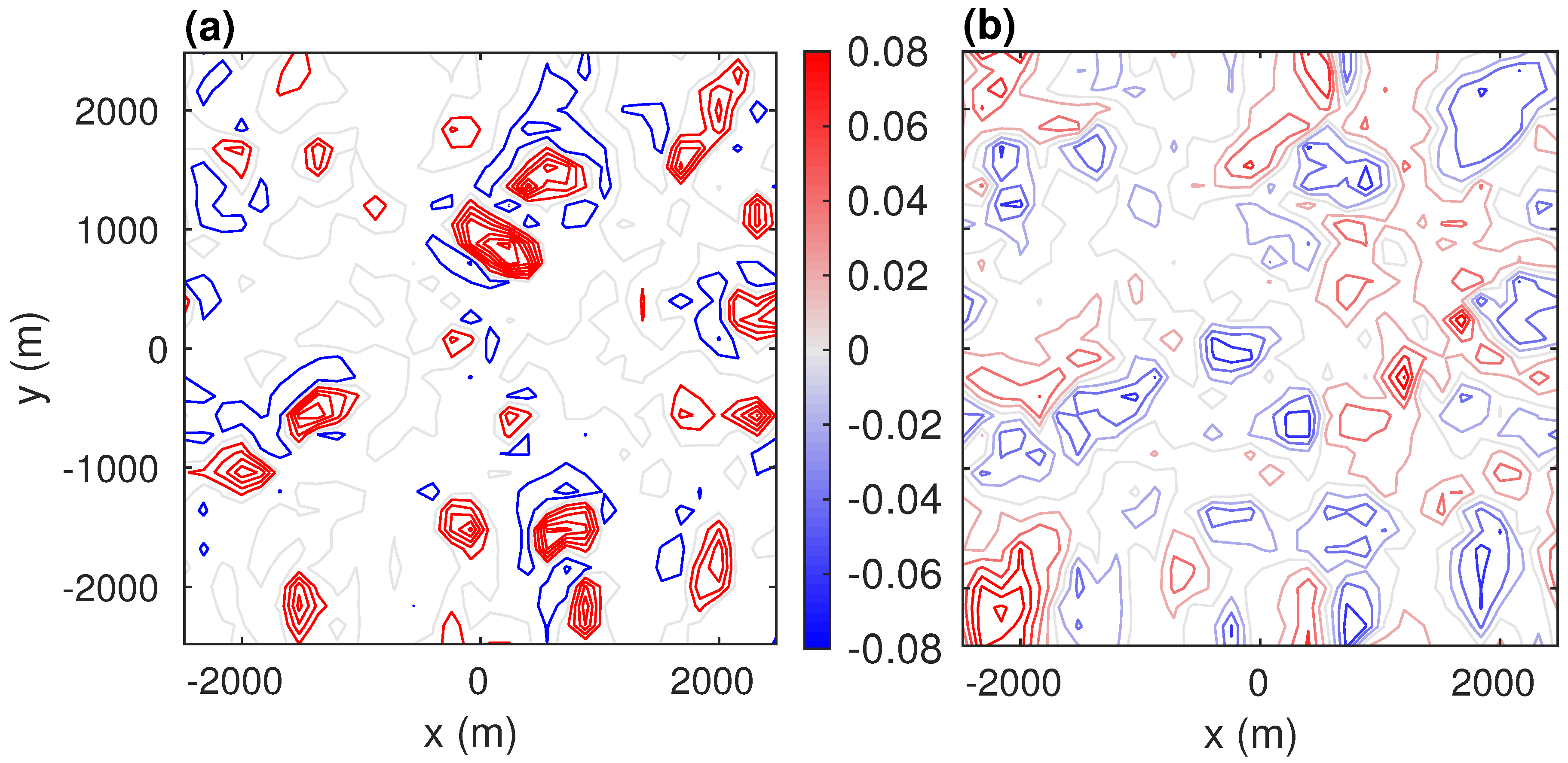
4.1. Flow Visualisation

In order to show the general character of the turbulence, Figure 7 presents a y-z vertical slice of the vertical velocity and the potential temperature perturbations for the $10$ m “truth run” in set CBL1. For the potential temperature, the largest amplitude perturbations are associated with thermals in the lower boundary layer and with overturning motions in the inversion layer. The vertical wind shows that the thermals are vertically coherent structures that extend from the surface all the way to the top of the boundary layer. The tops of the strongest thermals are associated with negative potential temperature perturbations. CBL1 is shown here because it provides the highest resolution; similar results are found with CBL2.

Figure 8 shows corresponding instantaneous x-y cross-sections of vertical velocity and potential temperature perturbations for three different heights. Close to the surface, the regions of upwards motion are relatively disjoint, but at the height of $0.17z_i$ (a,b), these regions start merging together to form thin lines of buoyant upwards motion (i.e., thermals) with broad surrounding regions of descending air. The positive perturbations in both vertical wind and temperature perturbations are well aligned.

At a height of $0.45z_i$ (c,d), around the middle of the boundary layer, the thermals merge further to become more coherent and more isolated features of the flow, surrounded by or surrounding cooler descending air. While the vertical winds in the thermals remain high, the potential temperature perturbations become smaller because of mixing during ascent. Most of the domain is associated with weak negative perturbations of potential temperature. The thermals that are buoyant are more strongly accelerated and have correspondingly larger vertical velocities.

At $0.9z_i$ (e,f), within the entrainment zone, the vertical winds are smaller than at $0.17z_i$ and $0.45z_i.$ Most of the areas of positive vertical velocities correspond to negative potential temperature perturbations. Such regions are the remnants of thermals that have risen all the way from the surface, merging with other thermals as they ascend and accelerate, while becoming colder because of mixing with the environment. Upon arrival at the upper part of the boundary layer, they do not stop rising immediately despite their negative buoyancy. Rather, they decelerate and eventually stop rising, their buoyancy becoming increasingly negative because of the warmer ambient temperatures in the inversion.

As rising air from the thermals reaches the inversion, it moves laterally and then downwards, returning as downdraughts and contributing to the descent of warmer air from the inversion. Such behaviour is shown by the rings of negative vertical wind that surround the thermals, which have been described as downdraughts along the “side wall” of the thermal [20]. These rings of negative wind are generally associated with positive temperature perturbations. Thus, warmer air is drawn deeper into the boundary layer, and this warms the environment as mixing occurs during descent.

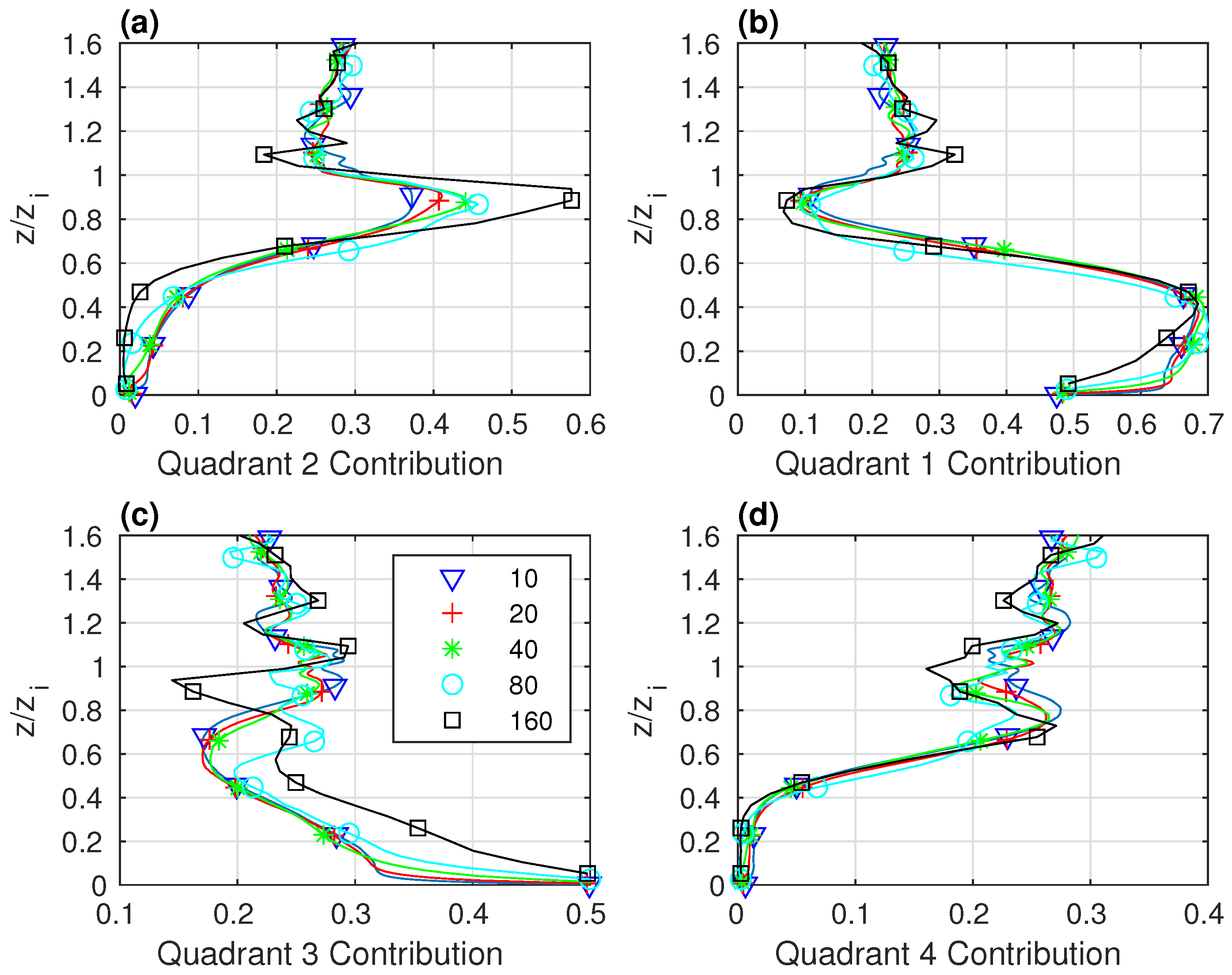
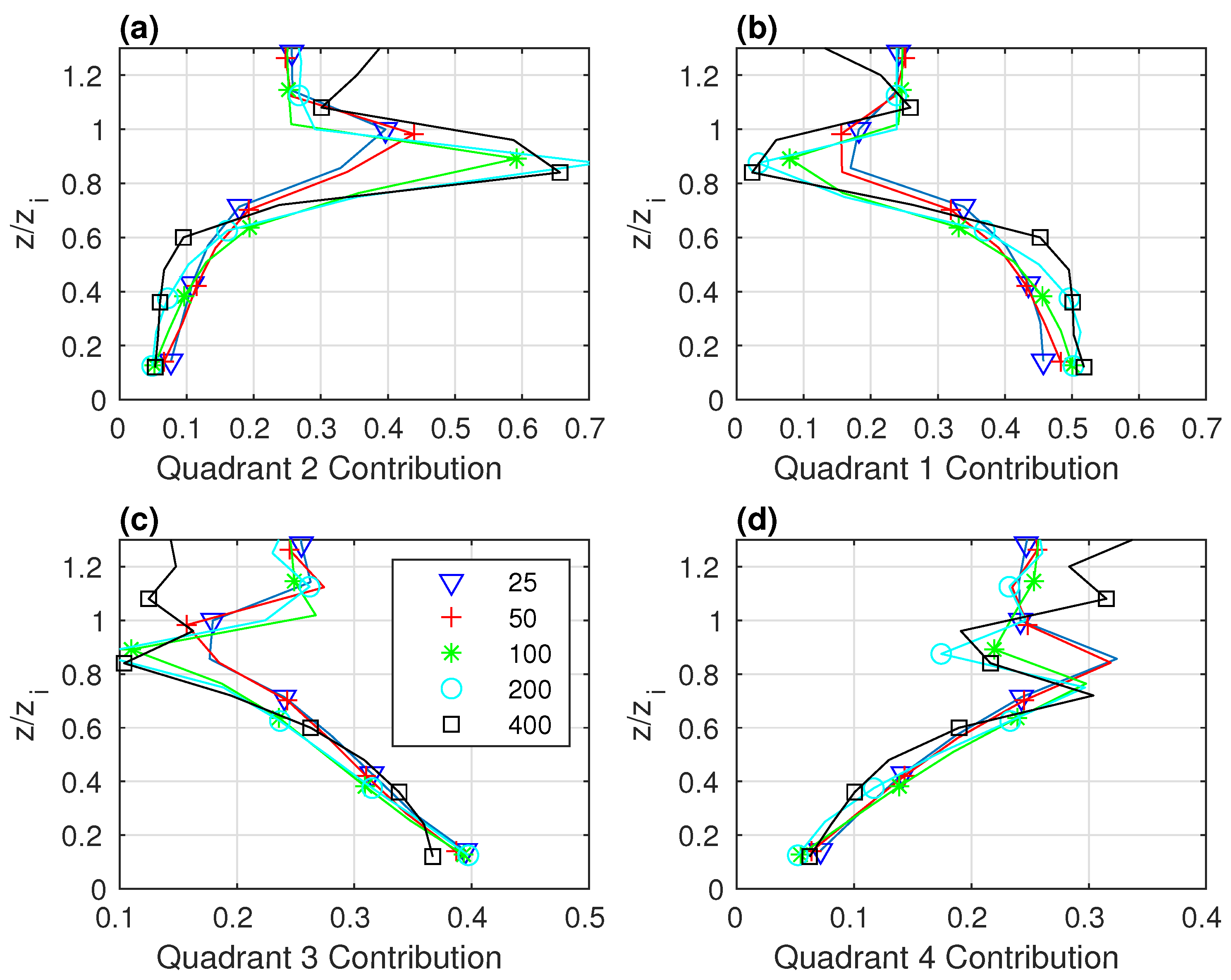
4.2. Quadrant Analysis Based on the “Truth Run”

Further, quantitative, insight into these coherent motions can be gained by means of quadrant analysis. A quadrant analysis of the heat flux is performed by partitioning the combination of vertical velocity (perturbation) and potential temperature perturbation into four quadrants, according to their signs, as follows:

• Q1: $w^{\prime }>0,{\theta }^{\prime }>0$ (warm air rising)
• Q2: $w^{\prime }>0,{\theta }^{\prime }<0$ (cold air rising)
• Q3: $w^{\prime }<0,{\theta }^{\prime }<0$ (cold air descending)
• Q4: $w^{\prime }<0,{\theta }^{\prime }>0$ (warm air descending)

The number of events in each quadrant (i.e., grid-point data combinations satisfying the relevant inequalities), as well as the contribution of each quadrant to the total resolved flux are calculated at every vertical level. The former is normalized by the total number of events and the latter by the total flux at that level in order to produce quantities for which the sum over all quadrants gives a height-independent value of unity as in [43] for example. In this subsection, we discuss the average flux per event, the number of events in each quadrant and the net contribution of each quadrant to the total, all for the 10 m grid length simulation in set CBL1, which we consider as our “truth run”. In the following subsection, we then look at the effects of degrading the resolution.

Figure 9a shows the average resolved flux per event in each quadrant, as well as the average total resolved flux per event. The magnitudes peak around $z_i$. In the immediate vicinity of $z_i$, the contributions from Q2 and Q3 have very similar magnitudes, but opposite signs, and likewise for the contributions from Q1 and Q4. Although the contributions from each of the four quadrants are relatively large here, the similar sizes of the contributions (Figure 9c) and the almost even division of events into each quadrant (Figure 9b) produce an overall cancellation such that the total flux is close to zero. These results within the inversion are similar to those of Sullivan et al. [24] and Park and Baik [19], although the average from Q2 in those previous studies is perhaps slightly larger than in our simulations. The atmospheric profiles in their simulations differ from the present one. It may also be noted that horizontal grid lengths used in Sullivan et al. [24] and Park and Baik [19] are respectively 33 m and 20 m, coarser than for the simulation discussed here. The dependence on grid length will be discussed in the next subsection.

The number of events in each quadrant is shown in Figure 9b. From the surface until just above $z=0.6z_i$, the most common events are for cold descending air (Q3). This is consistent with the snapshots of Figure 8c,d, which illustrate that there are many events in Q3 around the middle of the boundary layer, but with a modest net contribution to the total turbulent flux. The fraction of Q3 events increases quickly very close to the surface, then remains constant at around $0.5$, before it starts to decrease at about $0.35z_i$. The warm ascending (Q1) events are the next most frequent close to the surface, but their number decreases quickly with height such that they are relatively rare within the upper part of the boundary layer, with a minimum at about $0.75z_i$. Q1 events are the least frequent between $z=0.6z_i$ and $z=0.9z_i$. These results have a natural interpretation in terms of thermals that start to rise, mix with the environment, lose buoyancy and ultimately become cold. Air parcels that have become cooler than the environment, but were previously part of a thermal will be assigned to the cold ascending (Q2) quadrant, and so, the relative number of Q2 events increases with height. These negatively buoyant air parcels will decelerate and then begin to descend, thereby contributing to Q3.

The relative contribution of Q1 to the flux increases rapidly close to the surface and then much more slowly through the lower portion of the boundary layer, up to about $0.4z_i.$ Thus, most of the turbulent flux in the lower boundary layer is carried by the thermals, despite the reductions as a function of height to both the average flux associated with each event (Figure 9a) and to their fractional coverage with height (Figure 9b). Although the total heat flux decreases with height in the lower boundary layer, Figure 9 illustrates that this decrease is mainly associated with a reduction in the amplitude of potential temperature perturbations. Those air parcels that remain as thermals (i.e., that are retained within the Q1 quadrant) are accelerated so that the diminishing buoyancy in the Q1 events is partially compensated for by increasing vertical velocity in order to maintain a strong relative contribution to the turbulent heat flux from this quadrant. The decrease in contribution from Q1 at around $0.4z_i$ is coincident with the number of events within Q1 having decreased to less than a quarter.

The contribution from cold descending events (Q3) decreases rapidly with height close to the surface, and more gradually thereafter. In the lower part of the boundary layer, this is due to smaller contributions from individual events, while a reduced number of such events also plays a role in the upper boundary layer.

From about $0.65z_i$ to $0.95z_i$, the most frequent events correspond to warm descending air (Q4). These events indicate entrainment of warm air from the inversion and account for more than a quarter of events down to about $0.5z_i$. These results are consistent with observations, which have reported that the effects of entrainment can be seen down to $0.5z_i$ [20,21]. As the warm air descends, it mixes with the surroundings, becomes colder and starts to make a contribution towards Q3. This interpretation is supported by the shapes of the curves for the number of Q3 and Q4 events between about $0.7z_i$ and the surface (Figure 9b). Although the Q4 events are the most frequent type close to the inversion layer, the largest contribution to the potential temperature flux at these levels comes from the Q2 events, while the relative contribution of the buoyant thermals in Q1 is only around $10\%$. The relatively large contributions from Q2 coincide with the negative values in the total flux. These results are consistent with thermals from the surface that are still rising despite having lost their buoyancy. As the thermals decelerate and terminate, the relative Q2 contribution decreases to about a quarter.

4.3. Resolution-Dependence of Quadrant Contributions to the Heat Flux

Figure 10 shows the relative contributions from each quadrant to the resolved flux for the different CBL1 simulations on their native grids. The main impact of on Q1 occurs close to the surface, where the contributions are reduced for larger grid spacings, particularly for the 160 m simulation. Hence, although there are more buoyant updraught events at coarser resolution, these tend to be considerably weaker and so carry less potential temperature flux overall. However, the most pronounced differences with grid spacing in Figure 10 occur for the Q2 and Q3 quadrants. Up to about $z/z_i$∼0.7, larger grid spacing produces smaller contributions from Q2 and larger contributions from Q3. These changes are at least partially attributable to the numbers of events in those quadrants, but there is also an indication that the flux carried by an individual event in Q3 increases in magnitude for larger grid spacings.

In the entrainment zone, just below the boundary layer height, there is again a substantial resolution dependence in the relative contributions from Q2 and Q3. Specifically, the contribution from Q2 increases for larger grid spacings, whilst that from Q3 decreases. In the previous subsection, we explained that the Q2 events here correspond to thermals that start from the surface as Q1 events, but maintain their ascent even after the buoyancy has changed sign. The number of Q2 events in the upper boundary layer is not very different for different grid spacings, but the associated perturbations are stronger at larger grid spacings, enhancing the resolved flux arising from Q2 in this layer.

Overall, the results of this section imply that at lower resolution, the air parcels associated with buoyant thermals in the lower boundary layer and subsequently with Q2 events in the upper boundary layer undergo less mixing with their environment. As a result, they are able to penetrate further into the inversion layer and produce a somewhat deeper boundary layer (see Section 3.2).

The simulations made with different grid spacings were all coarse grained to 160 m and the quadrant analyses performed on this coarse grained data. At grid spacings from 10 m to 40 m, all the lines fall on top of one another (Figure 11), but some differences are apparent when the grid spacing of 80 m is used. The 160 m grid spacing line is the most distinct and shows the relationships already described above.

Relative contributions from each quadrant in the CBL2 simulations are shown in Figure 12, for comparison with Figure 11. The overall profiles are similar between the two sets of simulations except in the lower boundary layer, in which there is a larger contribution from Q4 (and a correspondingly reduced contribution from Q1) near the surface. The dependence on resolution is qualitatively similar between the two sets, although there is a general impression of a somewhat weaker dependence in the lower boundary layer and a somewhat stronger dependence just below and in the vicinity of the inversion. Quadrant 2 (Figure 11a and Figure 12a) provides a good example of this. The relatively small contributions from Q3 in the coarse resolution simulations above $z/z_i>0.8$ are also a striking feature.

4.4. Resolution Dependence of Structure Length and Time Scales

As discussed in Section 4.1, the convective boundary layer is dominated by buoyancy-driven coherent overturning motions, extending through the depth of the layer. The characteristics of resolved coherent motions are further investigated in this subsection by computing some correlation measures. Figure 13 shows vertical correlations with the mid-layer vertical velocity in the CBL2 simulations. Specifically, we show:

$${\mathrm{VC}}_{\psi \chi }\left(z\right)=\frac{\overline{{\psi }^{\prime }\left(z_{\mathrm{ref}}\right){\chi }^{\prime }\left(z\right)}}{{\overline{{\psi }^{\prime 2}\left(z_{\mathrm{ref}}\right)}}^{1/2}{\overline{{\chi }^{\prime 2}\left(z\right)}}^{1/2}}.$$

(12)

for $\psi =w$ and $z_{\mathrm{ref}}=500$ m. The averaging extends over all horizontal points and snapshots. A decomposition into quadrants is also shown on the figure, and this is constructed by restricting the summation of data values in the numerator of Equation (12) to those times and locations satisfying the relevant quadrant specification at $z=z_{\mathrm{ref}}$. Only results from CBL2 are shown here because of the larger range in spatial resolution.

The large resolved structures are clearly buoyancy-driven, with the correlations being dominated by contributions from the warm ascending quadrant Q1 and, to a lesser extent, the cold descending quadrant Q3. The other quadrants exhibit only weak correlations over a small range of heights between the mid-level vertical velocity and the potential temperature perturbation. The correlation with potential temperature changes sign aloft, since buoyant updraughts in the middle of the boundary layer are associated with cold anomalies aloft as the updraughts overshoot their level of neutral buoyancy. Likewise, cold descending air in the middle of the boundary layer tends to be associated with anomalously warm air within the inversion region, which is again consistent with the interpretation that entrainment across the inversion is related to the presence of the coherent motions within the body of the mixed layer. In order to assess how coherent resolved motions within the boundary layer depend on the grid length, we compare summary measures of correlation for each simulation in set CBL2 to the equivalent measures computed from coarse grained data from the 25 m simulation. As well as the vertical correlations defined in Equation (12), we also construct time correlations defined as:

$${\mathrm{TC}}_{\psi \chi }\left(t\right)=\frac{\overline{{\psi }^{\prime }\left(t_{\mathrm{ref}}\right){\chi }^{\prime }(t_{\mathrm{ref}}+t)}}{\overline{{\psi }^{\prime }\left(t_{\mathrm{ref}}\right){\chi }^{\prime }\left(t_{\mathrm{ref}}\right)}}.$$

(13)

where $t_{\mathrm{ref}}$ denotes a reference time after spin up.

For each correlation function, we can then define a representative length or time scale over which the value of the function has fallen to half of the value at which the constituent fields are colocated and evaluated at the same time. The natural normalizations are provided by the boundary layer height $z_i$ and the eddy turnover time scale $t_{*}=z_i/w_{*}$, respectively. For the vertical correlation function, the criterion may be satisfied by either increasing or decreasing the argument z away from $z_{\mathrm{ref}}$ to yield $z_{+}$ or $z_{-}$, respectively. We define the vertical correlation length scale as being the mean of these values, $(z_{+}+z_{-})/2$.

Figure 14 shows that both the length and time scales increase with increased coarse graining when computed from the results of the 25 m simulation. The same trend is found for simulations performed at increasingly coarse resolution, and it indicates that the dominant resolved eddies become an increasingly dominant aspect of the resolved flow. For example, Figure 14a shows that the correlation length scale for w exceeds $0.4$ at grid spacings of 200 m and 400 m, demonstrating updraughts and downdraughts that retain strong vertical coherence through much of the boundary layer. The buoyancy anomalies also have enhanced vertical coherence on coarser grids, although the coherence in the turbulent heat flux is relatively little changed.

The correlation length scales are somewhat too large in the coarse resolution simulations relative to the coarse grained data, particularly for the buoyancy anomalies. A much more pronounced difference, however, is evident for the time scales in Figure 14b. For example, at 200 m grid spacing, the correlation time scale of the heat flux for the coarse grained data is approximately equal to the eddy turnover time scale, but the simulation with this grid spacing produces a correlation time scale that is $1.6$ times longer. The corresponding factors for the vertical velocity and potential temperature time scales are $1.4$ and $2.9$, respectively. Thus, Figure 14 indicates insufficient time variability in the lower resolution simulations.

5. Discussion

5.1. Temperature in the Boundary Layer

In Section 3.3, we showed that the temperature in the low resolution simulations is warmer close to the surface. The quadrant analysis reveals that low resolution simulations produce more events in the quadrant with warm air that is rising (Q1) and fewer events in the quadrant with cold air that is rising (Q2). Close to the surface, there are steep changes in Q1 and Q3 in the high resolution simulations that are less steep in the lower resolution simulations. Moreover, Q2 events make a larger contribution towards the resolved flux in lower resolution simulations just below the BL height. Taken together, these results provide indications that there is less effective mixing near the surface in the low resolution simulations. We therefore hypothesise that by increasing the mixing, we may see changes in the contributions of the quadrants to more closely match those in the high resolution simulations.

Our results also show that the low resolution simulations are warmer just below the BL height, as in Sullivan and Patton [11] and Beare [12]. These earlier studies attributed the difference to increased entrainment across the inversion within the low resolution simulations, calculated from the rate of change of the BL height. Here, we compute the heating rate due to each quadrant in each simulation directly from the height derivative of the associated resolved potential temperature flux, $\partial <w^{\prime }{\theta }^{\prime }{>}_i/\partial z$. Figure 15 shows these heating rates alongside the total heating rate and the contribution from the sub-filter-scale flux for the CBL1 simulations. In the 10 m grid length “truth” simulation above $0.8z_i$, the heating rate from Q2 roughly cancels that from Q3, while the rate from Q1 roughly cancels that from Q4. Around the BL height $z_i$ itself, the overall heating rate is positive, with contributions from Q2 and Q3 almost cancelling out. Below that level, the largest heating rates are from Q1 and Q4, and immediately below that, it is from Q2 and Q3. As the resolution is coarsened, a mismatch in the heating rates from the different quadrants starts to occur and results in changes to the overall heating rate. The maximum in the heating rate moves from $z_i$ to somewhat lower, and the range of heights just below the BL height associated with heating increases as the resolution coarsens. This will have the effect of eroding the inversion and deepening the boundary layer. The heating rate due to the Q2 quadrant is most notably associated with this change to the overall heating, as seen most clearly in Figure 15d. Indeed, the magnitude of the Q2 contributions increases substantially as the resolution is coarsened, with increased cooling around $0.8z_i$, as well as increased heating around $0.9z_i$ and higher. Snapshots of w and ${\theta }^{\prime }$ are shown in Figure 16 for the 160 m grid length simulation and confirm that there are more Q2 events at low resolution that are strong in the upper part of the boundary layer.

In order to perform low resolution simulations that can better replicate the potential temperature structure and boundary layer height of the highest resolution simulation, it would be necessary either for the contributions of Q1, Q3 and Q4 towards the heating rate in the upper boundary layer to be increased or else for the contributions of Q2 to be decreased. Catalano and Moeng [25] and Park and Baik [19] showed that when a wind shear profile is introduced or is increased, the contributions from other quadrants increase, so that the bias we associate here with Q2 may be less problematic. Overall, the low resolution results are consistent with the hypothesis of insufficient mixing, particularly between the thermals and the surrounding air. The higher boundary layer height in the lower resolution simulations appears to be attributable to cold ascending air that does not lose momentum as quickly as in the high resolution simulations. A related point is that the thermals are too persistent in the lower resolution simulations.

5.2. Increased Mixing

We might anticipate that better results could be obtained by increasing the mixing that takes place in low resolution simulations, so that the contribution from Q2 is reduced below the inversion layer, while the contributions from Q1, Q3 and Q4 may be expected to increase. We tested the hypothesis by repeating some of the lower resolution simulations with increased mixing. The simplest method for doing so is to retain the sub-filter model of Section 2.2, but increase the mixing length $\lambda$. We also experimented by using the stochastic backscatter scheme of Mason and Thomson [34], Weinbrecht and Mason [35] since this has been shown to produce improved simulations of the convective boundary layer in the coarse LES regime, at least for velocity and scalar variances close to the surface. In the next two subsections, we show how the various contributions to the potential temperature flux change when mixing is varied in these ways. To do so, the set CBL1 was augmented with additional runs as described below.

5.2.1. The Effect of Changing the Smagorinsky Constant

Four additional simulations were made with a grid length of 160 m and different values of the mixing length. The mixing length from the original simulations that used a Smagorinsky constant of $0.23$ asymptotes to 37 m away from the surface. In the additional simulations, asymptotic mixing lengths of 17, 27, 47 and 57 m were used. The same domain size and other settings were used as described in Section 2.3.

Figure 17 shows the contribution of each quadrant to the potential temperature flux using different values of the mixing length. As expected, for increased mixing, the contributions of Q1 and Q4 increase in the upper part of the boundary layer, while that of Q2 decreases. The contributions of Q2 with 47 m and 57 m mixing lengths are closer to the LES contributions, which are shown in purple. However, the contributions from Q3 are reduced there. The reduction in Q2 in the middle and upper parts of the boundary layer is very clear, and there is a corresponding change to the boundary layer height, which did decrease somewhat as the mixing increased. A mixing length of 17 m gives a boundary layer height that is 17 m higher than the original simulation using a 37 m mixing length, while a mixing length of 57 m gives a boundary layer height that is 9 m lower.

The robustness of these results was tested by also performing simulations for a grid length of 320 m and with asymptotic mixing lengths of 50, $73.6$ (the case of $c_s=0.23$), 100 and 150 m with a horizontal domain size that is double that used for the other CBL1 simulations. For this configuration, however, changing the value of the mixing length did not change the contribution from Q2 substantially. Thus, it would appear that increased mixing is somewhat helpful in improving simulations with limited resolution for coarse LES, but that this simple remedy is not able to improve grey zone simulations at grid spacings that are more typical of current high resolution NWP.

5.2.2. The Effect of Introducing Stochastic Backscatter

Simulations with stochastic backscatter were performed with grid lengths of both 160 and 320 m, on a domain size that is double that used for the other CBL1 simulations described in Section 3. The same value of $c_s=0.23$ was used for the Smagorinsky constant in each simulation. The resolved kinetic energy increases by just over $40\%$ and $60\%$ in the 160 m and 320 m grid length simulations, respectively, while the total subgrid energy is reduced by a small percentage (

Table 5. Total kinetic energy (TOTE), resolved kinetic energy (RESKE), subgrid kinetic energy (SUBKE) and average boundary layer height ($z_i$) from CBL1 simulations with 160 and 320 m grid lengths with (subscript b) and without (no subscript) backscatter.

	160 m	${160}_{\mathit{b}}$ m	320 m	${320}_{\mathit{b}}$ m
TOTE	0.1542	0.1838	0.1760	0.2146
RESKE	0.0793	0.1113	0.0669	0.1073
SUBKE	0.0750	0.0725	0.1091	0.1074
$z_i$	1267.3	1261.8	1280	1290.7

) when backscatter is used. Backscatter also removes the overshoot problem in the spin-up phase that is found in lower resolution simulations, as discussed in Section 3.1. The spin-up is smoother and more rapid with backscatter included.

Consistent with the expectations for increased mixing between the updraughts and their environment, the contributions of Q1, Q3 and Q4 increase just below the inversion layer when backscatter is used, and likewise, the contribution of Q2 decreases. However, the changes are rather weak. The height of the boundary layer in the 160 m grid length simulation decreases by about $5.5$ m while that of the 320 m grid length simulation increases by just over 10 m (Table 5). This result also suggests that the use of backscatter is not a sufficient remedy within the boundary layer grey zone regime.

6. Conclusions

The MetLEM was used to perform simulations of a convective boundary layer, at horizontal grid lengths ranging from 10 to 400 m, in order to study the effects of reducing the resolution on the coherent resolved motions in a thermally-driven CBL. As in previous studies, we find that a grid length of order 25 m is sufficient to provide an accurate simulation of the convective boundary layer. The boundary layer height increases, and the temperature increases both close to the surface and in the inversion layer, when larger grid spacings are used.

A quadrant analysis shows that the lower part of the boundary layer contains mainly descending cold air events (Q3), followed by ascending warm air events (Q1). A steep decrease with height in the number of Q1 events and a steep increase in the number of Q3 events becomes more gradual as resolution decreases. The Q1 events are associated with thermals and make the largest contribution to the total resolved flux in the lower boundary layer. In the upper part of the boundary layer and just below the inversion layer, there is a large contribution towards the total flux from the Q2 quadrant, associated with decelerating thermals with negative buoyancy. For coarser resolution simulations, the Q2 contributions are found to increase, while the contributions decrease from Q1, Q3 and Q4. Correlation length and time scales for coherent resolved motions increase with larger grid spacings. The time scales in particular are too long in lower resolution simulations relative to the scales that occur in coarse grained data from the high resolution simulation. We calculated heating rates arising from the resolved turbulence in each quadrant and found that the flow in Q2 acts to warm the atmosphere just below and at the boundary layer height and that the strength and depth of this warming increases as the resolution is made coarser. The results therefore suggest that a deeper boundary layer that is warmer just below the BL height is caused mainly by the changes in Q2 rather than by direct changes to the entrainment process.

The results suggest that lower resolution simulations might be improved by increasing the mixing between the decelerating thermals and their environments, in order to reduce the contributions from Q2. We changed the strength of mixing by changing the value of the mixing length in the Smagorinsky scheme. Doing so resulted in a reduction of the contribution of Q2 just below the boundary layer height and an increase in the contributions of Q1 and Q4, as intended. However, the contribution of Q3 at these levels was reduced with the increased mixing, which is an unwanted feature, perhaps implying insufficient penetration of the thermals into the inversion and hence insufficient entrainment. We also performed simulations with and without stochastic backscatter. The introduction of backscatter produced the desired effects in simulations with a 160 m grid length, thereby suggesting that it is desirable to increase mixing in a more targeted way than a simple increase of the mixing length. However, backscatter proved much less effective for a grid length of 320 m.

In summary, our results show that coarser resolution simulations that are still within the LES regime can be improved easily by increasing mixing, either using backscatter or modifying the mixing length. However, the use of backscatter or of changing the mixing length throughout the domain does not seem to provide suitable remedies within the grey zone. A variety of grey zone parameterizations that seek to modify mixing in a more targeted manner [8] are being actively developed and investigated. We believe that analyses such as that presented here, focussed on the properties and behaviour of the dominant resolved eddies as a function of scale, should form an important part of such investigations in order to build confidence that improved results can be produced for sound physical reasons.

References

1. Bauer, P.; Thorpe, A.; Brunet, G. The quiet revolution of numerical weather prediction. Nature 2015, 525, 47–55. [Google Scholar] [CrossRef] [PubMed]
2. Stull, R.B. An Introduction to Boundary Layer Meteorology; Kluwer Academic Publishers: Dordrecht, The Netherlands, 1988; p. 666. [Google Scholar]
3. Honnert, R.; Masson, V.; Couvreux, F. A diagnostic for evaluating the representation of turbulence in atmospheric models at the kilometric scale. J. Atmos. Sci. 2011, 68, 3112–3131. [Google Scholar] [CrossRef]
4. Hanley, K.E.; Plant, R.S.; Stein, T.H.M.; Hogan, R.J.; Lean, H.W.; Halliwell, C.; Clark, P.A. Mixing length controls on high resolution simulations of convective storms. Q. J. R. Meteorol. Soc. 2015, 141, 272–284. [Google Scholar] [CrossRef]
5. Thurston, W.; Fawcett, R.J.B.; Tory, K.J.; Kepert, J.D. Simulating boundary layer rolls with a numerical weather prediction model. Q. J. R. Meteorol. Soc. 2016, 142, 211–223. [Google Scholar] [CrossRef]
6. Doubrawa, P.; Muñoz-Esparza, D. Simulating Real Atmospheric Boundary Layers at Gray-Zone Resolutions: How Do Currently Available Turbulence Parameterizations Perform? Atmosphere 2020, 11, 345. [Google Scholar] [CrossRef] [Green Version]
7. Wyngaard, J.C. Toward numerical modeling in the “terra incognita”. J. Atmos. Sci. 2004, 61, 1816–1826. [Google Scholar] [CrossRef]
8. Honnert, R.; Efstathiou, G.A.; Beare, R.J.; Ito, J.; Lock, A.; Neggers, R.; Plant, R.S.; Shin, H.H.; Tomassini, L.; Zhou, B. The Atmospheric Boundary Layer and the “Gray Zone” of Turbulence: A critical review. J. Geophys. Res. Atmos. 2020, 125, 1. [Google Scholar] [CrossRef]
9. Stoll, R.; Gibbs, J.A.; Salesky, S.T.; Anderson, W.; Calaf, M. Large-Eddy Simulation of the Atmospheric Boundary Layer. Bound. Layer Meteorol. 2020. [Google Scholar] [CrossRef]
10. Wurps, W.; Steinfeld, G.; Heinz, S. Grid-Resolution Requirements for Large-Eddy Simulations of the Atmospheric Boundary Layer. Bound. Layer Meteorol. 2020, 175, 179–201. [Google Scholar] [CrossRef] [Green Version]
11. Sullivan, P.P.; Patton, E.G. The effect of mesh resolution on convective boundary layer statistics and structures generated by Large-Eddy Simulation. J. Atmos. Sci. 2011, 68, 2395–2415. [Google Scholar] [CrossRef]
12. Beare, R.J. A length scale defining partially-resolved boundary layer turbulence simulations. Bound. Layer Meteorol. 2014, 151, 39–55. [Google Scholar] [CrossRef] [Green Version]
13. Park, S.B.; Baik, J.J.; Han, B.S. Characteristics of Decaying Convective Boundary Layers Revealed by Large-Eddy Simulations. Atmosphere 2020, 11, 434. [Google Scholar] [CrossRef] [Green Version]
14. Matheou, G.; Chung, D. Large-Eddy Simulation of Stratified Turbulence. Part II: Application of the Stretched-Vortex Model to the Atmospheric Boundary Layer. J. Atmos. Sci. 2014, 71, 4439–4460. [Google Scholar] [CrossRef]
15. Matheou, G.; Chung, D.; Nuijens, L.; Stevens, B.; Teixeira, J. On the Fidelity of Large-Eddy Simulation of Shallow Precipitating Cumulus Convection. Mon. Weather Rev. 2011, 139, 2918–2939. [Google Scholar] [CrossRef]
16. Moeng, C.H.; Sullivan, S.S. A comparison of shear- and buoyancy-driven planetary boundary layer flows. J. Atmos. Sci. 1994, 51, 999–1022. [Google Scholar] [CrossRef] [Green Version]
17. Khanna, S.; Brasseur, J.G. Three-dimensional buoyancy- and shear-induced local structure of the atmospheric boundary layer. J. Atmos. Sci. 1998, 55, 710–743. [Google Scholar] [CrossRef]
18. Pino, D.; Vila-Guerau de Arellano, J.; Duynkerke, P.G. The contribution of shear to the evolution of a convective boundary layer. J. Atmos. Sci. 2003, 60, 1913–1926. [Google Scholar] [CrossRef] [Green Version]
19. Park, S.B.; Baik, J.J. Large-Eddy Simulations of convective boundary layers over flat and urbanlike surfaces. J. Atmos. Sci. 2014, 71, 1880–1892. [Google Scholar] [CrossRef]
20. Kaimal, J.C.; Wyngaard, J.C.; Haugen, D.A.; Coté, O.R.; Izumi, Y.; Caughey, S.J.; Readings, C.J. Turbulence structure in the convective boundary layer. J. Atmos. Sci. 1976, 33, 2152–2169. [Google Scholar] [CrossRef] [Green Version]
21. Caughey, S.J.; Palmer, S.G. Some aspects of turbulence structure through the depth of the convective boundary layer. Q. J. R. Meteorol. Soc. 1979, 105, 811–827. [Google Scholar] [CrossRef]
22. Moeng, C.H. A Large-Eddy-Simulation model for the study of planetary boundary layer turbulence. J. Atmos. Sci. 1984, 41, 2052–2062. [Google Scholar] [CrossRef]
23. Garcia, J.R.; Mellado, J.P. The two-layer structure of the entrainment zone in the convective boundary layer. J. Atmos. Sci. 2014, 71, 1935–1955. [Google Scholar] [CrossRef] [Green Version]
24. Sullivan, P.P.; Moeng, C.H.; Stevens, B.; Lenschow, D.H.; Mayor, S.D. Structure of the entrainment zone capping the convective atmospheric boundary layer. J. Atmos. Sci. 1998, 55, 3042–3064. [Google Scholar] [CrossRef] [Green Version]
25. Catalano, F.; Moeng, C.H. Large-Eddy Simulation of the daytime boundary layer in an idealized valley using the Weather Research and Forecasting numerical model. Bound. Layer Meteorol. 2010, 137, 49–75. [Google Scholar] [CrossRef] [Green Version]
26. Efstathiou, G.A.; Plant, R.S.; Bopape, M.J.M. Simulation of an Evolving Convective Boundary Layer Using a Scale-Dependent Dynamic Smagorinsky Model at Near-Gray-Zone Resolutions. J. Appl. Meteorol. Clim. 2018, 57, 2197–2214. [Google Scholar] [CrossRef]
27. Boutle, I.A.; Eyre, J.E.J.; Lock, A.P. Seamless Stratocumulus Simulation across Turbulent Gray Zone. Mon. Weather Rev. 2014, 142, 1655–1668. [Google Scholar] [CrossRef]
28. Shin, H.H.; Hong, S. Representation of the subgrid-scale turbulent transport in convective boundary layers at grey zone resolutions. Mon. Weather Rev. 2015, 142, 250–271. [Google Scholar] [CrossRef]
29. Bou-Zeid, E.; Meneveau, C.; Parlange, M. A scale-dependent Lagrangian dynamic model for large eddy simulation of complex turbulent flows. Phys. Fluids 2005, 17, 025105. [Google Scholar] [CrossRef] [Green Version]
30. Efstathiou, G.; Beare, R.; Osborne, S.; Lock, A. Grey zone simulations of the morning convective boundary layer development. J. Geophys. Res. Atmos. 2016, 121. [Google Scholar] [CrossRef] [Green Version]
31. Mason, P.J. Large-eddy simulation: A critical review of the technique. Quart. J. R. Meteorol. Soc. 1994, 120, 1–26. [Google Scholar] [CrossRef]
32. Smagorinsky, J. General circulation experiments with the primitive equations. Mon. Weather Rev. 1963, 91, 99–164. [Google Scholar] [CrossRef]
33. Lilly, D.K. On the computational stability of numerical solutions of time-dependent non-linear geophysical fluid dynamics problems. Mon. Weather Rev. 1965, 93, 11–25. [Google Scholar] [CrossRef]
34. Mason, P.J.; Thomson, D.J. Stochastic backscatter in large eddy simulations of boundary layers. J. Fluid Mech. 1992, 242, 51–78. [Google Scholar] [CrossRef]
35. Weinbrecht, S.; Mason, P.J. Stochastic backscatter for cloud-resolving models. Part I: Implementation and testing in a dry convective boundary layer. J. Atmos. Sci. 2008, 65, 123–139. [Google Scholar] [CrossRef]
36. Germano, M.; Piomelli, U.; Moin, P.; Cabot, W.H. A dynamic subgrid-scale eddy viscosity model. Phys. Fluids A 1991, 3, 1760–1765. [Google Scholar] [CrossRef] [Green Version]
37. Meneveau, C.; Katz, J. Scale-invariance and turbulence models for large eddy simulation. Annu. Rev. Fluid Mech. 2000, 32, 1–32. [Google Scholar] [CrossRef]
38. Shutts, G.J.; Gray, M.E.B. A numerical modelling study of the geostrophic adjustment process following deep convection. Quart. J. R. Meteorol. Soc. 1994, 120, 1145–1178. [Google Scholar] [CrossRef]
39. Piacsek, S.A.; Williams, G.P. Conservation properties of convection difference schemes. J. Comput. Phys. 1970, 6, 392–405. [Google Scholar] [CrossRef]
40. Brown, A.R.; Derbyshire, S.H.; Mason, P.J. Large-eddy simulation of stable atmospheric boundary layers with a revised stochastic subgrid model. Quart. J. R. Meteorol. Soc. 1994, 120, 1485–1512. [Google Scholar] [CrossRef]
41. Lilly, D.K. On the Application of the Eddy Viscosity Concept in the Inertial Sub-Range of Turbulence; Technical Report 123; National Centre for Atmospheric Research: Boulder, CO, USA, 1966. [Google Scholar]
42. Matheou, G. Numerical discretization and subgrid-scale model effects on large eddy simulations of a stable boundary layer. Quart. J. R. Meteorol. Soc. 2016, 142, 3050–3062. [Google Scholar] [CrossRef]
43. Coceal, O.; Dobre, A.; Thomas, T.G.; Belcher, S.E. Structure of turbulent flow over regular arrays of cubical roughness. J. Fluid Mech. 2007, 598, 375–409. [Google Scholar] [CrossRef] [Green Version]
Figure 1. Initial potential temperature profiles for Convective Boundary Layer 1 (CBL1) (blue) and CBL2 (black).
Atmosphere 11 00986 g001
Figure 2. Time series of (a) total (resolved plus sub-filter) kinetic energy (TOTKE) in m 2 s 2 and (b) the ratio of resolved kinetic energy (RESKE) to total kinetic energy, for CBL1 simulations. Each line is for a simulation with a different grid length, the values in m being indicated in the inset.
Atmosphere 11 00986 g002
Figure 3. Boundary layer height diagnosed from each CBL1 simulation plotted at its native grid length and also when computed after coarse graining of the data onto other grids. The solid lines indicate coarse graining in all three directions, whereas the dashed lines are for coarse graining in the horizontal only.
Atmosphere 11 00986 g003
Figure 4. Boundary layer height diagnosed from each CBL2 simulation plotted at its native grid length and also when computed after coarse graining of the data onto other grids. The lines indicate coarse graining in all three directions.
Atmosphere 11 00986 g004
Figure 5. Domain-averaged potential temperature profiles from CBL2 runs (a) for a 25 m grid length and coarse grained to other grids and (b) at different native grid spacings. Each line is for a different coarse graining scale (a) or for a simulation with a different grid length (b), the values in m being indicated in the inset.
Atmosphere 11 00986 g005
Figure 6. Domain-averaged profiles from CBL2 runs (a) for total temperature flux at different native grid spacings and resolved temperature flux (b) for a 25 m grid length and coarse grained to other grids and (c) at different native grid spacings. Fluxes are normalized by the surface value ( Q * ) and shown as a function of the normalized height. Each line is for a different coarse graining scale (b) or for a simulation with a different grid length (c), the values in m being indicated in the inset.
Atmosphere 11 00986 g006
Figure 7. Vertical cross-sections of (a) vertical velocity and (b) potential temperature perturbation for the 10 m grid length “truth run” of CBL1. The range of values that provides a normalization factor for the colour bar in (a) is 1.5 to 1.5 ms 1 and in (b) is 0.1 to 0.1 K.
Atmosphere 11 00986 g007
Figure 8. Horizontal cross-sections of (a,c,e) vertical velocity and (b,d,f) perturbation potential temperatures θ from the 10 m grid length “truth run” of CBL1, at heights of (a,b) 192 m/ 0.17 z i , (c,d) 512 m/ 0.45 z i and (e,f) 1024 m / 0.9 z i . The range of values that provides a normalization factor for the colour bar in (a) and (c) is 1.5 to 1.5 ms 1 , in (e) is 0.08 to 0.08 ms 1 , while that in (b,d,f) is 0.08 to 0.08 K.
Atmosphere 11 00986 g008
Figure 9. Quadrant analysis of the resolved potential temperature flux for the CBL1 “truth run” with a horizontal grid length of 10 m. (a) Average flux per event in each quadrant, normalized by the total potential temperature flux at the surface. Results are shown for Quadrants 1 (red up), 2 (blue up), 3 (blue down) and 4 (red down) and for the total resolved flux (black squares). (b) Number of events in each quadrant, normalized by the total for all quadrants. (c) Relative fractional contributions of the fluxes in each quadrant, computed as | w θ i | / i | w θ i | .
Atmosphere 11 00986 g009
Figure 10. Effect of grid spacing on the partitioning of the resolved potential temperature flux into different quadrants for the CBL1 runs. Relative contributions of the flux in each quadrant, computed as | w θ i | / i | w θ i | , are shown for (a) Quadrant 2, (b) Quadrant 1, (c) Quadrant 3 and (d) Quadrant 4. Each line is for a simulation with a different grid length, the values in m being indicated in the inset.
Atmosphere 11 00986 g010
Figure 11. Effect of coarse graining data from the CBL1 simulations to the 160 m grid on the partitioning of the resolved potential temperature flux into different quadrants. Relative contributions of the flux in each quadrant, computed as | w θ i | / i | w θ i | , are shown for (a) Quadrant 2, (b) Quadrant 1, (c) Quadrant 3 and (d) Quadrant 4. Each line is for a simulation with a different grid length, the values in m being indicated in the inset.
Atmosphere 11 00986 g011
Figure 12. Effect of coarse graining data from the CBL2 simulations to the 400 m grid on the partitioning of the resolved potential temperature flux into different quadrants. Relative contributions of the flux in each quadrant, computed as | w θ i | / i | w θ i | , are shown for (a) Quadrant 2, (b) Quadrant 1, (c) Quadrant 3 and (d) Quadrant 4. Each line is for a simulation with a different grid length, the values in m being indicated in the inset.
Atmosphere 11 00986 g012
Figure 13. The vertical correlation of the 500 m vertical velocity w in the CBL2 25 m simulation with (a) χ = w and (b) χ = θ , as defined in Equation (12). The decomposition of the correlation into contributions from each quadrant is also shown.
Atmosphere 11 00986 g013
Figure 14. The correlation (a) length scales and (b) time scales for correlation functions evaluated at 500 m. The scales for ψ = χ = w are shown in red, for ψ = χ = θ in blue and for ψ = w , χ = θ in green. Scales obtained from the CBL2 simulations with different grid lengths are plotted with solid lines and asterisks against the grid length. Scales obtained after coarse graining the results of the 25 m simulation are plotted with plus symbols and dotted lines.
Atmosphere 11 00986 g014aAtmosphere 11 00986 g014b
Figure 15. Contributions to the rate of change of potential temperature (Ks 1 ) in the CBL1 simulations with grid lengths of (a) 10 m, (b) 40 m, (c) 80 m and (d) 160 m. The contributions due to resolved turbulent fluxes in each of the quadrants are shown, as well as the contributions from all resolved fluxes and that from the sub-filter flux. The symbols and line styles used for each contribution are indicated on the inset to Panel (d).
Atmosphere 11 00986 g015
Figure 16. Horizontal cross-sections of (a) the vertical velocity w and (b) perturbation potential temperatures θ from the CBL1 run with grid length 160 m, at a height of 1024 m ( 0.83 z i ). The colour bar extends from 0.08 to 0.08 ms 1 in (a) and from 0.08 to 0.08 K in (b).
Atmosphere 11 00986 g016
Figure 17. Effect of mixing length on the partitioning of the resolved potential temperature flux into different quadrants for CBL1 runs with 160 m grid spacing. Relative contributions of the flux in each quadrant, computed as | w θ i | / i | w θ i | , are shown for (a) Quadrant 2, (b) Quadrant 1, (c) Quadrant 3 and (d) Quadrant 4. Each line is for a simulation with a different value of the asymptotic mixing length, the values in m being indicated in the inset. LES results from the 10 m simulation are also shown.
Atmosphere 11 00986 g017