An Assessment of Observed and Simulated Temperature Variability in Sierra de Guadarrama

Abstract
1. Introduction
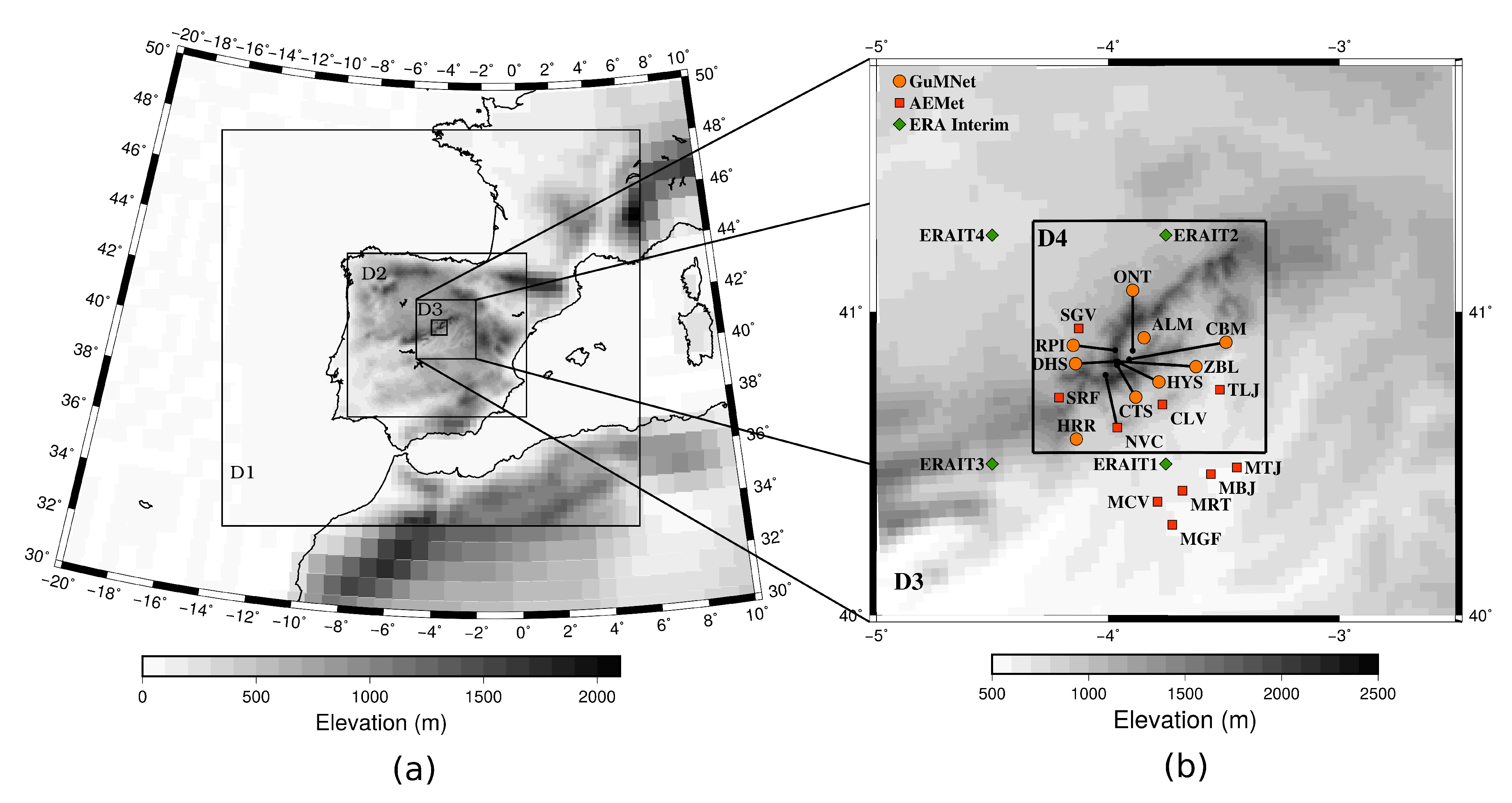
2. Data
2.1. WRF Model Simulations

2.2. ERA Interim Reanalysis Data
2.3. Observations
3. Methodology
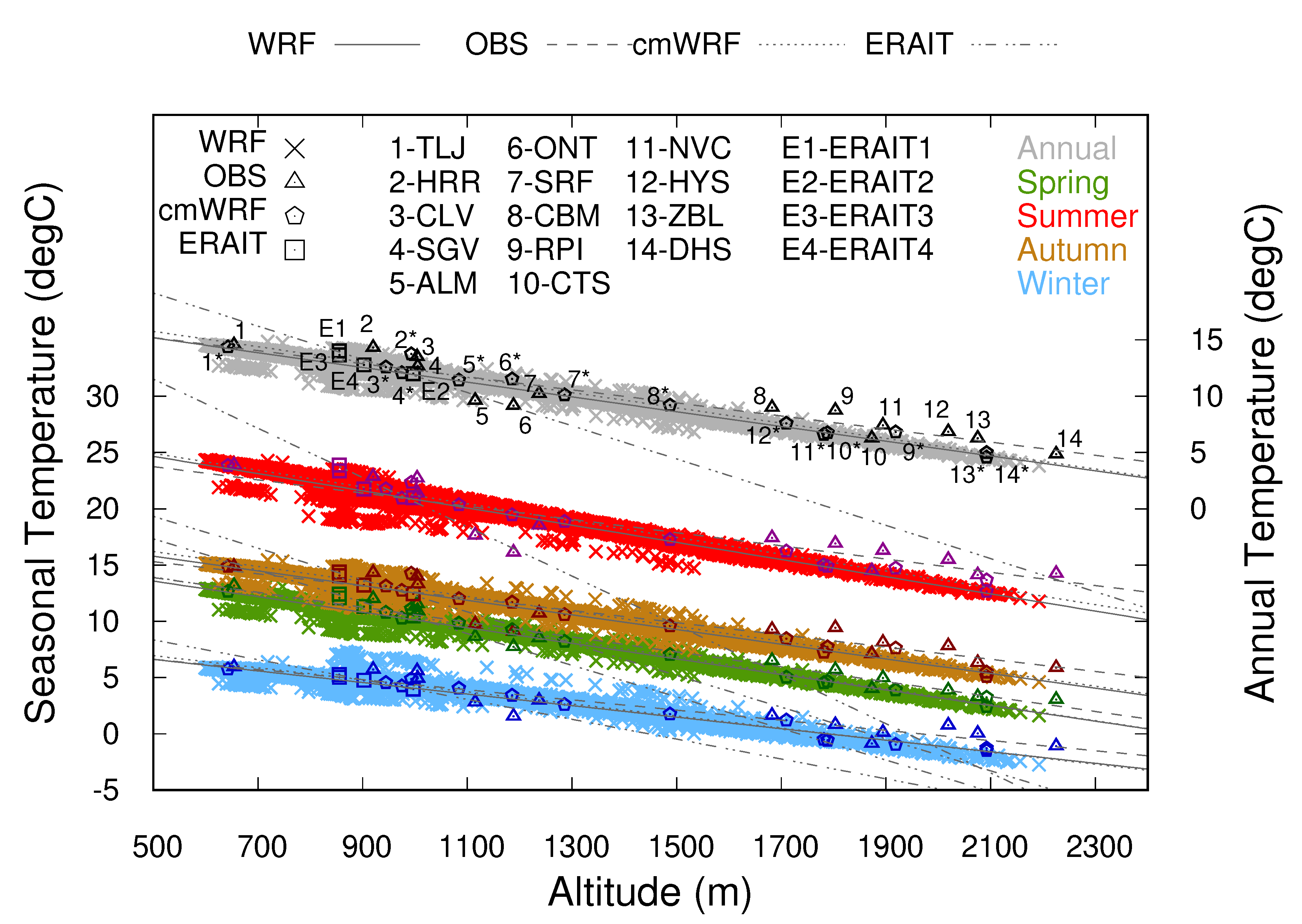
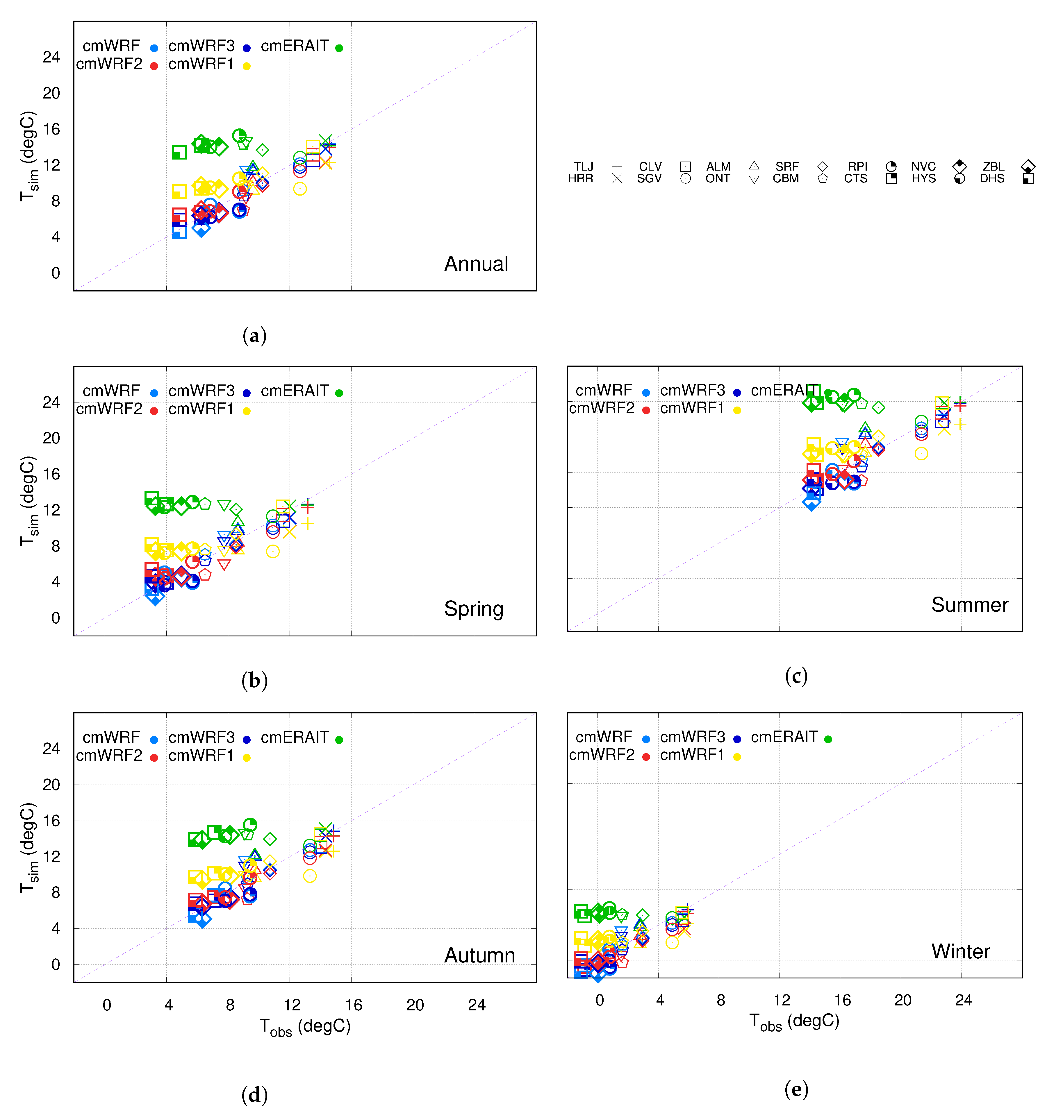
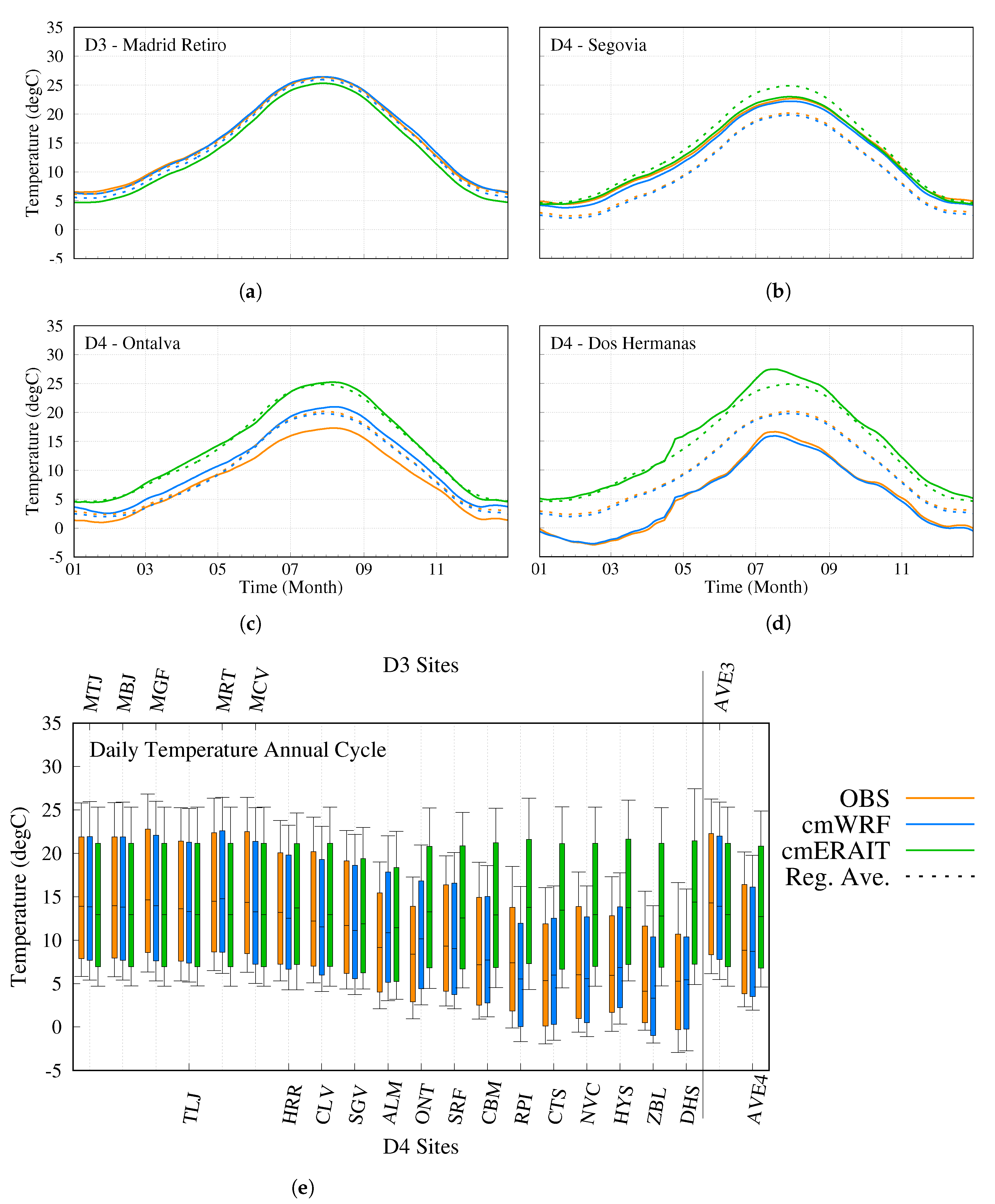
4. Results
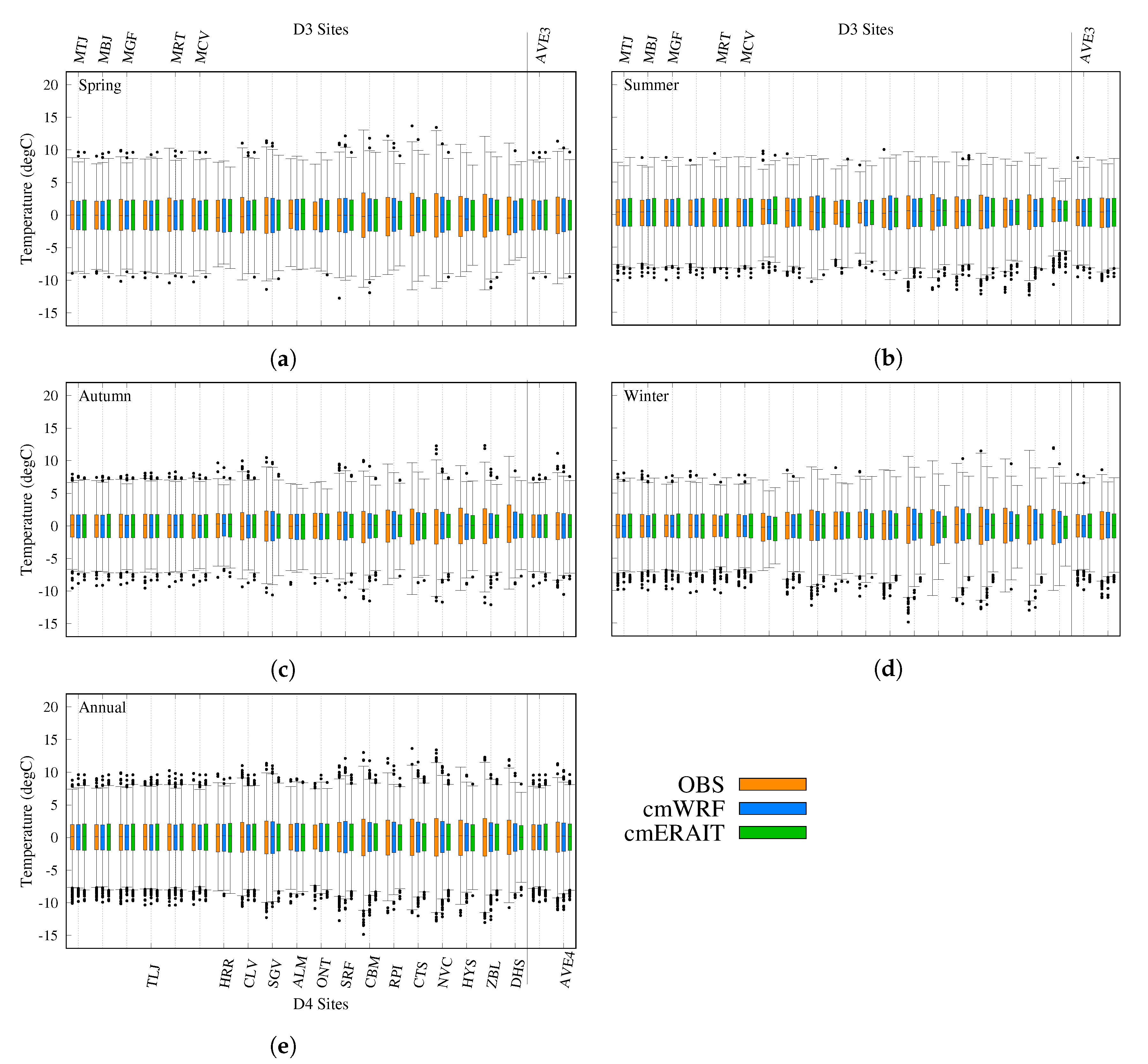
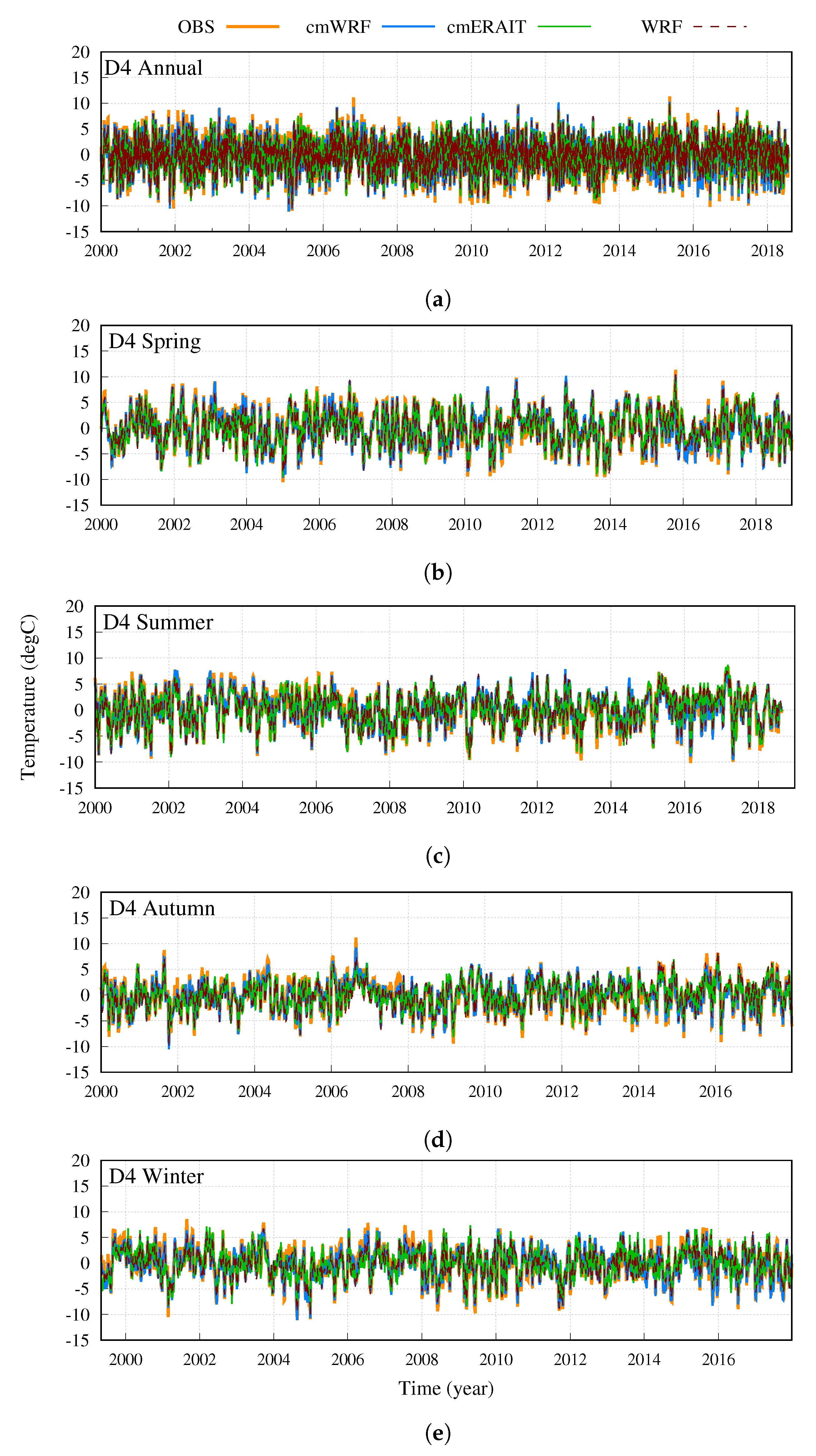
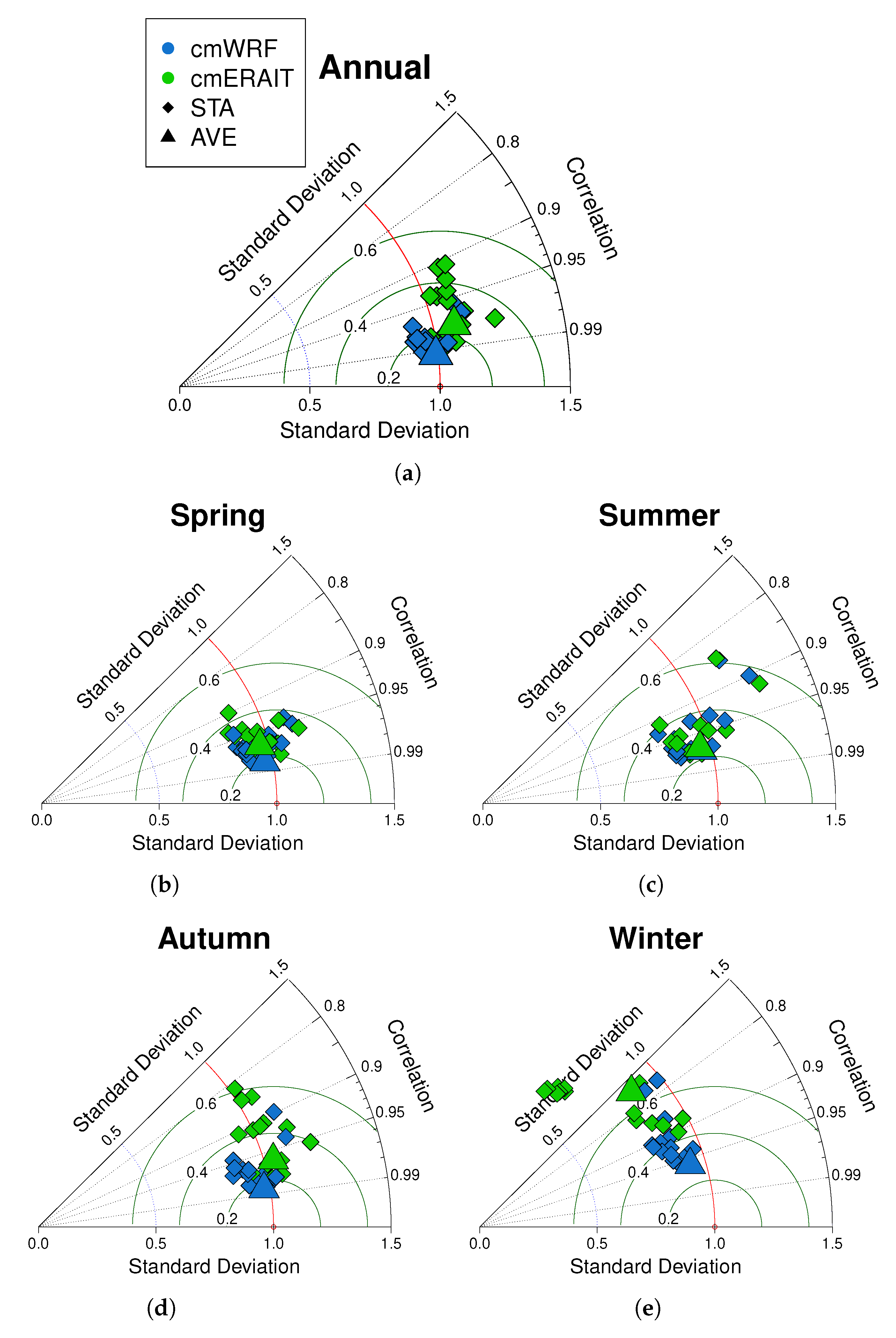
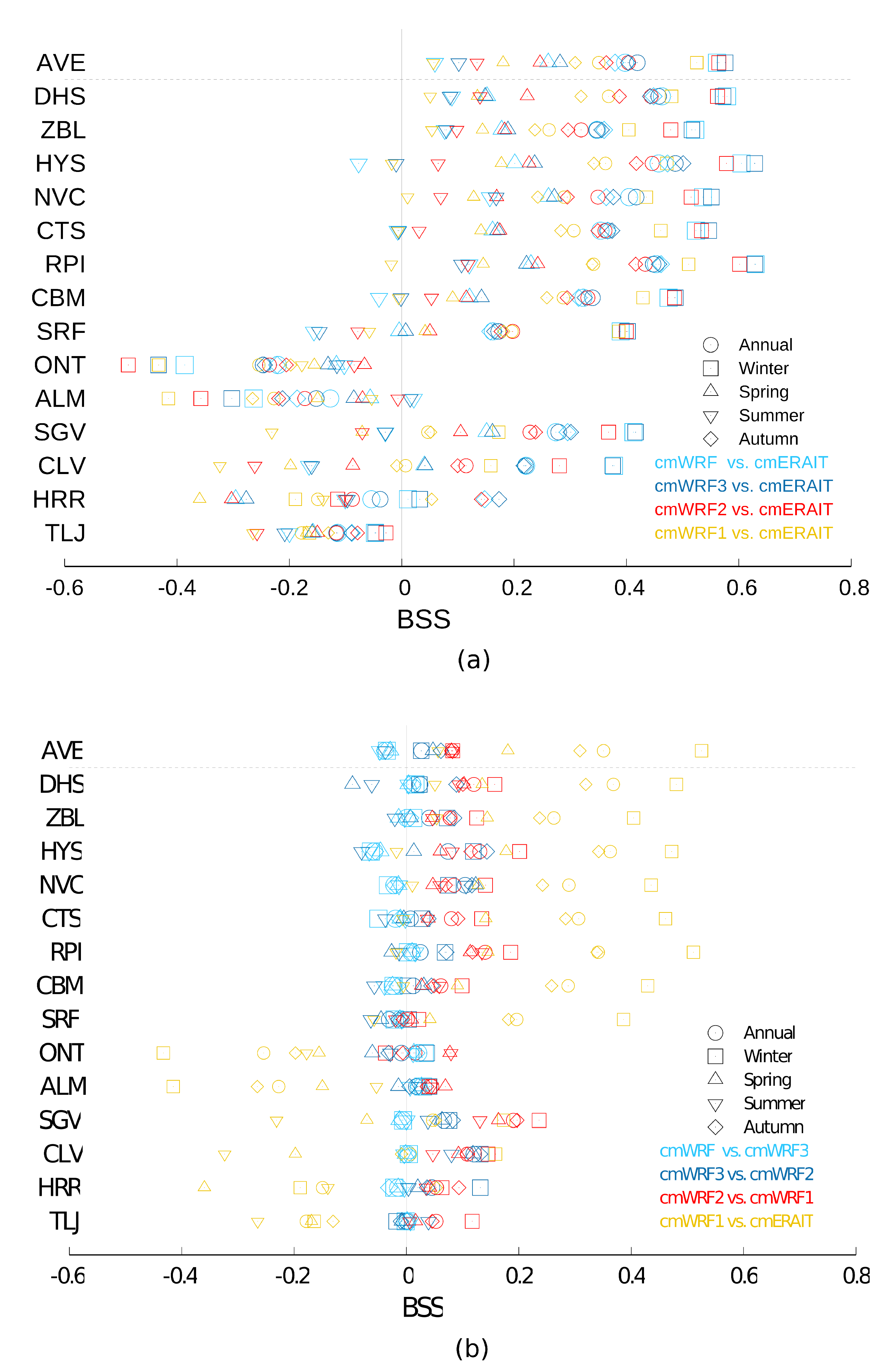
4.1. Model-Observations Comparison
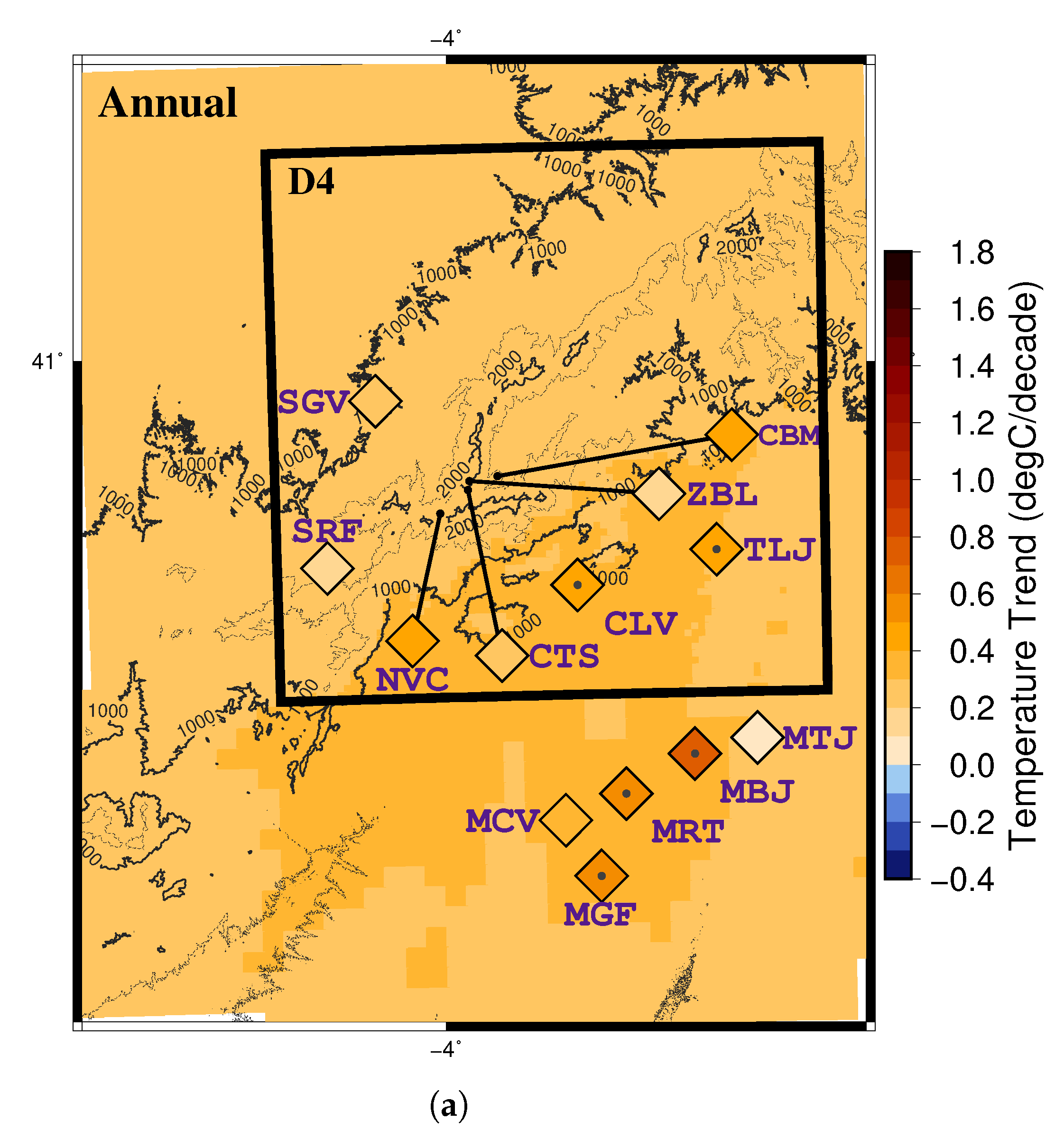
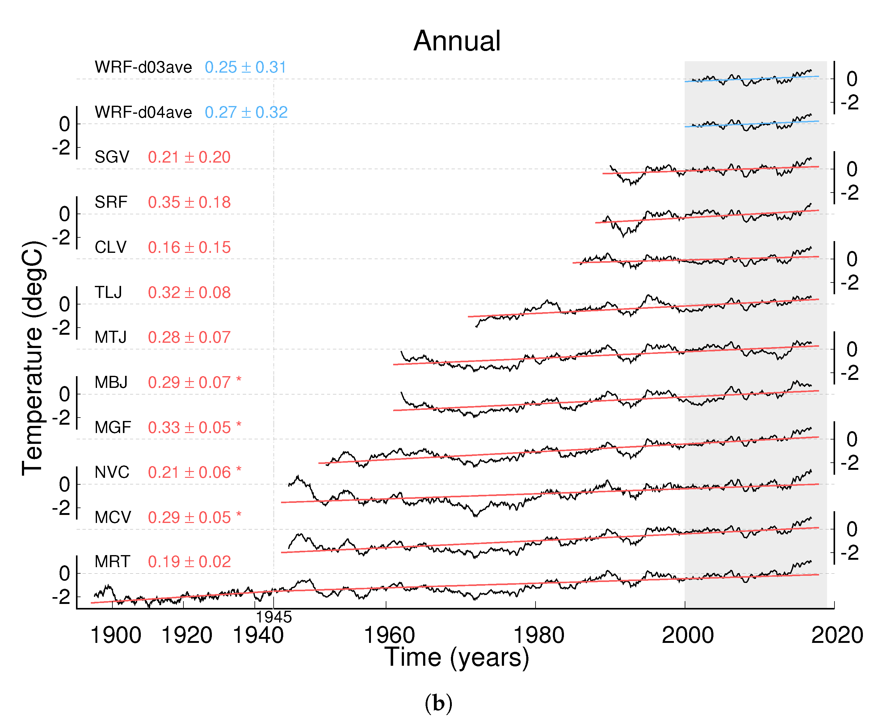
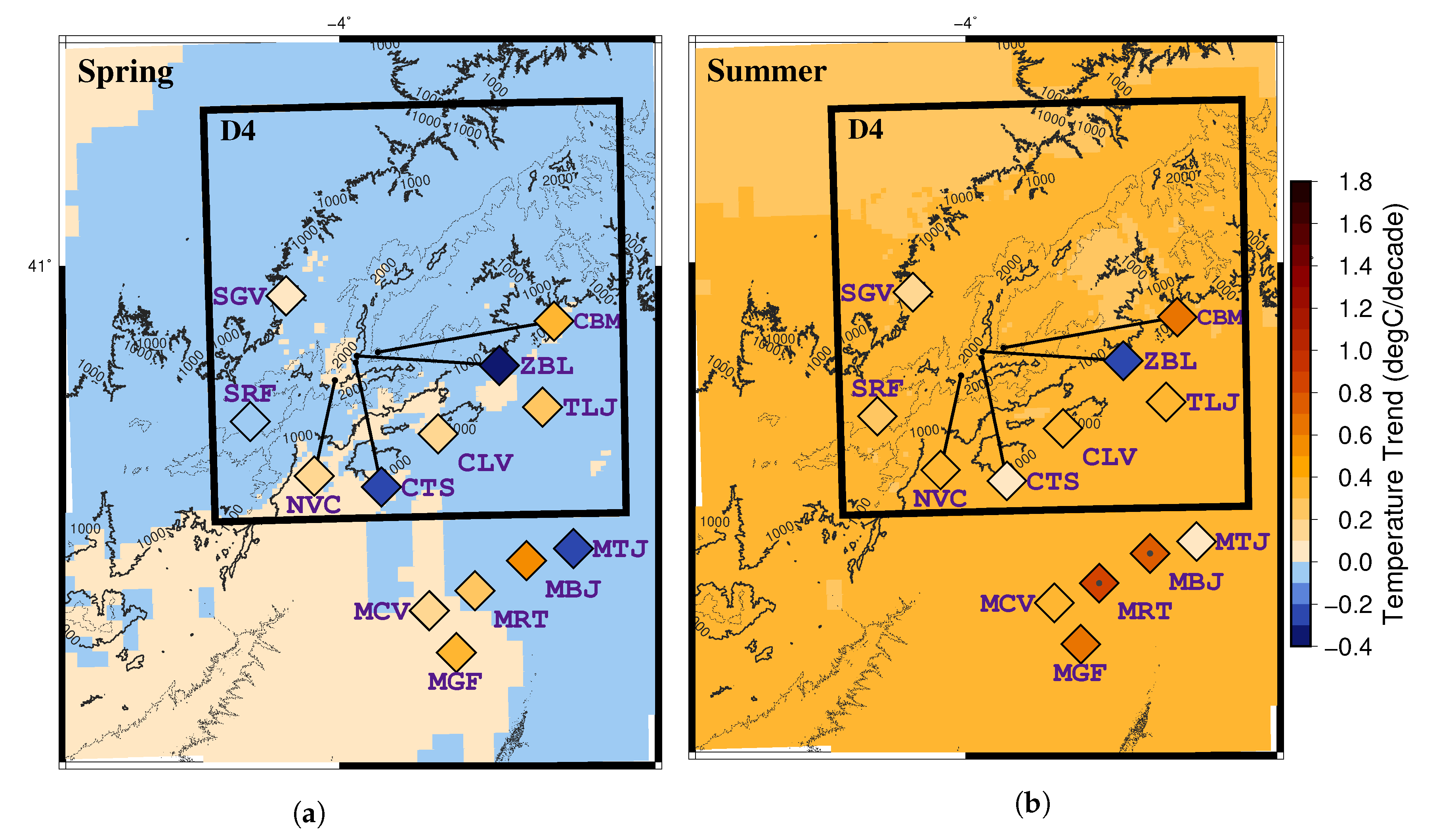
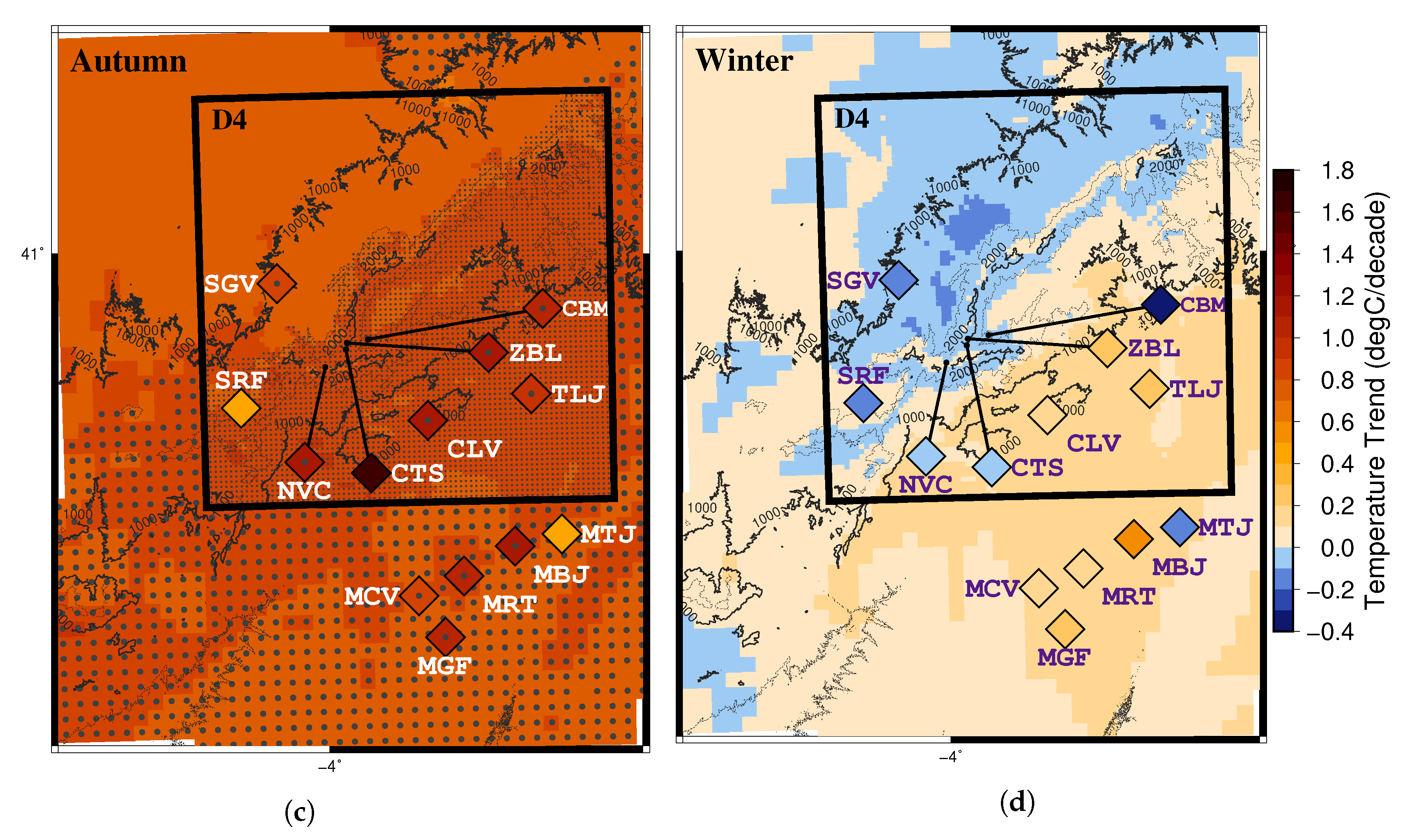
4.2. Temperature-Trend Analysis
5. Conclusions
Author Contributions
Funding
Acknowledgments
Conflicts of Interest
References
- Viviroli, D.; Archer, D.R.; Buytaert, W.; Fowler, H.J.; Greenwood, G.B.; Hamlet, A.F.; Huang, Y.; Koboltschnig, G.; Litaor, M.I.; López-Moreno, J.I.; et al. Climate change and mountain water resources: Overview and recommendations for research, management and policy. Hidrol. Earth Syst. Sci. 2011, 15, 471–504. [Google Scholar] [CrossRef]
- Barry, R.G. Past and potential future changes in mountain environments: A review. In Mountain Environments in Changing Climates; Beniston, M., Ed.; Routledge Taylor & Francis Group: Milton Park, Abingdon, Oxfordshire, UK, 2002; pp. 2–25. [Google Scholar]
- Spehn, E.; Koerner, C. Biodiversity in Mountains: A Natural Heritage Threatened by Climate Change. In Mountains and Climate Change: From Understanding to Action; Kohler, T., Maselli, D., Eds.; Swiss Agency for Development and Cooperation SDC: Bern, Switzerland, 2009; pp. 42–47. [Google Scholar]
- Beniston, M. Mountain Climates and Climatic Change: An Overview of Processes Focusing on the European Alps. Pure Appl. Geophys. 2005, 162, 1587–1606. [Google Scholar] [CrossRef]
- Barry, R.G. Mountain Weather and Climate; Cambridge University Press: Cambridge, UK, 2008. [Google Scholar]
- Shafer, S.L.; Bartlein, P.J.; Whitlock, C. Understanding the Spatial Heterogeneity of Global Environmental Change in Mountain Regions. In Global Change and Mountain Regions. An Overview of Current Knowledge; Huber, U.M., Bugmann, H.K.M., Reasoner, M.A., Eds.; Springer: New York, NY, USA, 2006; pp. 21–30. [Google Scholar]
- Kohler, T.; Wehrli, A.; Jurek, M. Mountains and Climate Change. A Global Concern; Centre for the Development and Environment (CDE), Swiss Agency for Development and Cooperation (SDC) and Geographica Bernensia: Bern, Switzerland, 2014. [Google Scholar]
- Giorgi, F.; Hurrel, J.W.; Marinucci, M.R. Elevation Dependency of the Surface Climate Change Signal: A model study. J. Clim. 1996, 10, 288–296. [Google Scholar] [CrossRef]
- Holland, M.M.; Blitz, C.M. Polar Amplification of Climate Change in Coupled Models. Clim. Dyn. 2003, 21, 221–232. [Google Scholar] [CrossRef]
- Díaz, H.F.; Bradley, R.S. Temperature Variations during the Last Century at High Elevation Sites. In Climatic Change at High Elevation Sites; Díaz, H.F., Beniston, M., Bradley, R.S., Eds.; Springer: Dordrecht, The Netherlands, 1997. [Google Scholar] [CrossRef]
- Ceppi, P.; Scherrer, S.C.; Fischer, A.M.; Appenzeller, C. Revisiting Swiss Temperatures trends 1959–2008. Int. J. Climatol. 2010, 32, 203–213. [Google Scholar] [CrossRef]
- Klemes, V. The Modelling of Mountain Hydrology: The Ultimate Challenge. Int. Assoc. Hydr. Sci. (IAHS) 1990, 190, 29–43. [Google Scholar]
- Lucio-Eceiza, E.E.; González-Rouco, J.F.; García-Bustamante, E.; Navarro, J.; Beltrami, H. Multidecadal to Centennial Surface Wintertime Wind Variability over Northeastern North-America via Statistical Downscaling. Clim. Dyn. 2019, 53, 41–66. [Google Scholar] [CrossRef]
- Zorita, E.; Von Storch, H. The Analog Method as a Simple Statistical Downscaling Technique: Comparison with More Complicated Methods. J. Clim. 1999, 12, 2474–2489. [Google Scholar] [CrossRef]
- González-Rouco, J.F.; Heyen, H.; Zorita, E.; Valero, F. Agreement between Observed Rainfall Trends and Climate Change Simulations in the Southwest of Europe. J. Clim. 2000, 13, 3057–3065. [Google Scholar] [CrossRef][Green Version]
- Rummukainen, M. State-of-the-art with Regional Climate Models. WIREs Clim. Chang. 2010, 1, 82–96. [Google Scholar] [CrossRef]
- Skamarock, W.C.; Klemp, J.B.; Dudhia, J.; Gill, D.; Barker, D.M.; Wang, W.; Powers, J.G. A Description of the Advanced Research WRF Version 2; Technical Report TN-468+STR; NCAR: Boulder, CO, USA, 2005. [Google Scholar]
- Dee, D.P.; Uppala, S.M.; Simmons, A.J.; Berrisford, P.; Poli, P.; Kobayashi, S.; Andrae, U.; Balmaseda, M.; Balsamo, G.; Bauer, P.; et al. The ERA-Interim Reanalysis: Configuration and Performance of the Data Assimilation System. Q. J. R. Meteorol. Soc. 2011, 137, 553–597. [Google Scholar] [CrossRef]
- IPCC. Global Warming of 1.5 °C. An IPCC Special Report in the Impacts of Global Warming of 1.5 °C Above Pre-Industrial Levels and Related Global Greenhouse Gas Emission Pathways, in the Context of Strengthening the Global Response to the Threat of Climate Change, Sustainable Development, and Efforts to Eradicate Poverty; Masson-Delmotte, V., Zhai, P., Portner, H.O., Roberts, D., Skea, J., Shukla, P.R., Pirani, A., Moufouma-Okia, W., Pèan, C., Pidcock, R., Eds.; IPCC: Geneva, Switzerland, 2018; in press. [Google Scholar]
- González-Hidalgo, J.C.; Peña-Angulo, D.; Brunetti, M.; Cortesi, N. Recent Trend in Temperature Evolution in Spanish mainland (1951–2010): From Warming to Hiatus. Int. J. Climatol. 2016, 36, 2405–2416. [Google Scholar] [CrossRef]
- Brunet, M.; Jones, P.D.; Sigró, J.; Saladié, O.; Aguilar, E.; Moberg, A.; Della-Marta, P.M.; Lister, D.; Walther, A.; López, D. Temporal and Spatial Temperature Variability and Change over Spain during 1850–2005. J. Geophys. Res. 2007, 112. [Google Scholar] [CrossRef]
- Cuchiara, G.C.; Rappengluck, B. Performace Analysis of WRF and LES in Describing the Evolution and Structure of the Planetary Boundary Layer. Environ. Fluid Mech. 2018, 18, 1257–1273. [Google Scholar] [CrossRef]
- Berrisford, P.; Dee, D.; Poli, P.; Brugge, R.; Fielding, K.; Fuentes, M.; Kallberg, P.; Kobayasi, S.; Uppala, S.; Simmons, A. The ERA-Interim archive Version 2.0; ECMWF ERA Rep. Ser. 1: Reading, UK, 2011. [Google Scholar]
- Iacono, M.J.; Delamere, J.S.; Mlawer, E.J.; Shephard, M.W.; Clough, S.A.; Collins, W.D. Radiative Forcing by Long-lived Greenhouse Gases: Calculations with the AER Radiative Transfer Models. J. Geophys. Res. 2008, 113. [Google Scholar] [CrossRef]
- Kain, J.S.; Fritsch, J.M. A One-Dimensional Entraining/Detraining Plume Model and Its Application in Convective Parameterization. J. Atmospher. Sci. 1990, 47, 2784–2802. [Google Scholar] [CrossRef]
- Kain, J.S.; Fritsch, J.M. Convective Parameterization for Mesoscale Models: The Kain-Fritsch Scheme. In The Representation of Cumulus Convection in Numerical Models; Emanuel, K.A., Raymond, D.J., Eds.; Am. Meteorol. Soc.: Boston, MA, USA, 1993; pp. 165–170. [Google Scholar]
- Hong, S.Y.; Noh, Y.; Dudhia, J. A New Vertical Diffusion Package with an Explicit Treatment of Entrainment Processes. Mon. Weather Rev. 2006, 134, 2318–2341. [Google Scholar] [CrossRef]
- Lin, Y.L.; Farley, R.D.; Orville, H.D. Bulk Parameterization of the Snow Field in Cloud Model. J. Appl. Meteor. Climatol. 1983, 22, 1065–1092. [Google Scholar] [CrossRef]
- Chen, F.; Dudhia, J. Coupling an Advanced Land-Surface/Hydrology Model with the Penn State/NCAR MM5 Modelling System. Part I: Model Implementation and Sensitivity. Mon. Weather Rev. 2001, 129, 569–585. [Google Scholar] [CrossRef]
- Monin, A.S.; Obukhov, A. Basic Laws of Turbulent Mixing in the Surface Layer of the Atmosphere. Contrib. Geophys. Inst. Acad. Sci. USSR 1954, 151, 163–187. (In Russian) [Google Scholar]
- Carlson, T.N.; Boland, F.E. Analysis of Urban-Rural Canopy using a Surface Heat Flux/Temperature Model. J. Appl. Meteor. 1978, 17, 998–1013. [Google Scholar] [CrossRef]
- Jiménez, P.A.; Dudhia, J.; González-Rouco, J.F.; Navarro, J.; Montávez, J.P.; García-Bustamante, E. A Revised Scheme for the WRF Surface Layer Formulation. Mon. Weather Rev. 2012, 140, 898–918. [Google Scholar] [CrossRef]
- Anderson, J.R.; Hardy, E.E.; Roach, J.T.; Witmer, R.E. A Land Use and Land Cover Classification System for Use with Remote Sensor Data; Geol. Surv. Prof. Paper 964 (US Government Printing Office): Washington, DC, USA, 1976.
- Bliss, N.B.; Olsen, L.M. Development of a 30-arc-second Digital Elevation Model of South America. In Proceedings of the Pecora Thirteen, Human Interactions with the Environment-Perspectives from Space, Sioux Falls, SD, USA, 20–22 August 1996. [Google Scholar]
- Gesch, D.B.; Larson, K.S. Techniques for Development of Global 1-Kilometer Digital Elevation Models. In Proceedings of the Pecora Thirteen, Human Interactions with the Environment-Perspectives from Space, Sioux Falls, SD, USA, 20–22 August 1996. [Google Scholar]
- Verdin, K.L.; Greenlee, S.K. Development of Continental Scale Digital Elevation Models and Extraction of Hydrographic Features. In Proceedings of the Third International Conference/Workshop on Integrating GIS and Environmental Modeling, Santa Fe, NM, USA, 21–26 January 1996. [Google Scholar]
- Jiménez, P.A.; González-Rouco, J.F.; Bustamante, E.G.; Navarro, J.; Montávez, J.P.; de Arellano, J.V.G.; Dudhia, J.; Roldán, A. Surface Wind Regionalization Over Complex Terrain: Evaluation and Analysis of a High Resolution WRF Simulation. J. Appl. Meteorol. 2010, 49, 268–287. [Google Scholar] [CrossRef]
- Universidad Complutense de Madrid (UCM). GuMNet—Guadarrama Monitoring Network. Available online: https://www.ucm.es/gumnet (accessed on 10 September 2020).
- Lucio-Eceiza, E.E.; González-Rouco, J.F.; Navarro, J.; Beltrami, H. Quality Control of Surface Wind Observations in Northeastern North America. Part I: Data Management Issues. J. Atmos. Oceanic Technol. 2018, 35, 163–182. [Google Scholar] [CrossRef]
- Lucio-Eceiza, E.E.; González-Rouco, J.F.; Navarro, J.; Beltrami, H.; Conte, J. Quality Control of Surface Wind Observations in Northeastern North America. Part II: Measurement Errors. J. Atmos. Oceanic Technol. 2018, 35, 183–205. [Google Scholar] [CrossRef]
- Taylor, K.E. Summarizing multiple aspects of model performance in a single diagram. J. Geophys. Res. Atmos. 2001, 106, 7183–7192. [Google Scholar] [CrossRef]
- Von Storch, H.; Zwiers, F.W. Statistical Analysis in Climate Research; Cambridge University Press: Cambridge, UK, 1999. [Google Scholar]
- Osborn, T.J.; Briffa, K.R.; Jones, P.D. Adjusting Variance for Sample-size in Tree-ring Chronologies and Other Regional Mean Timeseries. Dendrochronology 1997, 15, 89–99. [Google Scholar]
- Jiménez, P.A.; González-Rouco, J.F.; Montávez, J.P.; Navarro, J.; García-Bustamante, E.; Dudhia, J. Analysis of the long-term Surface Wind Variability over Complex Terrain using a High Spatial Resolution WRF Simulation. Clim. Dyn. 2013, 40, 1634–1656. [Google Scholar] [CrossRef]
- Xoplaki, E.; González-Rouco, J.F.; Luterbacher, J.; Wanner, H. Mediterranean Summer Air Temperature Variability and its Connection to the Large-Scale Atmospheric Circulation and SSTs. Clim. Dyn. 2003, 20, 723–739. [Google Scholar] [CrossRef]
- Kambezidis, H.D.; Kaskaoutis, D.G.; Kalliampakos, G.K.; Rashki, A.; Wild, M. The Solar Dimming/Brightening Effect over the Mediterranean Basin in the period 1979–2012. J. Atmos. Solar-Terrestr. Phys. 2016, 150, 31–46. [Google Scholar] [CrossRef]


| Observations | ||||||||
|---|---|---|---|---|---|---|---|---|
| Name | Code | Source | Longitude (°) | Latitude (°) | Altitude (masl) | Start Date | Finish Date | WRF Domain |
| Madrid Torrejón | MTJ | AEMet | −3.444 | 40.489 | 607 | 1 January 1961 | 1 November 2018 | D3 |
| Madrid Barajas | MBJ | AEMet | −3.556 | 40.467 | 609 | 1 January 1961 | 1 November 2018 | D3 |
| Madrid Getafe | MGF | AEMet | −3.722 | 40.299 | 620 | 1 January 1951 | 31 October 2018 | D3 |
| Talamanca del Jarama | TLJ | AEMet | −3.517 | 40.745 | 654 | 1 January 1970 | 30 September 2018 | D4 |
| Madrid Retiro | MRT | AEMet | −3.678 | 40.412 | 667 | 1 March 1893 | 31 October 2018 | D3 |
| Madrid Cuatro Vientos | MCV | AEMet | −3.786 | 40.376 | 690 | 1 May 1945 | 1 November 2018 | D3 |
| Herrería | HRR | GuMNet | −4.136 | 40.582 | 920 | 7 June 2016 | 31 August 2018 | D4 |
| Colmenar Viejo | CLV | AEMet | −3.765 | 40.696 | 1004 | 1 January 1985 | 1 November 2018 | D4 |
| Segovia | SGV | AEMet | −4.126 | 40.945 | 1005 | 1 January 1988 | 1 November 2018 | D4 |
| Alameda | ALM | GuMNet | −3.844 | 40.915 | 1115 | 2 October 2009 | 31 August 2018 | D4 |
| Ontalva | ONT | PNP | −3.893 | 40.872 | 1188 | 22 February 2008 | 19 September 2014 | D4 |
| San Rafael | SRF | AEMet | −4.212 | 40.719 | 1237 | 1 January 1987 | 31 October 2018 | D4 |
| Cabeza Mediana | CBM | GuMNet | −3.908 | 40.844 | 1682 | 2 October 2009 | 31 August 2018 | D4 |
| Raso del Pino I | RPI | GuMNet | −3.969 | 40.874 | 1803 | 26 July 2014 | 31 August 2018 | D4 |
| Cotos | CTS | GuMNet | −3.961 | 40.825 | 1873 | 1 January 2005 | 31 August 2018 | D4 |
| Navacerrada | NVC | AEMet | −4.011 | 40.793 | 1894 | 1 January 1946 | 1 November 2018 | D4 |
| Hoyas | HYS | GuMNet | −3.955 | 40.834 | 2019 | 30 October 2014 | 31 August 2018 | D4 |
| Zabala | ZBL | GuMNet | −3.958 | 40.837 | 2075 | 1 January 2000 | 31 August 2018 | D4 |
| Dos Hermanas | DHS | GuMNet | −3.964 | 40.837 | 2225 | 9 October 2014 | 23 January 2018 | D4 |
| cWRF | cERAIT | |||||||
|---|---|---|---|---|---|---|---|---|
| Name | Code | Long (°) | Lat (°) | Altitude (masl) | Code | Long (°) | Lat (°) | Altitude (masl) |
| Madrid Torrejón | MTJ | −3.439 | 40.478 | 585 | ERAIT1 | −3.750 | 40.500 | 855 |
| Madrid Barajas | MBJ | −3.548 | 40.476 | 584 | ERAIT1 | −3.750 | 40.500 | 855 |
| Madrid Getafe | MGF | −3.727 | 40.306 | 603 | ERAIT1 | −3.750 | 40.500 | 855 |
| Talamanca del Jarama | TLJ | −3.518 | 40.746 | 643 | ERAIT1 | −3.750 | 40.500 | 855 |
| Madrid Retiro | MRT | −3.693 | 40.418 | 639 | ERAIT1 | −3.750 | 40.500 | 855 |
| Madrid Cuatro Vientos | MCV | −3.802 | 40.389 | 674 | ERAIT1 | −3.750 | 40.500 | 855 |
| Herrería | HRR | −4.138 | 40.586 | 993 | ERAIT3 | −4.500 | 40.500 | 856 |
| Colmenar Viejo | CLV | −3.762 | 40.695 | 944 | ERAIT1 | −3.750 | 40.500 | 855 |
| Segovia | SGV | −4.126 | 40.949 | 974 | ERAIT4 | −4.500 | 41.250 | 902 |
| Alameda | ALM | −3.842 | 40.917 | 1084 | ERAIT2 | −3.750 | 41.250 | 997 |
| Ontalva | ONT | −3.890 | 40.870 | 1186 | ERAIT1 | −3.750 | 40.500 | 855 |
| San Rafael | SRF | −4.216 | 40.715 | 1285 | ERAIT3 | −4.500 | 40.500 | 856 |
| Cabeza Mediana | CBM | −3.914 | 40.841 | 1487 | ERAIT1 | −3.750 | 40.500 | 855 |
| Raso del Pino I | RPI | −3.964 | 40.878 | 1918 | ERAIT1 | −3.750 | 40.500 | 855 |
| Cotos | CTS | −3.962 | 40.822 | 1788 | ERAIT1 | −3.750 | 40.500 | 855 |
| Navacerrada | NVC | −4.010 | 40.793 | 1781 | ERAIT1 | −3.750 | 40.500 | 855 |
| Hoyas | HYS | −3.950 | 40.831 | 1710 | ERAIT1 | −3.750 | 40.500 | 855 |
| Zabala | ZBL | −3.963 | 40.840 | 2092 | ERAIT1 | −3.750 | 40.500 | 855 |
| Dos Hermanas | DHS | −3.963 | 40.840 | 2092 | ERAIT1 | −3.750 | 40.500 | 855 |
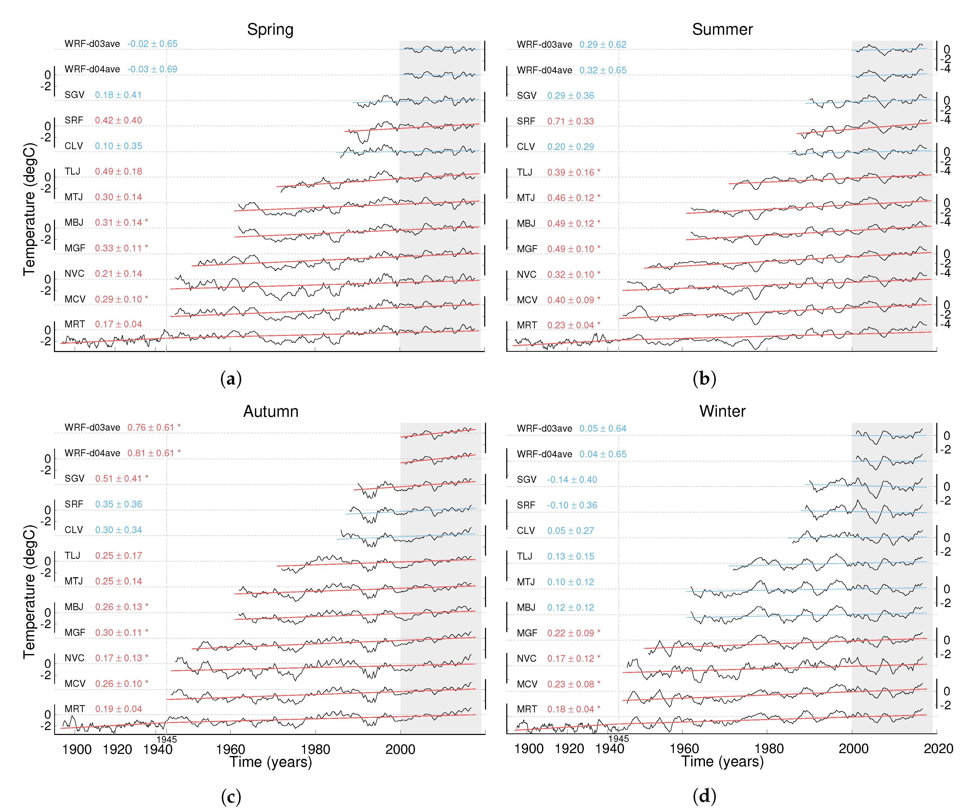
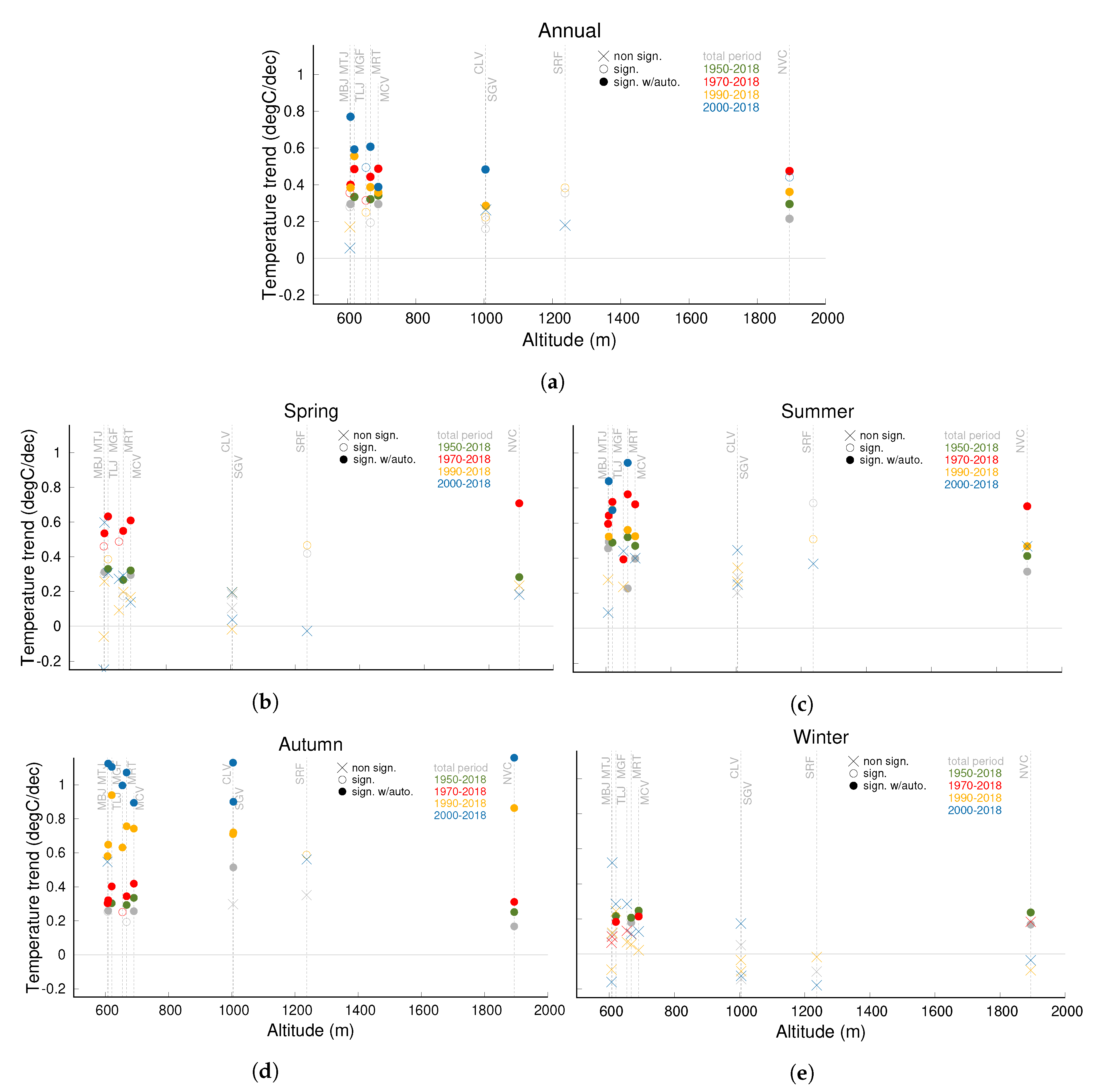
| MONTHLY ANOMALIES TRENDS (°C/decade) | ||||||
|---|---|---|---|---|---|---|
| Name | Total Period | 1950–2018 | 1970–2018 | 1990–2018 | 2000–2018 | |
| WRF D3 average | Annual | 0.25 ± 0.31 | - | - | - | - |
| Spring | −0.02 ± 0.65 | - | - | - | - | |
| Summer | 0.29 ± 0.62 | - | - | - | - | |
| Autumn | ** 0.76 ± 0.61 | - | - | - | - | |
| Winter | 0.05 ± 0.64 | - | - | - | - | |
| WRF D4 average | Annual | 0.27 ± 0.32 | - | - | - | - |
| Spring | −0.02 ± 0.69 | - | - | - | - | |
| Summer | 0.32 ± 0.65 | - | - | - | - | |
| Autumn | ** 0.81 ± 0.61 | - | - | - | - | |
| Winter | 0.03 ± 0.65 | - | - | - | - | |
| Segovia | Annual | * 0.21 ± 0.20 | - | - | ** 0.28 ± 0.21 | 0.26 ± 0.37 |
| Spring | 0.18 ± 0.41 | - | - | 0.20 ± 0.42 | 0.04 ± 0.79 | |
| Summer | 0.29 ± 0.36 | - | - | 0.34 ± 0.38 | 0.25 ± 0.70 | |
| Autumn | ** 0.51 ± 0.41 | - | - | ** 0.72 ± 0.43 | ** 0.90 ± 0.68 | |
| Winter | −0.14 ± 0.40 | - | - | −0.10 ± 0.41 | −0.12 ± 0.82 | |
| San Rafael | Annual | * 0.35 ± 0.18 | - | - | * 0.38 ± 0.21 | 0.18 ± 0.35 |
| Spring | * 0.42 ± 0.40 | - | - | * 0.47 ± 0.46 | −0.03 ± 0.71 | |
| Summer | * 0.71 ± 0.33 | - | - | * 0.51 ± 0.36 | 0.37 ± 0.65 | |
| Autumn | 0.35 ± 0.36 | - | - | * 0.59 ± 0.40 | 0.56 ± 0.65 | |
| Winter | −0.10 ± 0.36 | - | - | −0.02 ± 0.41 | −0.18 ± 0.81 | |
| Colmenar Viejo | Annual | * 0.16 ± 0.15 | - | - | * 0.22 ± 0.19 | ** 0.48 ± 0.33 |
| Spring | 0.10 ± 0.35 | - | - | −0.02 ± 0.42 | 0.19 ± 0.77 | |
| Summer | 0.20 ± 0.29 | - | - | 0.27 ± 0.35 | 0.44 ± 0.64 | |
| Autumn | 0.30 ± 0.33 | - | - | ** 0.71 ± 0.37 | ** 1.13 ± 0.58 | |
| Winter | 0.05 ± 0.27 | - | - | −0.03 ± 0.33 | 0.17 ± 0.65 | |
| Talamanca del Jarama | Annual | * 0.31 ± 0.08 | - | * 0.31 ± 0.08 | * 0.25 ± 0.17 | * 0.49 ± 0.30 |
| Spring | * 0.49 ± 0.18 | - | * 0.49 ± 0.18 | 0.09 ± 0.36 | 0.27 ± 0.71 | |
| Summer | ** 0.39 ± 0.16 | - | ** 0.39 ± 0.16 | 0.24 ± 0.32 | 0.44 ± 0.60 | |
| Autumn | * 0.25 ± 0.17 | - | * 0.25 ± 0.17 | ** 0.63 ± 0.33 | ** 1.00 ± 0.54 | |
| Winter | 0.13 ± 0.15 | - | 0.13 ± 0.15 | 0.07 ± 0.31 | 0.28 ± 0.57 | |
| Madrid Torrejón | Annual | * 0.28 ± 0.07 | - | * 0.36 ± 0.08 | 0.17 ± 0.17 | 0.05 ± 0.31 |
| Spring | * 0.30 ± 0.14 | - | * 0.46 ± 0.17 | −0.06 ± 0.36 | −0.25 ± 0.69 | |
| Summer | ** 0.46 ± 0.12 | - | ** 0.60 ± 0.16 | 0.28 ± 0.34 | 0.09 ± 0.64 | |
| Autumn | * 0.25 ± 0.13 | - | ** 0.30 ± 0.17 | ** 0.58 ± 0.34 | 0.55 ± 0.56 | |
| Winter | 0.10 ± 0.12 | - | 0.06 ± 0.15 | −0.09 ± 0.32 | −0.16 ± 0.60 | |
| Madrid Barajas | Annual | ** 0.29 ± 0.06 | - | ** 0.40 ± 0.08 | ** 0.38 ± 0.17 | ** 0.77 ± 0.30 |
| Spring | ** 0.31 ± 0.13 | - | ** 0.53 ± 0.17 | 0.26 ± 0.35 | 0.60 ± 0.69 | |
| Summer | ** 0.49 ± 0.12 | - | ** 0.64 ± 0.15 | ** 0.52 ± 0.32 | ** 0.84 ± 0.60 | |
| Autumn | ** 0.26 ± 0.13 | - | ** 0.32 ± 0.16 | ** 0.65 ± 0.34 | ** 1.12 ± 0.56 | |
| Winter | 0.11 ± 0.12 | - | 0.10 ± 0.15 | 0.12 ± 0.32 | 0.52 ± 0.58 | |
| Madrid Getafe | Annual | ** 0.33 ± 0.05 | ** 0.33 ± 0.05 | ** 0.48 ± 0.08 | ** 0.56 ± 0.17 | ** 0.59 ± 0.30 |
| Spring | ** 0.33 ± 0.11 | ** 0.33 ± 0.11 | ** 0.63 ± 0.18 | * 0.39 ± 0.38 | 0.31 ± 0.71 | |
| Summer | ** 0.49 ± 0.09 | ** 0.49 ± 0.09 | ** 0.72 ± 0.15 | ** 0.68 ± 0.34 | ** 0.67 ± 0.62 | |
| Autumn | ** 0.30 ± 0.11 | ** 0.30 ± 0.11 | ** 0.40 ± 0.17 | ** 0.94 ± 0.34 | ** 1.10 ± 0.54 | |
| Winter | ** 0.22 ± 0.09 | ** 0.22 ± 0.09 | ** 0.18 ± 0.14 | 0.24 ± 0.30 | 0.28 ± 0.58 | |
| Navacerrada | Annual | ** 0.21 ± 0.06 | ** 0.29 ± 0.07 | ** 0.47 ± 0.11 | ** 0.36 ± 0.23 | * 0.44 ± 0.40 |
| Spring | * 0.21 ± 0.14 | ** 0.28 ± 0.15 | ** 0.71 ± 0.24 | 0.23 ± 0.51 | 0.18 ± 0.92 | |
| Summer | ** 0.32 ± 0.10 | ** 0.41 ± 0.11 | ** 0.70 ± 0.19 | ** 0.47 ± 0.39 | 0.47 ± 0.70 | |
| Autumn | ** 0.17 ± 0.13 | ** 0.25 ± 0.14 | ** 0.31 ± 0.23 | ** 0.86 ± 0.47 | ** 1.16 ± 0.75 | |
| Winter | ** 0.17 ± 0.12 | ** 0.24 ± 0.12 | 0.18 ± 0.20 | −0.09 ± 0.45 | −0.04 ± 0.87 | |
| Madrid Cuatro Vientos | Annual | ** 0.29 ± 0.05 | ** 0.34 ± 0.05 | ** 0.49 ± 0.09 | ** 0.36 ± 0.18 | ** 0.39 ± 0.31 |
| Spring | ** 0.29 ± 0.10 | ** 0.32 ± 0.11 | ** 0.61 ± 0.19 | 0.17 ± 0.39 | 0.14 ± 0.73 | |
| Summer | ** 0.40 ± 0.09 | ** 0.47 ± 0.10 | ** 0.71 ± 0.16 | ** 0.52 ± 0.35 | 0.40 ± 0.65 | |
| Autumn | ** 0.26 ± 0.10 | ** 0.33 ± 0.11 | ** 0.42 ± 0.18 | ** 0.74 ± 0.35 | ** 0.89 ± 0.55 | |
| Winter | ** 0.23 ± 0.08 | ** 0.25 ± 0.09 | ** 0.21 ± 0.14 | 0.02 ± 0.31 | 0.13 ± 0.60 | |
| Madrid Retiro | Annual | * 0.19 ± 0.02 | ** 0.32 ± 0.05 | ** 0.44 ± 0.09 | ** 0.39 ± 0.18 | ** 0.61 ± 0.31 |
| Spring | * 0.17 ± 0.04 | ** 0.27 ± 0.11 | ** 0.55 ± 0.18 | 0.20 ± 0.38 | 0.29 ± 0.73 | |
| Summer | ** 0.23 ± 0.04 | ** 0.52 ± 0.09 | ** 0.76 ± 0.16 | ** 0.56 ± 0.36 | ** 0.94 ± 0.65 | |
| Autumn | * 0.19 ± 0.04 | ** 0.29 ± 0.10 | ** 0.34 ± 0.17 | ** 0.76 ± 0.34 | ** 1.07 ± 0.53 | |
| Winter | ** 0.18 ± 0.04 | ** 0.21 ± 0.09 | 0.11 ± 0.13 | 0.05 ± 0.30 | 0.11 ± 0.59 | |
© 2020 by the authors. Licensee MDPI, Basel, Switzerland. This article is an open access article distributed under the terms and conditions of the Creative Commons Attribution (CC BY) license (http://creativecommons.org/licenses/by/4.0/).
Share and Cite
Vegas-Cañas, C.; González-Rouco, J.F.; Navarro-Montesinos, J.; García-Bustamante, E.; Lucio-Eceiza, E.E.; García-Pereira, F.; Rodríguez-Camino, E.; Chazarra-Bernabé, A.; Álvarez-Arévalo, I. An Assessment of Observed and Simulated Temperature Variability in Sierra de Guadarrama. Atmosphere 2020, 11, 985. https://doi.org/10.3390/atmos11090985
Vegas-Cañas C, González-Rouco JF, Navarro-Montesinos J, García-Bustamante E, Lucio-Eceiza EE, García-Pereira F, Rodríguez-Camino E, Chazarra-Bernabé A, Álvarez-Arévalo I. An Assessment of Observed and Simulated Temperature Variability in Sierra de Guadarrama. Atmosphere. 2020; 11(9):985. https://doi.org/10.3390/atmos11090985
Chicago/Turabian StyleVegas-Cañas, Cristina, J. Fidel González-Rouco, Jorge Navarro-Montesinos, Elena García-Bustamante, Etor E. Lucio-Eceiza, Félix García-Pereira, Ernesto Rodríguez-Camino, Andrés Chazarra-Bernabé, and Inés Álvarez-Arévalo. 2020. "An Assessment of Observed and Simulated Temperature Variability in Sierra de Guadarrama" Atmosphere 11, no. 9: 985. https://doi.org/10.3390/atmos11090985
APA StyleVegas-Cañas, C., González-Rouco, J. F., Navarro-Montesinos, J., García-Bustamante, E., Lucio-Eceiza, E. E., García-Pereira, F., Rodríguez-Camino, E., Chazarra-Bernabé, A., & Álvarez-Arévalo, I. (2020). An Assessment of Observed and Simulated Temperature Variability in Sierra de Guadarrama. Atmosphere, 11(9), 985. https://doi.org/10.3390/atmos11090985