Article

A Nonlinear Land Use Regression Approach for Modelling NO2 Concentrations in Urban Areas—Using Data from Low-Cost Sensors and Diffusion Tubes

1
Department of Civil and Structural Engineering, the University of Sheffield, Sheffield S1 3JD, UK
2
Department of Automatic Control and Systems Engineering, the University of Sheffield, Sheffield S1 3JD, UK
*
Author to whom correspondence should be addressed.
Atmosphere 2020, 11(7), 736; https://doi.org/10.3390/atmos11070736
Submission received: 8 June 2020 / Revised: 8 July 2020 / Accepted: 9 July 2020 / Published: 11 July 2020
(This article belongs to the Special Issue Air Quality in the UK)

Abstract

:
Land Use Regression (LUR) based on multiple linear regression model is one of the techniques used most frequently for modelling the spatial variability of air pollution and assessing exposure in urban areas. In this paper, a nonlinear generalised additive model is proposed for LUR and its performance is compared to a linear model in Sheffield, UK for the year 2019. Pollution models were estimated using NO2 measurements obtained from 188 diffusion tubes and 40 low-cost sensors. Performance of the models was assessed by calculating several statistical metrics including correlation coefficient (R) and root mean square error (RMSE). High resolution (100 m × 100 m) maps demonstrated higher levels of NO2 in the city centre, eastern side of the city and on major roads. The results showed that the nonlinear model outperformed the linear counterpart and that the model estimated using NO2 data from diffusion tubes outperformed the models using data from low-cost sensors or both low-cost sensors and diffusion tubes. The proposed method provides a basis for further application of advanced nonlinear modelling approaches to constructing LUR models in urban areas which enable quantifying small scale variability in pollution levels.

1. Introduction

Air pollution is one of the serious environmental issues that affects human health and may cause mortality. Landrigan [1] reported that air pollution caused 64 million deaths worldwide in 2015, which shows the significance of the impact of poor air quality on human health. Several air pollutants are shown to have negative impacts on human health, however, among gaseous pollutants nitrogen dioxide (NO2) is considered the most serious pollutant causing both chronic and acute respiratory diseases including asthma, hospital admission and mortality [2]. NO2 is considered the most serious gaseous pollutant in urban areas and many air quality management areas (AQMAs) in the UK are based on the exceedances of NO2 [3]. Therefore, it is important to carry out different monitoring and modelling investigations to analyse its spatial variability, especially micro-level variability. This could be done by developing high resolution maps in urban areas that help in understanding the main drivers of NO2 levels and quantifying exposure to elevated NO2 concentrations in urban areas. It is not feasible to capture micro-level spatial variability in NO2 concentration with the help of monitoring network in a large urban area as this requires a huge number of sensors. Alternatively, a certain number of sensors can be installed, and the concentrations can be extrapolated to other areas using modelling techniques. This is exactly what this study intends to do.
One of the challenges of air pollution in urban areas is the quantification of small-scale local level exposure by analysing spatial variability in pollutant concentrations. The small scale variability in urban areas is controlled by emission sources, land use features, building density-and-height and geographical characteristics. To characterise spatial variability in pollutant concentrations, three approaches are most commonly used: GIS (Geographical Information Systems) based interpolation methods, Dispersion models, and land use regression (LUR) models.
Hsu et al. [4] reviewed different methods used for interpolation and divided them into two categories: Geostatistical and Non-geostatistical methods. The geostatistical techniques include Ordinary Kriging, Universal Kriging, Simple Kriging, Empirical Bayesian Kriging and Original CoKriging. The non-geostatistical techniques include Splines, Trend Surface Analysis, Inverse Distance Weighting and Natural Neighbour. According to the findings of Hsu et al. [4] the geostatistical interpolations showed better prediction than the non-geostatistical interpolation techniques. Interpolation methods are used to interpolate air pollutant concentrations between various air monitoring stations to provide better spatial coverage. However, when these approaches are applied at a local scale such as intra-city scale, these methodologies are known to produce considerable variations in air pollutant concentrations within a small area and are more effective at large scales, such as national or regional scale [5]. Therefore, at urban scale interpolation approaches should not be the priority for analysing spatial variability of air pollution.
Dispersion models are probably the most advanced modelling techniques for determining the spatial variability of air pollutants in urban areas. Dispersion models combine the data of pollutant emission from different sources (e.g., point, line and area sources), the geophysical characteristics of the study area and meteorological parameters. Dispersion models have the potential to incorporate both temporal and spatial variations to replace the need for air pollution monitoring. However, high cost of purchase and maintenance, high input demands, and requirement of skilled staff limit their application.
LUR models provide an effective alternative to GIS interpolation and dispersion modelling techniques on urban scale. LUR is a spatial modelling approach used most frequently for analysing the spatial variability and quantifying public exposure to air pollution in urban areas. Different modelling, mapping and data fusion techniques are available for modelling spatial variability of air pollution in urban areas [6]. Several authors have preferred Land Use Regression (LUR) over other approaches. Briggs et al. [7] compared the performance of LUR with spatial interpolation methods (e.g., kriging, TIN-contouring and trend surface analysis) and reported that LUR performed much better than the interpolation techniques. The reason was that in urban areas spatial variability of air pollutants is more controlled by the local emission sources and geographical characteristics, rather than a smoothly varying field which is assumed by the interpolation methods. Hoek et al. [8] reviewed several LUR models and reported that the performance of the LUR model in urban areas was either equivalent or better than dispersion and geostatistical approaches. LUR is a widely employed approach for air pollution exposure estimation using Geographical Information Systems (GIS) and statistical analyses to determine the association between geographic features and measured atmospheric pollutant concentrations [9]. LUR is easy to implement and can provide an effective alternative to geostatistical and dispersion modelling techniques on urban scale. LUR approach was introduced by Briggs et al. [9] and since then has been used in numerous studies around the world [8,10,11,12,13,14,15,16]. LUR models associate pollutant concentrations, such as NO2 to site specific geographical characteristics, e.g., topography, land use, traffic, population density, altitude and meteorological parameters. The use of these variables in the regression model are known to capture small scale variability on city scale [17]. Recent development in GIS technology has also added to the popularity of LUR approaches.
Rahman et al. [13] developed an LUR model in Brisbane, Australia to predict NO2 and NOx during 2009–2012. The model was able to explain 64% and 70% variations in NO2 and NOx, respectively. Distance to major roads and industrial areas were the common predictor variables for both NO2 and NOx, suggesting an important role of road traffic and industrial emissions. Rahman et al. [13] used the following independent variables in their model: distance to coast (km), distance to port (km), distance to airport (km), distance to nearest major road (km), distance to nearest minor road (km), major road length (km), minor road length (km), population density (person/km2), land use by type (km2), and elevation (m). Muttoo et al. [12] used several geographic predictor variables to predict NOx levels in Durban, South Africa employing an LUR model. They used length of minor roads within a 1000 m radius, length of major roads within a 300 m radius, and area of open space within a 1000 m radius in the model as independent variables. The LUR model was able to explain 73% variance in NOx concentrations, however cross validation resulted in R2 value of 0.59. Hoek et al. [8] have provided a detailed review on LUR models, identifying 25 studies on the subject. They have identified several significant predictors for LUR models, including various traffic characteristics, population characteristics, land use, physical geography, and climatic conditions. Gillespie et al. [18] developed an LUR model to estimate exposure to NO2 in Glasgow, Scotland and reported that the use of more than 60 training sites had a considerable beneficial effect on model performance. Mostly, LUR approaches are applied typically at a city scale e.g., [17,19], however, some researchers have applied LUR models to entire countries. Beelen et al. [15] and Stedman et al. [14] applied LUR models in Netherland and UK, respectively, whereas Vienneau et al. [20] developed an LUR model for both UK and Netherland and compared its outputs in both countries.
Sheffield City Council (SCC) has declared most of the urban area in Sheffield City as AQMA due to the high levels of NO2. Detailed modelling investigations are required to model NO2 concentrations and to create high resolution maps in the city for quantifying public exposure to NO2 and determining small scales NO2 spatial variability in the city. In this paper LUR models are developed to predict NO2 concentrations and make high resolution maps (100 m × 100 m) using NO2 data measured by a network of diffusion tubes (DT) and low-cost sensors (LCS). The literature reviewed above all have employed multiple linear regression models (MLRM) for developing LUR models, which work on the assumption that response and predictor variables have linear association. Here an advanced nonlinear approach Generalised Additive Model (GAM) is proposed, which is more suitable for air quality data analysis. The rest of the paper is structured as follows: Methodology of this paper is presented in Section 2, wherein Section 2.1 describes monitoring sites and predictor variables; Section 2.2 describes LUR model development; Section 2.3 describes model specifications; Section 2.4 describes model validation; and Section 2.5 describes statistical software used in this study. Results and discussion are presented in Section 3 and the main outcomes of this work are summarised in Section 4.

2. Methodology

In this study three LUR models are developed for modelling the spatial variability of NO2 concentrations and producing high resolution maps (100 m × 100 m) in Sheffield for the year 2019. Sheffield (53°23′ N, 1°28′ W) is a historical metropolitan borough in South Yorkshire, United Kingdom and has emerged as a green and modern cityscape in the proximity of the Peak District National Park. According to 2011 census Sheffield City had a population of 552,700, however, since then the population has grown and according to more recent estimates has reached about 700,000. Among gaseous pollutants, NO2 is the pollutant of concern in Sheffield and most of the AQMA in Sheffield is declare due to the elevated levels of NO2 concentrations mostly emitted by road traffic [21].

2.1. Predictor Variables and NO2 Monitoring Sites

In this paper NO2 concentration (µg/m3) is modelled using data from DT and LCS. There were 188 DT and 40 LCS measuring NO2 concentrations (µg/m3) in Sheffield. The locations of DT and LCS are shown in Figure 1. There are two types of LCS: 13 AQMesh pods and 27 Envirowatch E-motes. For a brief description of these sensors see Munir et al. [21,22]. DT and LCS have relatively high uncertainty (about 25 to 30%) as compared to reference sensors (15%). Generally, DT are exposed for a period of 2–4 weeks (no longer than 5 weeks and no shorter than 1 week). After this period, the old DT are replaced with new ones. In this way, the monitoring is carried out for the whole year to get annual average. LCS (both AQMesh and Envirowatch E-motes) were installed around the city (Figure 1), providing high resolution temporal data (e.g., 5 min to hourly), which were converted to annual average. A summary of NO2 concentrations measured by DT and LCS for year 2019 is provided in Table 1.
To model NO2 concentration, data of different land use, traffic and population variables were collected to be used as predictor (independent) variables. Maps of the predictor variables were downloaded from the ordinance survey UK and provided by the Sheffield City Council. ArcGIS version 10.7.1 and its LUR tools were used to extract different values within 100 m × 100 m grid. These variables are given below:
(a)
Area (m2) of industrial land use, residential area, commercial area, parks and green area, and building area;
(b)
Length (m) of motorways, major roads, and minor roads;
(c)
Distance (m) to motorway, major road, minor road, building, industry, bus stop, parks, commercial area, and residential area;
(d)
Population (persons per km2), Altitude (m), number of bus stops, easting (m), northing (m), and street intersection.
As the impact distance varies among different variables, buffers of multiple radii (10, 50, 100, 200, 300, 500, and 1000 m) were created for industrial area, commercial area, park and green area, residential area, major roads, minor roads, motorways, and bus stops. Figure 2 shows the spatial distribution of different predictor variables in the city.

2.2. LUR Model Development

In this paper LUR models were developed for modelling NO2 concentrations in Sheffield. NO2 concentration was regressed against the predictor variables. Both linear and non-linear LUR models were developed using three NO2 datasets:
(1)
Measurements of NO2 obtained from 188 DT;
(2)
Measurements of NO2 obtained from 40 LCS;
(3)
Combined NO2 measurements obtained from both LCS and DT (228).
It should be remember that in each case 75% randomly selected data were used for model training (fitting) and 25% data were hold-out for model testing (cross validation). The novelty of this study is that in addition to a Multiple Linear Regression Model (MLRM), a nonlinear Generalised Additive Model (GAM) is proposed for developing LUR model. The performance of MLRM and GAM is compared. Secondly, in addition to DT measurements, NO2 data from a network of 40 LCS are also used in this paper. It should be noted that both MLRM and GAM were developed and validated in R programming language [23]. However, to extrapolate predicted NO2 concentration to the entire Sheffield city to produce continuous heat maps, MLRM and GAM used different approaches (see Section 2.5).
MLRM and GAM are shown in Equations (1) and (2) (these are just examples, total 72 predictor variables were used in the initial model, which were minimised by stepwise regression model).
  • MLRM
NO2Conc ~ βo + β1 (Population) + β2 (BusStops) + β3 (Altitude) + β4 (IndustrialArea) + β5 (ResidentialArea) + β6 (BuildingArea) +β7 (ParksArea) + β8 (Easting) + β9 (Northing) + β10 (MajorRd) + β11 (MinorRd) + β12 (St_Intersect) + β13 (CommercialArea) + β14 (Dist_MajorRd) + β15 (Dist_MinorRd) + β16 (Dist_Building) + β17 (Dist_Industry) + β18 (Dist_Parks) + β19 (Dist_Motorway) + β20 (Dist_commercialArea) + β21 (Dist_ResidentialArea)+ β22 (Dist_BusStop) + β23 (Motorway) + ε
In Equation (1), βo is the intercept, β1 to β23 are the coefficients (slopes) of the predictor variables and ε is the error term (the difference between modelled and measured concentrations).
ii.
GAM
NO2Conc ~ α +s1 (Population) + s2 (BusStops) + s3 (Altitude) + s4 (IndustrialArea) + s5 (ResidentialArea) + s6 (BuildingArea) +s7 (ParksArea) + s8 (Easting) + s9 (Northing) + s10 (MajorRd) + s11 (MinorRd) + s12 (St_Intersect) + s13 (CommercialArea) + s14 (Dist_MajorRd) + s15 (Dist_MinorRd) + s16 (Dist_Building) + s17 (Dist_Industry) + s18 (Dist_Parks) + s19 (Dist_Motorway) + s20 (Dist_commercialArea) + s21 (Dist_ResidentialArea)+s22 (Dist_BusStop) +s23 (Motorway) + ε
In Equation (2), α is the intercept, ‘s’ term is the smoothing function of the covariates and ε is the residual or error term, the difference between measured and predicted values. For smoothing term the degree of smoothing was automatically assigned by the generalised cross validation (GCV) method described by Wood and Augustin [24]. For more details on smoothing functions see Wood [25,26]. MLRM explicitly assume normality of the error term and linearity of the relationship between response variable and predictor variables. GAM is an advanced model and relaxes such restrictions. Therefore, GAM is able to successfully handle nonlinearities in the association between response and predictor variables, which is important for air quality data as the relationship is not always linear. For more details on GAM see Hastie and Tibshirani [27], Wood [25] and Wood [26].

2.3. Model Specification

Model specification (also refer to as model selection) is the process of determining which predictor variable to include or exclude from the model. In this study we employed stepwise regression algorithm (both forward and backward) for model selection. The aim was to find the best performing model (minimising prediction error) with minimum number of predictors (Parsimonious model) by selecting only those predictors whose contribution was significant in controlling the variations of NO2 concentrations. For this purpose MASS-package [28] in R-programming language [23] was used.

2.4. Model Validation

Model validation is testing the goodness of fit of the fitted model. In this process we compare the predicted concentrations with measured one. Here we used cross validation process which is a generalisation of the model to an independent dataset, not used in the model fitting. Randomly selected 75% data was used for model fitting and 25% for model validation.

2.5. Mapping Modelled NO2 Concentration

After both MLRM and GAM were fitted and validated, NO2 concentration was predicted for the entire Sheffield City for 37,605 square grids each with size 100 m × 100 m. To do this MLRM and GAM used different techniques. In case of MLRM to predict NO2 concentrations the coefficients of predictor variables were used in ArcGIS using ‘field calculator’ function in attribute table. However, GAM being a nonlinear model, doesn’t produce a single coefficient (slope) for each predictor variable. Therefore, it was not possible to use the same approach. Instead, NO2 concentration was predicted in mgcv-package [25] in R-programming language [23] and then exported to ArcGIS. Once in ArcGIS, the layer containing the predicted NO2 concentration was joined with the polygon layer having the squared grids. For this purpose the whole study area was divided into 37,605 square grids, each 100 m × 100 m resolution using ArcGIS 10.7.1 software.

2.6. Statistical Software

In this study mainly two statistical and mapping software were used: (a) ArcGIS version 10.7.1 and its LUR tools. LUR Tools is an ArcGIS toolbox having some important functions for constructing land use predictor variables for developing LUR model. (b) R programming language [23] and several of its packages including ‘MASS’ [28], ‘openair’ [29] and ‘mgcv’ [25]. The ‘mgcv-package’ was used for running GAM, ‘MASS’ was used for running stepwise regression and ‘openair-package’ was used for general data analysis and developing different plots.

3. Results and Discussion

In this study both MLRM and GAM are employed to model the spatial variability of NO2 concentrations in Sheffield. NO2 data were collected from two main sources: DT and LCS. Firstly, MLRM and GAM were developed using data from 188 DT (Section 3.1), followed by the models using NO2 data from LCS (Section 3.2), and both DT&LCS (Section 3.3). In all three case the data were divided into training dataset (randomly selected 75% data, used in the fitted model) and hold-out testing dataset (randomly selected 25% data, used in the cross validated model). Both GAM and MLRM were fitted using all predictor variables first, and then stepwise regression was used for model specification aiming to select only those predictors which had a significant effect.

3.1. LUR Model Using NO2 Data from DT

Both GAM and MLRM were used to regress NO2 concentrations from DT against the predictor variables. Stepwise regression showed that the following covariates had significant effect: distance to major road (m), distance to minor road (m), residential area (m2), commercial area (m2), distance to bus stops (m), building area (m2), and altitude (m). Among them, building and commercial area had positive coefficients, whereas residential area, distance to major road, distance to minor road, distance to bus stop and altitude had negative coefficients.
Three types of roads were used as covariates in the models: motorway, major roads (A-roads and B-roads), and minor roads. Among these the effect of major and minor roads was significant, the reason is obvious that these roads carry most of the traffic and are spread throughout the study area. In contrast motorway, although very busy has little length inside the study area as shown in Figure 2c and therefore had an insignificant effect. It should be noted that negative coefficients of distance to major roads, minor roads and bus stops show positive effect of these three variables. In other words, as the distance between DT and these variables increase, NO2 concentrations decrease. Therefore, areas near roads and bus stops have higher concentrations compared to areas away from the roads and bus stops, which is expected. Some researchers have suggested to take inverse or squared-inverse of the distance, e.g., [30] to turn the coefficients positive, however, it does not change the output of the model. Therefore, we stick to the original values. The negative effect of altitude on air quality is well known [31], meaning NO2 concentration decreases at higher altitude. According to the data used in this study, minimum altitude was 26 m and maximum 551 m (Figure 2a). The effect of altitude was negative on NO2 concentrations and highly significant. The western side of the city including Peak District National Park had higher altitude and lower NO2 concentrations as compared to the city centre and eastern side, which had lower altitude and higher level of NO2. The effect of residential area was negative, probably due to the fact that NO2 levels were relatively lower at residential areas than at commercial areas and roadside locations. The effect of industrial area was insignificant probably due to the reasons that not many sensors are installed near industrial area. In addition, due to tall chimneys the emissions from the industry are not read by the local sensors. More recently Munir et al. [21] reported that industrial emissions in Sheffield had significant effect on the level of PM10, but not on the levels of NO2.
Coefficients and level of significance of different predictor variables for MLRM are shown in Table 2. Nonlinear model does not provide a single coefficients for each predictor variable, the output of the GAM model showing the association between NO2 and predictor variables is shown in Figure 3 (only two predictor variables are shown for brevity). Figure 3 shows that NO2 concentrations decrease drastically as distance from the roadside increases up to approximately 500 m, afterwards the curve is flattened as the distance increase further and there are fewer data points, resulting in wider error bars. In case of altitude, the negative effect is stronger at higher altitudes (altitude >180 m).
Several statistical metrics were calculated for model assessment for both fitted model (FM) and cross validation (CV) (Table 3). Statistical metrics used here were correlation coefficients (r, unitless), fraction of predictions within a factor of two of observations (FAC2, unitless), root mean squared error (RMSE, same units as the quantity being considered, here µg/m3), mean bias (MB, same units as the quantity being considered, here µg/m3), mean gross error (MGE, same units as the quantity being considered, here µg/m3), normalised mean bias (NMB, unitless) and normalised mean gross error (NMGE, unitless). Generally, GAM with r-values 0.73 and 0.70 for training and hold-out dataset, respectively showed better performance than MLRM with r-value 0.67 for both training and hold-out dataset. Other metrics showing error of the model (e.g., NMGE, MGE and RMSE) are slightly greater for MLRM than GAM, indicating better performance of GAM in terms of smaller difference between predicted and observed concentrations. Furthermore, RMSE, NMGE and MGE have positive values, showing slightly over prediction of the model. FAC2 having value of 1 shows acceptable model performance for both MLRM and GAM. Results showed that models performance was not deteriorated considerably when applied to independent testing dataset. Comparison of predicted and measured NO2 concentrations is made graphically in the form of scatter plots in Figure 4, showing strong correlation between modelled and measured concentrations for both models. Both models have over-predicted at lower levels of NO2 (<40 µg/m3) and under-predicted at higher levels (>40 µg/m3), especially for the testing datasets (Figure 4c,d).
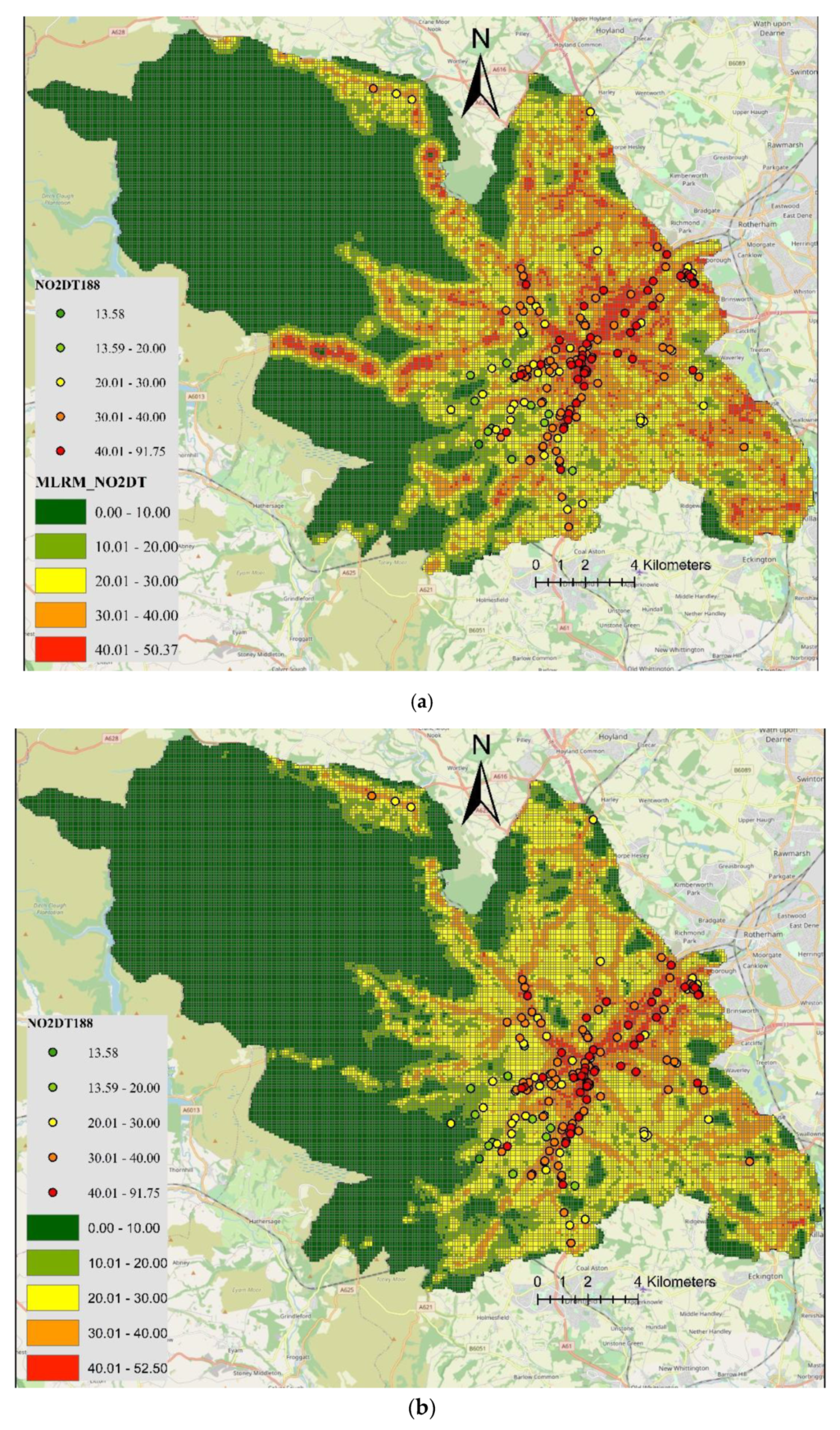
Furthermore, NO2 concentration was predicted for 37,605 square grids with 100 m × 100 m resolution to produce maps of NO2 concentrations for the entire Sheffield City. The resultant maps of predicted NO2 concentrations for both MLRM and GAM are shown in Figure 5. The model successfully captured spatial variability of NO2 concentrations in Sheffield, showing higher levels of NO2 in the city centre and on busy roads around the city. The city centre and the area between the motorway (M1) and the city centre is particularly highlighted with NO2 levels higher than EU annual limits of 40 µg/m3 (Figure 5). Western part of the city especially Peak District National Park has shown lower level of NO2 concentrations due to high altitude and limited amount of minor and major roads. Recently, Munir et al. [21] using Airviro dispersion modelling system, have reported similar results in Sheffield. However, the results of this study are much more detailed (100 m × 100 m resolution), successfully capturing micro-level local variations in NO2 concentrations, intended for quantifying public exposure. The maps show how NO2 levels vary from street to street. Spatial trends of predicted NO2 levels closely match with measured NO2 levels (Figure 5).

3.2. LUR Model Using NO2 Data from LCS

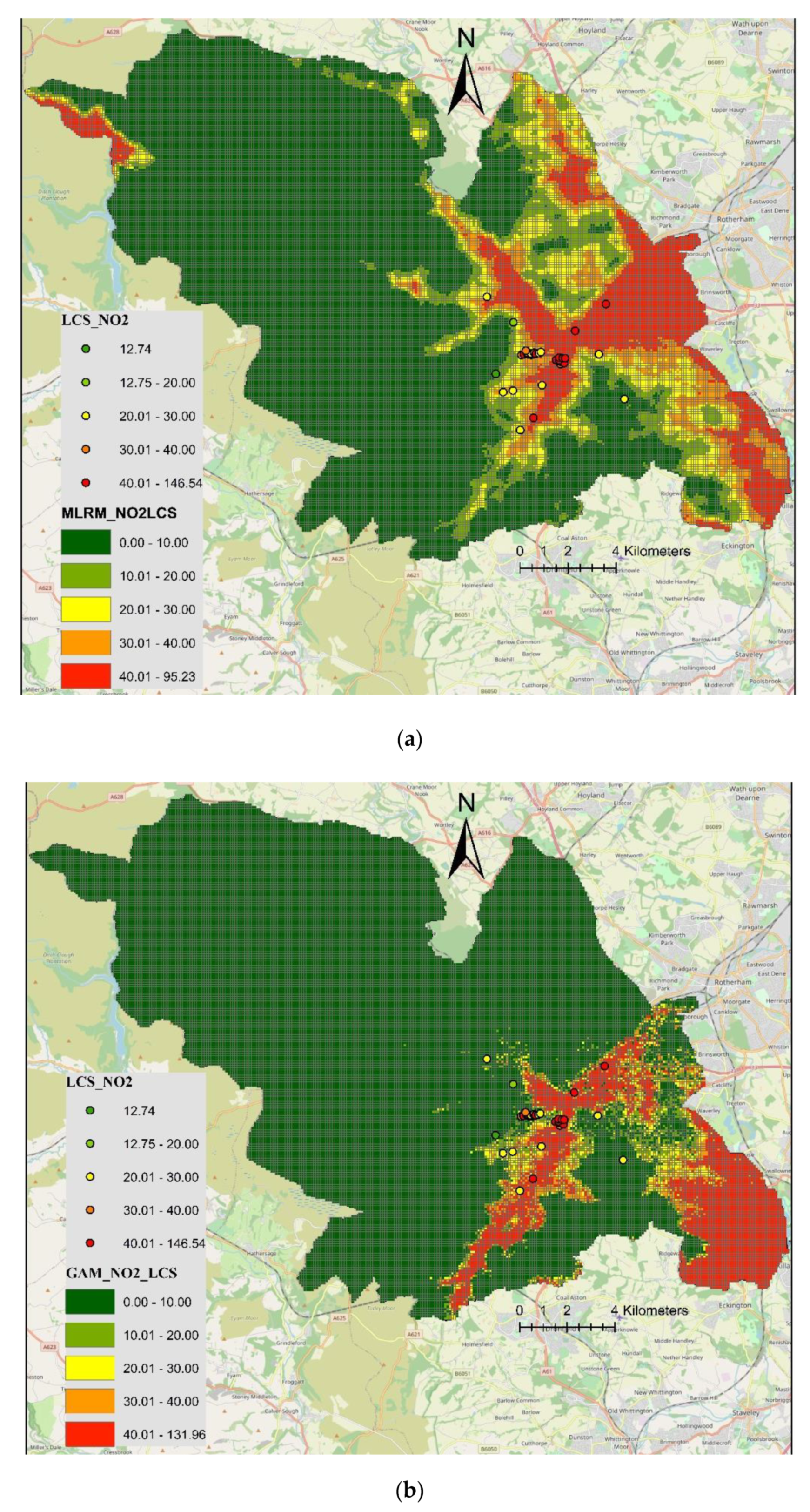
Employing MLRM and GAM, NO2 concentration (µg/m3) from 40 LCS was modelled using the same predictor variables as in Section 3.1. Using a stepwise regression algorithm 5-covairaites were found to have a significant effect on NO2 concentrations, which were: distance to major road, distance to minor road, distance to commercial area, distance to residential area, and altitude. Several statistical metrics for both fitted and cross validated models are shown in Table 4. Comparing fitted model, GAM with r-value of 0.89 showed better performance than the MLRM with r-value 0.55. However, when the models were applied to an independent set of data (hold-out dataset), MLRM showed better performance (r-value = 0.78) as compared to GAM (r-value = 0.56). Likewise, metrics (e.g., RMSE, MGE, NMGE, NMB) showing error of the models were lower for training dataset and higher for testing dataset for GAM than MLRM. FAC2 having value of 1 or nearly 1 shows acceptable model performance for both MLRM and GAM. The results of MLRM on hold-out dataset do not seem genuine as r-value is greater and RMSE is less than the fitted model, which probably shows that the model is over-fitted. This is also confirmed by the fact that overall both fitted and cross-validated model showed good performance, however, when the model results were extrapolated to the entire city, both MLRM and GAM models failed to predict the expected spatial variability of NO2 concentrations in the city (Figure 6), which should have been more like Figure 5. This is probably due to the fact that LCS are mostly installed in the city centre and at the University of Sheffield, and are not representing the wider area of the city. Therefore, extrapolation of the modelled NO2 outside the calibration range, results in unreasonable values. Secondly, there were only 40 LCS probably not providing enough spatial coverage to represent the whole city. Therefore, the models are over fitted and are not successfully fitting the data from the rest of the city.
Gillespie et al. [18] developed an LUR model to estimate exposure to NO2 in Glasgow, Scotland. They used 135 NO2 passive diffusion tubes, which were divided to four groups (32–35 sites per group) and models were developed using a combination of 1 to 3 groups as training sites to assess how the number of training sites affected the model performance. The explanatory variables used in the models were major road length, minor road length, all urban areas, building volume, distance to nearest major or minor road, green rural area, minor road length, and street configuration. The models were able to explain moderate to high variance in the data, where R2 ranged from 0.62 to 0.89 for training dataset and 0.44 to 0.85 for hold-out dataset. Precision of estimated exposure was increased with increasing number of training sites. Gillespie et al. [16] concluded that the use of more than 60 training sites in LUR model has quantifiable benefits in epidemiological application. Therefore, this might suggest that probably in present study the number of sites (40 LCS) were not enough and resulted in over fitting of the model.

3.3. LUR Model Using NO2 Data from DT and LCS

In this section NO2 data from 188 DT and 40 LCS were combined to increase the number of monitoring sites and see how it affects the model outputs. At the model selection stage six predictors showed significant effect, which were distance to major road, minor roads length, commercial area, population, distance to commercial area and altitude. Performance of the model was assessed by calculating several statistical metrics as shown in Table 5. In case of MLRM, r-values were 0.60 and 0.52 for training and hold-out dataset, whereas in case of GAM r-values were 0.69 and 0.53, respectively. Metrics (e.g., RMSE, MGE, NMGE, MB and NMB) expressing error of the models have smaller values for GAM than MLRM, showing GAM outperforms MLRM. FAC2 also shows that prediction of GAM is closer to the measured values. Furthermore, comparing Table 5 with Table 3, it can be clearly observed that combining DT and LCS did not improve the models performance compared to the models using DT data only. This is probably due to the fact that DT and LCS use different techniques for measuring NO2 concentrations and combining their data might not be the right thing to do. Second, DT provide long-term NO2 concentrations (e.g., annual mean), whereas LCS provide short-term average (e.g., 5 min to 1 h mean), which is converted to annual mean. It probably indicates that ideally all sensors should be of the same type and mixing of sensors of different grades might cause conflict and affect the model outputs. Finally, 188 DT are enough to build an LUR model, further increasing the number does not improve the model outputs.
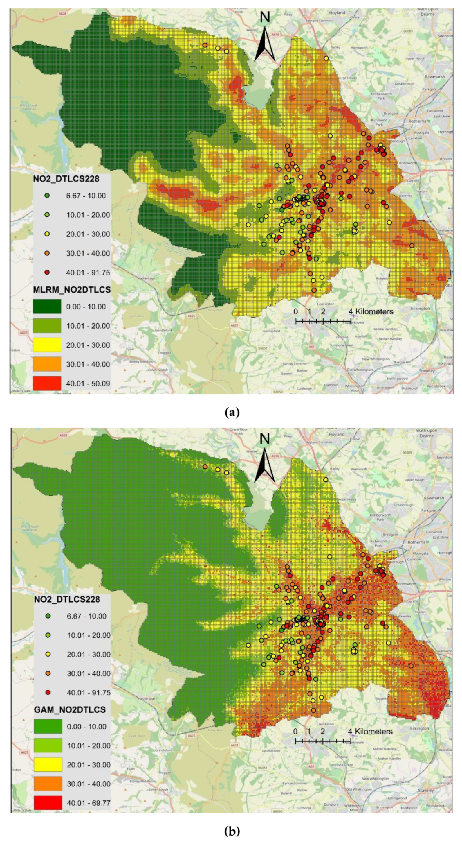
Figure 7 shows the maps of predicted NO2 concentrations, where NO2 concentrations predicted by MLRM range from 0 to 50 µg/m3, whereas NO2 concentrations predicted by GAM range from 0 to 70 µg/m3. City centre and the eastern side of the city towards the motorway are highlighted as having high levels of NO2 due to lower altitude and greater length of major and minor roads and commercial areas.
Major roads, minor roads, commercial areas and altitude had significant effects in all three models (described in Section 3.1, Section 3.2 and Section 3.3). Residential areas had significant effect in two models, whereas bus stops and population had significant effect only in one model. This shows that in addition to emission sources, topography especially altitude plays an important role in controlling the levels of air pollution. However, the effect of predictor variables is not the same everywhere and may change from region to region. To build an LUR model, researchers have used different sets of land use and traffic related features. The most common predictor variables used are topography, land use, traffic, population density, altitude and meteorological parameters. The use of these variables in the regression model are known to capture small scale variability [17]. The effect of predictor variables may vary from one area to another, depending on the nature of geographical conditions, size of urban area, the type of environment of the monitoring site (e.g., roadside, urban background or rural) and type of the pollutant modelled (e.g., NO2, O3, VOCs, PM10, PM2.5 etc.). The main constraint for building an LUR model is the unavailability of reasonable size monitoring network to provide measured data of pollutant for fitting and validating the model. This is particularly a problem in poor and low income countries having no air quality monitoring networks. To overcome this problem, Molter et al. [32] have suggested to use existing data from a dispersion air quality model. However, this is a problem in itself as dispersion model requires emission, geographical and meteorological data.
To the best of our knowledge, almost all previous investigations have used linear regression approach for building LUR model. Therefore, linear regression has become a default methodology for developing LUR models. This is due to the fact that in contrast to linear regressions, nonlinear regressions do not produce a single coefficient for each explanatory variable and therefore need to be applied in a different way to the traditional linear methods. With advances in IT and data analysis software (e.g., R programming language and Python), nonlinear LUR models can be developed and predicted in these software. These software have several special packages for spatial analysis and producing maps of measured or predicted pollutants. Therefore, maps of the predicted pollutants can be either produced in these software or alternatively the predicted pollutants can be exported to GIS software (e.g., ArcGIS) for further analysis. In this paper, the nonlinear model was developed using both R programming language and ArcGIS. The proposed method provides a basis for further application of advanced nonlinear modelling approaches to constructing LUR models in urban areas which enable quantifying small scale variability in pollution levels.

4. Conclusions

It has been a common practice to use the linear regression for developing LUR models, however, the association between air pollutant levels and spatial features is not always linear, therefore, ideally nonlinear modelling approaches should be used for developing LUR models, which can help in understanding small scale spatial variability of different air pollutants in urban areas. In this paper, the GAM was fitted and predicted in R programming language and the predicted concentrations was then transferred to ArcGIS for producing maps of NO2 in Sheffield. Alternatively, R has several special packages that can be used for mapping and spatial analysis of the predicted concentrations.
In this paper spatial variability of NO2 concentration is modelled in the city of Sheffield for year 2019. MLRM is a traditional and most commonly used approach for developing LUR models, here in addition to the linear approach, a nonlinear GAM model is employed and its benefits and the way it is applied are discussed. Three datasets of NO2 measurements were used: (a) NO2 data from 188 DT, (b) NO2 from 40 LCS, and (c) NO2 data from both DT and LCS. The first group performed better than the other two groups. Among predictor variables altitude (negative effect), major roads (positive effect), minor roads (positive effect), and commercial area (positive effect) had significant effect in all three groups. The model successfully captured the spatial variability of NO2 in Sheffield, estimating high levels of NO2 in the city centre and on major roads around the city. The eastern area between the city centre and motorway (M1) showed particularly high levels, whereas the western area (Peak District National Park) demonstrated lower levels of NO2 concentrations.
The main contributions of this work are summarised as follows: (a) An advanced nonlinear GAM is proposed for developing an LUR model, which outperforms the linear counterpart. (b) High resolution maps (100 m × 100 m) of NO2 are developed in Sheffield using a nonlinear LUR model for quantifying public exposure to NO2 and determining how the exposure varies at small scales in the city. (c) NO2 data measured by a network of DT and LCS are integrated to developed high resolution maps. (d) It is confirmed that Sheffield City Centre and its eastern sides experience relatively higher levels of NO2 pollution.
Future work could include developing a spatiotemporal LUR model using meteorology, traffic counts and fleet composition data. In this study, the effect of major and minor roads is analysed on NO2 levels, however, road traffic and composition may vary from time to time on a given road. It is, therefore, important to capture temporal and spatial variability in meteorology and traffic data and feed it to the nonlinear LUR models. This will probably further improve the model performance, depending on the quality and temporal resolution of the data.

Author Contributions

S.M., M.M. and D.C. planned and designed the original idea. S.M. obtained the data and did the modelling. M.M. and D.C. won the funding for this research project. S.M. wrote the first draft of the manuscript under the supervision of M.M. and D.C. L.S.M., M.M. and D.C. reviewed and edited the manuscript. All the authors have read and approved the content of the manuscript. All authors have read and agreed to the published version of the manuscript.

Funding

This research was funded by the Engineering and Physical Sciences Research Council (EPSRC) (grant number - EP/R512175/1) and Siemens plc. The APC was paid by UKRI/EPSRC.

Acknowledgments

We would like to express our thanks to the Engineering and Physical Sciences Research Council (EPSRC), grant number - EP/R512175/1 and Siemens plc for funding this project. We are also thankful to Sheffield City Council for providing NO2 diffusion tubes data.

Conflicts of Interest

All the authors declare no conflict of interest.

References

  1. Landrigan, P.J. Air pollution and health. Lancet Public Health 2016, 2, E4–E5. [Google Scholar] [CrossRef] [Green Version]
  2. WHO. Review of Evidence on Health Aspects of Air Pollution-REVIHAAP Project: Final Technical Report. World Health Organziation Regional Office for Europe, 2013. Available online: http://www.euro.who.int/en/health-topics/environment-and-health/airquality/publications/2013/review-of-evidence-on-health-aspects-of-air-pollutionrevihaap-project-final-technical-report (accessed on 12 February 2020).
  3. DEFRA. Improving Air Quality in the UK Tackling Nitrogen Dioxide in Our Towns and Cities, UK Overview Document. December 2015. Available online: https://www.gov.uk/government/uploads/system/uploads/attachment_data/file/486636/aq-plan-2015-overview-document.pdf (accessed on 9 April 2020).
  4. Hsu, S.; Mavrogianni, A.; Hamilton, I. Comparing spatial interpolation techniques of local urban temperature for heat-related health risk estimation in a subtropical city. Procedia Eng. 2017, 198, 354–365. [Google Scholar] [CrossRef]
  5. Briggs, D.J. The Role of Gis: Coping with Space (And Time) in Air Pollution Exposure Assessment. J. Toxicol. Environ. Health Part A 2005, 68, 1243–1261. [Google Scholar] [CrossRef] [PubMed]
  6. Schneider, P.; Castell, N.; Vogt, M.; Dauge, F.R.; Lahoz, W.A.; Bartonova, A. Mapping urban air quality in near real-time using observations from lowcost sensors and model information. Environ. Int. 2017, 106, 234–247. [Google Scholar] [CrossRef] [PubMed]
  7. Briggs, D.J.; De Hough, C.; Gulliver, J.; Wills, J.; Elliott, P.; Kingham, S.; Smallbone, K. A regression-based method for mapping traffic-related air pollution: Application and testing in four contrasting urban environments. Sci. Total Environ. 2000, 253, 151–167. [Google Scholar] [CrossRef]
  8. Hoek, G.; Beelen, R.; De Hoogh, K.; Vienneau, D.; Gulliver, J.; Fischer, P.; Briggs, D. A review of land-use regression models to assess spatial variation of outdoor air pollution. Atmos. Environ. 2008, 42, 7561–7578. [Google Scholar] [CrossRef]
  9. Briggs, D.J.; Collins, S.; Elliott, P.; Fischer, P.; Kingham, S.; Erik Lebret, K.P.; Van Reeuwijk, H.; Smallbone, K.; Van der Veen, A. Mapping urban air pollution using GIS: A regression-based approach. Int. J. Geogr. Inf. Sci. 1997, 11, 699–718. [Google Scholar] [CrossRef] [Green Version]
  10. Eeftens, M.; Beelen, R.; De Hoogh, K.; Bellander, T.; Cesaroni, G.; Cirach, M.; Declercq, C.; Dėdelė, A.; Dons, E.; De Nazelle, A.; et al. Development of land use regression models for PM2.5, PM2.5 absorbance, PM10 and PM coarse in 20 European Study areas; results of the ESCAPE project. Environ. Sci. Technol. 2012, 46, 11195–11205. [Google Scholar] [CrossRef]
  11. Lee, J.H.; Wu, C.F.; Hoek, G.; Hoogh, K.; Beelen, R.; Brunekreef, B.; Chan, C.-C. Land use regression models for estimating individual NOx and NO2 exposures in a metropolis with a high density of traffic roads and population. Sci. Total Environ. 2013, 472, 1163–1171. [Google Scholar] [CrossRef] [PubMed]
  12. Muttoo, S.; Ramsay, L.; Brunekreef, B.; Beelen, R.; Meliefste, K.; Naidoo, R.N. Land use regression modelling estimating nitrogen oxides exposure in industrial south Durban, South Africa. Sci. Total Environ. 2017, 610–611, 1439–1447. [Google Scholar] [CrossRef]
  13. Rahman, M.M.; Yeganeh, B.; Clifford, S.; Knibbs, L.D.; Morawska, L. Development of a land use regression model for daily NO2 and NOx concentrations in the Brisbane metropolitan area, Australia. Environ. Model. Softw. 2017, 95, 168–179. [Google Scholar] [CrossRef] [Green Version]
  14. Stedman, J.; Vincent, K.; Campbell, G.; Goodwin, J.; Downing, C. New high resolution maps of estimated background ambient NOx and NO2 concentrations in the U.K. Atmos. Environ. 1997, 31, 3591–3602. [Google Scholar] [CrossRef]
  15. Beelen, R.; Hoek, G.; Fischer, P.; Van den Brandt, P.A.; Brunekreef, B. Estimated long-term outdoor air pollution concentrations in a cohort study. Atmos. Environ. 2007, 41, 1343–1358. [Google Scholar] [CrossRef]
  16. Ryan, P.H.; LeMasters, G.K.; Biswas, P.; Levin, L.; Hu, S.; Lindsey, M.; Bernstein, D.I.; Lockey, J.; Villareal, M.; Hershey, G.K.K.; et al. A comparison of proximity and land use regression traffic exposure models and wheezing in infants. Environ. Health Perspect. 2007, 115, 278–284. [Google Scholar] [CrossRef] [Green Version]
  17. Ryan, P.H.; LeMasters, G.K. A review of land-use regressionmodels for characterizing intraurban air pollution exposure. Inhal. Toxicol. 2007, 19 (Suppl. 1), 127–133. [Google Scholar] [CrossRef] [Green Version]
  18. Gillespie, J.; Beverland, I.J.; Hamilton, S.; Padmanabhan, S. Development, Evaluation, and Comparison of Land Use Regression Modeling Methods to Estimate Residential Exposure to Nitrogen Dioxide in a Cohort Study. Environ. Sci. Technol. 2016, 50, 11085–11093. [Google Scholar] [CrossRef] [PubMed] [Green Version]
  19. Beelen, R.; Hoek, G.; Vienneau, D.; Eeftens, M.; Dimakopoulou, K.; Pedeli, X.; Tsai, M.Y. Development of NO2 and NOx land use regression models for estimating air pollution exposure in 36 study areas in Europe e-The ESCAPE project. Atmos. Environ. 2013, 72, 10–23. [Google Scholar] [CrossRef]
  20. Vienneau, D.; De Hoogh, K.; Beelen, R.; Fischer, P.; Hoek, G.; Briggs, D. Comparison of land-use regression models between Great Britain and the Netherlands. Atmos. Environ. 2010, 44, 688–696. [Google Scholar] [CrossRef]
  21. Munir, S.; Mayfield, M.; Coca, D.; Mihaylova, L.S.; Osammor, O. Analysis of air pollution in urban areas with Airviro dispersion—A Case Study in the City of Sheffield, United Kingdom. Atmosphere 2020, 11, 285. [Google Scholar] [CrossRef] [Green Version]
  22. Munir, S.; Mayfield, M.; Coca, D.; Jubb, S.A. Structuring an Integrated Air Quality Monitoring Nework in Large Urban Areas—Discussing the Purpose, Criteria and Deployment Strategy. Atmos. Environ. X 2019, 2, 100027. [Google Scholar]
  23. R Core Team. R: A Language and Environment for Statistical Computing; R Foundation for Statistical Computing: Vienna, Austria, 2019; Available online: https://www.R-project.org/.
  24. Wood, S.N.; Augustin, N.H. GAMs with integrated model selection using penalized regression splines and applications to environmental modelling. Ecol. Model. 2002, 157, 157–177. [Google Scholar] [CrossRef] [Green Version]
  25. Wood, S.N. Fast stable restricted maximum likelihood and marginal likelihood estimation of semiparametric generalized linear models. J. R. Stat. Soc. B 2011, 73, 3–36. [Google Scholar] [CrossRef] [Green Version]
  26. Wood, S.N. Generalized Additive Models: An Introduction with R 2006; Chapman and Hall: London, UK; CRC Press: Boca Raton, FL, USA, 2006. [Google Scholar]
  27. Hastie, T.J.; Tibshirani, R.J. Generalised Additive Models 1990; Chapman and Hall: London, UK, 1990. [Google Scholar]
  28. Venables, W.N.; Ripley, B.D. Modern Applied Statistics with S, 4th ed.; Springer: New York, NY, USA, 2002; ISBN 0-387-95457-0. [Google Scholar]
  29. Carslaw, D.C.; Ropkins, K. Openair—An R package for air quality data analysis. Environ. Model. Softw. 2012, 27–28, 52–61. [Google Scholar] [CrossRef]
  30. Korek, M.; Johansson, C.; Svensson, N.; Lind, T.; Beelen, R.; Hoek, G.; Pershagen, G.; Bellander, T. Can dispersion modeling of air pollution be improved by land-use regression? An example from Stockholm, Sweden. J. Expo. Sci. Environ. Epidemiol. 2017, 27, 575–581. [Google Scholar] [CrossRef] [Green Version]
  31. Ji, H.; Chen, S.; Zhang, Y.; Chen, H.; Guo, P.; Zhao, P. Comparison of air quality at different altitudes from multi-platform measurements in Beijing. Atmos. Chem. Phys. 2018, 18, 10645–10653. [Google Scholar] [CrossRef] [Green Version]
  32. Molter, A.; Lindley, S.; De Vocht, F.; Simpson, A.; Agius, R. Modelling air pollution for epidemiologic research—Part I: A novel approach combining land use regression and air dispersion. Sci. Total Environ. 2010, 408, 5862–5869. [Google Scholar] [CrossRef]
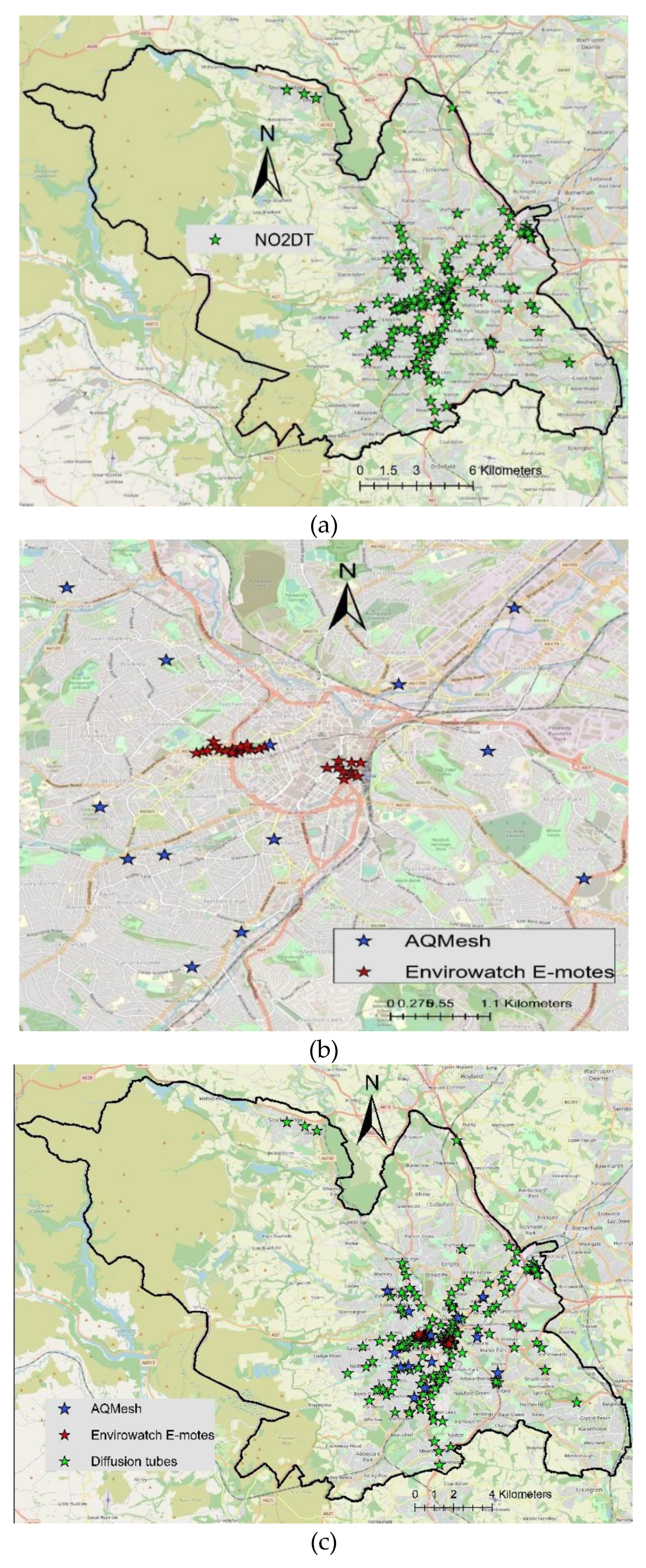
Figure 1. (a) Showing the locations of 188 NO2 diffusion tubes (DT), (b) 40 low-cost sensors (LCS): 13 AQMesh pods and 27 Envirowatch E-motes, and (c) both LCS and DT in the City of Sheffield.
Atmosphere 11 00736 g001
Figure 2. (a) Altitude, (b) major roads, commercial and residential area (c) and motorway, green parks and industrial area in Sheffield.
Atmosphere 11 00736 g002
Figure 3. (a) Showing the nonlinear association of NO2 concentrations (µg/m3) with altitude in meters and (b) distance to major roads in meters. The dashed lines are the estimated 95% confidence intervals. The vertical lines on the x-axis show the presence of data.
Atmosphere 11 00736 g003
Figure 4. (a,b) Comparing measured and predicted NO2 concentrations using multiple linear regression model (MLRM) and generalised additive model (GAM) for training (c,d) and testing dataset using NO2 data from diffusion tubes (DT) only.
Atmosphere 11 00736 g004
Figure 5. High resolution maps (100 m × 100 m) of NO2 concentrations (µg/m3) predicted by (a) MLRM and (b) GAM in Sheffield. The points show values of NO2 measured by DT.
Atmosphere 11 00736 g005
Figure 6. High resolution (100 m × 100 m) maps of NO2 concentrations (µg/m3) in Sheffield, predicted by (a) MLRM and (b) GAM. The points show values of NO2 measured by LCS.
Atmosphere 11 00736 g006
Figure 7. High resolution (100 m × 100 m) maps of predicted NO2 concentrations (µg/m3) in Sheffield, estimated by (a) MLRM, and (b) GAM. The points show values of NO2 measured by both DT and LCS.
Atmosphere 11 00736 g007
Table 1. Descriptive statistics of NO2 measured by DT (diffusion tubes) and LCS (low-cost sensors) in Sheffield.
MetricsDT NO2LCS NO2
Minimum13.5812.74
1st Quartile (25th percentile)28.2925.23
Median33.7733.19
Mean34.2341.23
3rd Quartile (75th percentile)40.0045.28
Maximum62.03146.54
Standard Deviation9.6527.69
Table 2. Showing coefficients and significance levels of different predictor variables for MLRM (multiple linear regression models).
Predictor VariableCoefficientp-Value
Intercept43.7025<2 × 10⁻¹⁶ ***
Building0.00200.075 +
Dist_MajorRd−0.01140.001 **
Dist_MinorRd−0.09680.052 +
Residential−0.00060.002 **
Commercial0.00050.053 +
Altitude−0.05430.000 ***
Dist_Bstop−0.03080.026 *
Note: p.stars relate to how statistically significant the effect is: p-value <0.001 = ∗∗∗, p-value <0.01 = ∗∗, p-value <0.05 = ∗ and p-value <0.1 = +.
Table 3. Showing various statistical metrics for assessing the performance of MLRM and GAM for both fitted model (FM) using training dataset and cross-validated model (CV) using hold-out dataset based on NO2 data from DT. MB (mean bias), MGE (mean gross error) and RMSE (root mean square error) have the same units as the quantity being considered (here µg/m3), whereas FAC2, r, NMGE and NMB are unitless.
MetricsMLRMGAM
FMCVFMCV
FAC21111
MB2 × 10−15−0.952 × 10⁻¹¹−1.17
MGE4.986.894.806.55
NMB2 × 10−17−0.032 × 10⁻¹²−0.03
NMGE0.150.190.140.18
RMSE6.448.986.138.69
r0.670.670.730.70
Table 4. Showing various statistical metrics for assessing the performance of MLRM and GAM for both fitted model (FM) using training dataset and cross-validation (CV) using hold-out dataset based on NO2 data from LCS.
MetricsMLRMGAM
FMCVFMCV
FAC20.97110.90
MB2 × 10−15−0.482 × 10⁻¹⁰−3.76
MGE11.078.827.6016.35
NMB2 × 10−16−0.012 × 10⁻¹²−0.10
NMGE0.290.240.200.44
RMSE19.3112.5610.4022.21
r0.550.780.890.56
Table 5. Showing various statistical metrics for assessing the performance of the MLRM and GAM for both fitted model (FM) using training dataset and cross-validation (CV) using hold-out dataset based on NO2 data obtained from DT and LCS.
MetricsMLRMGAM
FMCVFMCV
FAC20.930.890.990.91
MB2 × 10−15−2.28−4.01−2.03
MGE7.319.326.499.21
NMB2 × 10−16−0.09−1.28−0.07
NMGE0.230.310.210.30
RMSE9.4712.338.6212.22
r0.600.520.690.53