Abstract
An intensity modulated, continuous-wave (IM-CW) integrated path differential absorption (IPDA) fiber-based lidar is developed herein for measuring atmospheric carbon dioxide (CO2). There are two main challenges in improving measurement accuracy, which have not been given enough attention in the previous research: one is that temperature sensitivity in optical components causes biases, due to the drift of component characteristic, and the other is that speckle noise deteriorates the signal-to-noise ratio. With the components thermally controlled, a target calibration accuracy of 0.003 dB is realized, corresponding to a CO2 concentration precision of better than 1 ppm for a 1 km path. A moving diffuser can reduce speckle noise by time averaging. In this paper, movement of the diffuser is substituted by the perturbation of the emitted laser beam by using a vibrating motor mounted on the optical antenna. Selecting on and off wavelengths with a small wavelength separation can improve the correlation between two laser speckle fields. These improvements result in the improved accuracy of the IPDA lidar system. Finally, the lidar performance was analyzed after the improvements described above were implemented. The diurnal variations of the atmospheric CO2 concentration using a topographic target were performed, and the results showed good agreement with the data measured by an in situ sensor. The root mean square (rms) of the deviation between the IPDA lidar and the in situ sensor was less than 1.4%.
1. Introduction
Atmospheric CO2 is presently regarded as the largest anthropogenic forcing factor for climate change, but the global CO2 budget remains considerably uncertain [1,2]. To be useful in reducing uncertainties about carbon sources and sinks, atmospheric CO2 measurements need to have a high resolution, with 1% precision [3]. To meet this need, differential absorption lidar (DIAL) or laser absorption spectrometer (LAS) systems, which use conventional coherent or incoherent lidar methods, have recently been developed.
Many publications have reported the successful measurement of the atmospheric CO2 column or profile concentrations by ground-based or airborne instruments using laser transmitters at wavelengths of near 2.0 μm or 1.57 μm. Koch et al. and Gibert et al. demonstrated a range-resolved backscatter CO2 profiling lidar using a line near 2.0 μm, a pulsed Ho:Tm:YLF laser, and a coherent receiver [4,5,6,7]. However, the detected power fluctuated obviously, due to the speckle effects in these systems. This is quite a serious problem, as it implies that a large number of pulses are necessary to obtain signals with a stable intensity [8]. Amediek et al. reported an integrated path differential absorption (IPDA) lidar operating at 1.57 μm using direct-detection, where an injection seeded KTP -OPO system pumped by an Nd:YAG laser serves as the transmitter [9]. Comparative measurements on diurnal CO2 variations performed by this lidar and an in situ device showed good agreement, but the maximum deviation was 9% (rms). Abshire et al. reported on airborne CO2 column absorption measurements with a pulsed direct-detection multi-wavelength IPDA lidar operating at 1572.33 nm [10]. In all the pulsed lidar systems mentioned above, the on and off lasers are separated in time or space. Consequently, the sensing columns and footprints of the laser beam are different, which will introduce measurement errors, especially in space applications [8].
Recently, a continuous laser DIAL system with fiber transmission has been developed, which presents advantages compared with the scheme of a pulsed laser propagating in free space, such as continuous laser tenability and compactness. Another attractive feature of this technology is that the fiber interconnects allow for the straightforward development of system configurations [11]. Dobler et al. developed an intensity modulated, continuous-wave (IM-CW) LAS system by using the backscatter from a geometric target, and which operated at a wavelength of 1.6 μm [12]. Diode lasers operating at discrete on and off wavelengths are intensity modulated at different frequencies, as well as combined and amplified simultaneously in a single erbium-doped fiber amplifier (EDFA). This instrument has been successfully flight tested in many airborne campaigns conducted in different geographic regions over the past few years [13,14,15,16]. They improved their system by using a swept modulation frequency technique to provide range discrimination, due to the ubiquitous nature of cirrus clouds for space applications, and achieved a very high accuracy: the contrast error between the lidar and in situ CO2 measurements was less than 0.6%. They found that the CO2 measurement precision improved considerably after transitioning to the more thermally controlled cabin environment associated with the aircraft [14]. However, details about the influence of the cabin’s ambient temperature on system errors was not reported in their reports. Kameyama et al. developed a dual-wavelength IM-CW IPDA lidar for CO2 measurements at the CO2 absorption line near 1.6 μm, where the transmitting and monitoring beams were all in fibers [17]. They added a horizontal rotator and vibrator on the optical antenna unit to average the speckle patterns which were independent between two wavelengths. The monitoring photodetector was thermoelectric cooled to maintain the etalon characteristics in the detector. They reported ground-based CO2 absorption measurements over a 1 km long horizontal path with 4 ppm fluctuations after the system was improved [18].
With the more accurate absorption line information (2% to 5% uncertainty) in the HITRAN database and the development of photodetectors and frequency-locked narrow linewidth lasers, these parameters (i.e., absorption line information, detector noise, wavelength accuracy, stability and spectral purity) are not the main factors limiting the near-ground horizontal path measurement accuracy of a 1.57 μm IPDA lidar any more [19,20]. However, some potential sources of uncertainty remain, which may arise from the temperature sensitivity of the optical components in an optical fiber transmission system without calibration [18]. In addition, speckle appears when a laser is scattered by heterogeneities at the scale of its wavelength, such as variations in the surface roughness, or in the refractive index caused by atmospheric turbulence [21]. Speckle fluctuation leads to a large uncertainty in detected powers unless the signal is averaged over many independent speckle patterns. Kameyama et al. have revealed the temperature-dependent characteristics of optical components and the speckle effect, which have an impact on the measurement accuracy in their IM-CW IPDA lidar. These phenomena also appeared in our experiments, indicating that they are ubiquitous in IM-CW IPDA fiber transmission lidar systems.
In a previous study, we developed a 1.57 μm IM-CW IPDA lidar system for CO2 sensing, with which the transmitted optical signals are backscattered from a random topographic target [20]. In this paper, we verified the effectiveness of the lidar calibration process reported by Kameyama et al. on our system and presented the improvement of speckle statistics. An optical fiber link test (OFLT) unit is designed to locate the temperature-dependent optical components that cause the bias drift of our lidar system, and the calibration of the OFLT is completed. Then, we demonstrate, using theoretical and modeling techniques, that there is a substantial advantage (in terms of the variance of the ratio of return powers) for a highly correlated speckle. A theoretical prediction is that placing a vibrating motor on the telescope to perturb the emitted beam and reduce the wavelength separation between the on and off wavelengths will increase the correlation of speckle. The results of laboratory experiments are consistent with the theoretical prediction. This paper is structured as follows: Section 2 introduces the principle of IPDA lidar and the preliminary instrument setup. The process of system calibration and the theoretical analysis of speckle statistics are discussed in Section 3. In Section 4, the verification experiment of improved speckle statistics is introduced and the results of the CO2 concentration measurement using the improved lidar system are shown. Section 5 summarizes the most important findings and describes the limitations of this study.
2. Theory and Experimental Instrument
2.1. Measurement Principle
Dual-wavelength IPDA lidar systems, presented in this study, consist of two continuous wave seed lasers. One wavelength is tuned onto or near the center of an absorption line, denoted as the on wavelength, and a reference off wavelength is used with significantly less absorption. For simplicity, the lidar equation for the received signal power at wavelength , from a scattering target at range R, is given by [22]:
where is the integral path, is the laser emission power, is the optical efficiency of the system, is the target reflectivity, is the effective receiving area, is the dry air volume mixing ratio of CO2, is the volume mixing ratio of water vapor, is the air number density, and is the absorption cross-section. Knowledge of the water vapor mixing ratio is necessary in order to derive the dry air mixing ratio of CO2. For a DIAL that uses on and off wavelengths which are very close together (<0.2 nm), differences in the reflectivity, backscatter coefficients, and the absorption of other molecules are negligible. By taking the ratio of the two simultaneous measurements, and assuming that the instrument is designed properly such that the receiver dependent differences at the two wavelengths are either negligible or constant and well calibrated, one arrives at the standard DIAL equation:
The column-averaged dry air CO2 mixing ratio () is given by [23]:
where is the dry air number density, and the differential absorption cross-section is given by .
2.2. Preliminary Configuration and Results
The preliminary system configuration for the first trial of CO2 sensing is shown in Figure 1 and the main system parameters are listed in Table 1. The on light was tapped by the splitter, and the 30% portion was used to lock the wavelength at the absorption peak of the CO2 gas cell, based on the frequency modulation spectroscopy. The off light and 70% of the on light were intensity modulated with CW signals at slightly different frequencies (e.g., 99.7 kHz and 101.8 kHz in Figure 1), in order to distinguish the received on and off radiation. The modulated lights were amplified by an erbium-doped fiber amplifier (EDFA) after being combined with an optical coupler. The polarization state of the on and off light output from the single-mode (SM) EDFA was uncertain, so we used a polarization-insensitive SM filter beam splitter, instead of a fused SM fiber beam splitter, to split the output beam of the EDFA into 99% and 1% [18]. The 99% portion was transmitted to a hard-target and the 1% portion was detected by the photodetector for transmission monitoring. The monitored and received signals were analog-to-digital (A/D) converted and their spectrum information was obtained by the fast Fourier transform (FFT). The intensities of two peaks in the spectrum of the received signal were normalized by the monitored signal. The differential absorption optical depth (DAOD) was obtained using the logarithm of the normalized detected intensities ratio of the two wavelengths, as shown in Equation (2). The ranging of the hard-target was possible by utilizing the phase difference between the monitored and the received signal. Because CW signals were used for this ranging, there was folding ambiguity [24]. A priori information on the range—i.e., if the information has the precision of ≪c/(2fm), where c is the speed of light and fm is the modulation frequency—solves this problem. This precision can be easily obtained in ground-based measurements if the modulation frequency is lower than or equal to the 100 kHz band [18].
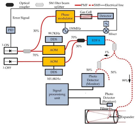
Figure 1.
The system configuration for the first trial. PMF, polarization maintaining fiber; SMF, single-mode fiber; DDS, direct digital synthesis; PID, proportional-integral-differential control system; AOM, acoustic-optic modulator; EDFA, erbium-doped fiber amplifier.

Table 1.
Primary parameters of the 1.57 μm intensity modulated, continuous-wave (IM-CW) integrated path differential absorption (IPDA) lidar system.
The CO2 concentration measurement results, with a short measurement interval of 30 s during the first CO2 sensing trial with the system configuration shown in Figure 1 on a 1.5 km horizontal path, are shown in Figure 2. The open-path is located in Hongkou District, Shanghai, China, and the measurement date is 14 September 2019. Figure 2a shows the carrier-to-noise ratios (CNRs) of the receiving and monitoring signals for both the on and off wavelengths. The signal-to-noise ratios (SNRs) of the receiving and monitoring signals are equal to the CNRs, if no speckle-related noise appears. By using these CNRs, we calculated that the random error in the CO2 concentration was less than 0.1 ppm. However, the random error of the preliminary experiment, as shown in Figure 2c, far exceeded this calculated value. Speckle noise may have been the main reason for poor SNRs. It can be seen from Figure 2b that the random error of path length measurements was 2 m and the drift over a long time was 1 m. The drift of the CO2 concentration corresponding to the path length drift was less than 0.27 ppm. In the first trial, the detected CO2 mixing ratio strongly fluctuated around the expected 410 ppm ambient concentration, with minimum and maximum values of 300 and 600 ppm, respectively. Therefore, it was believed that unknown sources of systematic errors caused large fluctuations in the CO2 concentration, indicating the necessity for a system calibration.
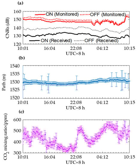
Figure 2.
(a) The carrier-to-noise ratio (CNRs) of the receiving and monitoring signals for both the on and off wavelengths; (b) the path length; and (c) the CO2 concentration in Shanghai city for one day during the first trial.
3. Calibration System and Improved Speckle Statistics
3.1. System Errors Sources
Systematic errors of the IM-CW IPDA lidar may arise for different reasons: (i) uncertainty in temperature and pressure measurements, (ii) frequency stability of the on wavelength and the linewidth of laser, (iii) influence of gases other than CO2, and (iv) the drift of optical component characteristics. For (i), the HITRAN16 database was used to compute the absorption cross-sections, and some spectral line parameters dependent on temperature and pressure. In the first trial, the temperature and pressure were obtained by the sensors of a CO2/H2O analyzer (Instrumentation for Biological Sciences Ltd., Li-7500A). The measurement accuracy of the temperature and pressure are 0.5 °C and ± 0.1%, respectively. We assumed that the background concentration of CO2 was 410 ppm. The uncertainty of the DAOD is about 0.047% when the temperature uncertainty is 0.5 °C, which contributes less than 0.95 ppm to the error in the CO2 concentration. The uncertainty of the DAOD is about 0.0012% and the corresponding CO2 concentration is 0.01 ppm when the pressure uncertainty is 1 hPa. For (ii), the stability of the on wavelength was 0.05 pm after wavelength locking; the influence of this stability on the CO2 measurement was lower than 0.001% and could therefore be neglected. The linewidth of the on and off radiation sources was less than 1 MHz, and their contribution to the error in the CO2 concentration could also be ignored. For (iii), the on and off laser wavelengths were carefully selected considering the influence of other gases, especially water vapor. Therefore, (i), (ii) and (iii) were not the source of the large fluctuation shown in Figure 2c. For (iv), the characteristics of some optical components will drift with the ambient temperature. In the preliminary experiments, the optical components in this research were exposed to a changing temperature environment, which led to high uncertainties in the system calibration. Thus, the impact of factor (iv) is discussed below.
3.2. Target Calibration Precision and Optical Fiber Link Test
An OFLT unit used for calibrating the system is shown in Figure 3. First, the on and off lasers are intensity modulated by two different frequencies and then coupled to a SM filter splitter. Then, the 99% portion is detected by the receiving photodetector and the 1% portion is detected by the monitoring photodetector. A 50/50 SM filter beam splitter is inserted in front of the monitoring photodetector to attenuate the light intensity, in order to prevent detector saturation. In the propagation process of these lights in the OFLT, the CO2 absorption was set to be negligible. The intensity ratio corresponding to the DAOD was measured using the ratio of the normalized detected intensities of the two wavelengths. The normalized intensity ratio can be written as follows:
where are the respective powers of the monitoring and receiving portions of the on wavelength, and are the respective powers of the monitoring and receiving portions of the off wavelength. We set the target precision of the CO2 measurement as 1 ppm for a 1 km path in the background of 410 ppm. Thus, the fluctuation () accuracy budget of is 0.0032 dB [18]. The fixed deviation of from 1 is the bias of the system, and is the systematic error. As there was almost no CO2 absorption in the OFLT experiment, should be 0 dB if the calibration is perfect.

Figure 3.
Schematic of the setup for the optical fiber link test (OFLT) unit.
3.3. Verification Experiments of System Calibration
It was found that the temperature sensitive characteristics of the SM filter beam splitter and monitoring photodetector contributed significantly to the fluctuation of the normalized intensity ratio, according to the results of many OFLT experiments. The normalized intensity ratio has a large fluctuation, even if there was a slight difference in the beam splitting ratio between the on and off wavelengths—this difference may be temperature-dependent. A function for thermoelectric cooling (TEC) was added to the SM filter beam splitter, as shown in Figure 4, which changed the temperature from 2 °C to 24 °C. The fluctuations and temperature were clearly correlated with each other, as shown in Figure 5. Therefore, we continued to use the TEC to keep the temperature of the SM filter beam splitter stable in the subsequent experiments.
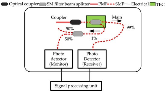
Figure 4.
Same experimental setup as Figure 3, but a TEC was added to the SM filter beam splitter.
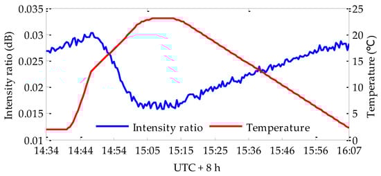
Figure 5.
Intensity ratio results with the same experimental setup shown in Figure 4.
After a thermal control function was added to the SM filter beam splitter, we studied the temperature-dependence of the monitoring photodetector. A TEC was added to the monitoring photodetector, as shown in Figure 6, which changed the temperature from 2 °C to 25 °C. There was a high correlation between the intensity ratio fluctuation and temperature, according to the results in Figure 7. An unacceptable fluctuation of 0.015 dB occurred when the temperature changed by 23 °C. We believe that this was due to the etalon effect in the photodetector module. Following these results, a thermal control function was added to the monitoring photodetector as well to keep the temperature stable. With the above improvements, we measured the fluctuation of the normalized intensity ratio, and the results are shown in Figure 8. The fluctuation was reduced to 0.002 dB with no distinct drift, even if the room temperature changed by 10 °C, and the target precision was realized in the OFLT experiment. The results of the verification experiments show that our lidar system was perfectly calibrated after the thermal control of the SM filter beam splitter and the monitoring photodetector. Kameyama et al. did not report the influence of the temperature-dependent characteristics of the beam splitter on the fluctuation of the normalized intensity ratio, indicating that there are slight differences in the calibration process of systems with different configurations, which is related to the components used in the system.
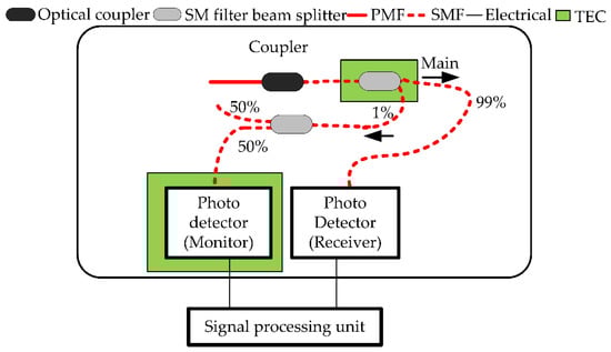
Figure 6.
Same experimental setup as Figure 4, but another TEC was added to the monitoring photodetector.
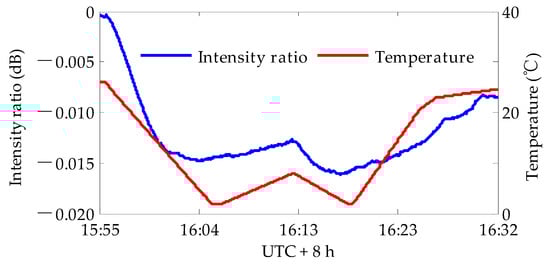
Figure 7.
The results of the intensity ratio with the temperature changes between 2 °C and 25 °C in the monitoring photodetector.
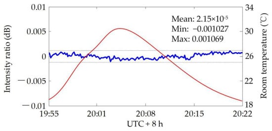
Figure 8.
The results of the normalized intensity ratio after system calibration.
3.4. Improved Speckle Statistics
Based on the speckle principle, the influence of speckle noise on the standard deviation of the normalized intensity ratio was analyzed. We considered the case in which a simultaneous measurement of normalized intensities at the two wavelengths is carried out, and this is repeated times to obtain pairs. We assumed that there is a correlation within the pairs of normalized intensities but no correlation between different pairs. We calculated the ratio of the transmission at the two wavelengths by summing their normalized intensities , respectively, and then taking the ratio. Therefore, the following quantity was evaluated:
We assumed that the two speckle fields were circular complex Gaussian variables and have a degree of correlation described by
The probability density function of u can be expressed as:
where s2 is the degree of correlation between I and I′. From the first and second moments of Equation (8), we obtained the variance of u [11]:
The standard deviation, , is an indication of the uncertainty in the normalized intensity ratio and, hence, determines the accuracy of the measurement taken by the IM-CW IPDA lidar. The standard deviation is plotted in Figure 9 as a function of N for different values of the correlation coefficient. According to the theoretical results, an increase in the correlation coefficient can decrease the standard deviation significantly. The on and off wavelengths in our system can be transmitted simultaneously through the same SM fiber, sharing a common optical power amplifier and transmit-receive apertures. A correlation coefficient greater than 0.9 was very easy to achieve in our system for a suitable scattering surface. In addition, according to Goodman’s speckle theory, a moving diffuser can reduce the correlation time, , which means that shortening the smoothing time to average the time-varying normalized intensity ratio can reduce its fluctuations effectively [21,25]. A moving diffuser is not achievable in actual remote sensing measurements. In this paper, a vibration motor was installed on the telescope, where the centrifugal force generated by the high-speed rotation of a shaft and eccentric block can generate an excitation force to make the transmitting beam vibrate in both horizontal and vertical directions [18]. With an increase in rotational speed, the higher vibration frequency of the beam means that the diffuser moves faster.
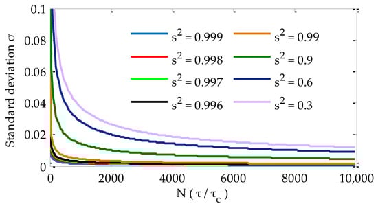
Figure 9.
Standard deviation of the normalized intensity ratio as a function of the smoothing time with different correlation coefficients.
According to the dual frequency speckle cross-correlation theory, the correlation coefficient is also related to the scattering depth and wavelength separation [26]. We assumed that the scattering field was a circular complex Gaussian variable and that the cross-correlation function of the scattering field between two wavelengths separated by is given by
where is the field at wavelength backscattered from a one-dimensional scatter, is the wavelength separation between on and off wavelengths, and is the scattering amplitude at each point and is taken to be a Gaussian profile. The normalized field correlation function is expressed as:
where is the 1/e radius of the intensity. Then, is equal to , by virtue of the Siegert relation. We assumed that the effective target depth was a constant, and so a small results in a high correlation. This reminds us to select the wavelengths with a small wavelength separation between on and off, providing the potential for improving the precision of the IPDA system. As detailed in Section 4, laboratory experiments were designed to verify the theoretical analysis above.
4. Experiments and Results
4.1. Analysis of Speckle Suppression
The improved system based on the research results in Section 3 is shown in Figure 10, where the green box represents the thermal control function and a vibration motor was installed behind the optical antenna. Experiments on a short path (10 cm), where the absorption of CO2 was negligible, were carried out in the laboratory in order to investigate the predictions of the speckle statistical theory under controlled conditions. The lidar output beam illuminated a white painted wall, similar to a Lambertian scatter, and the illumination of many scattering centers resulted in complex Gaussian fluctuation statistics [9]. First, the wavelengths of the on and off seed lasers were adjusted to the and values in Table 1, with a wavelength separation of 16 GHz. The motor was kept stationary, and we calculated the correlation coefficient and standard deviation with different smoothing times. Then, we changed the motor speed and repeated the above steps. The results, as shown in Figure 11, were in accordance with the theoretical analysis. A shorter smoothing time could achieve the target accuracy of the normalized ratio with an increase in the motor speed. The fluctuation of the normalized ratio decreased greatly with the increasing motor speed, as shown in Figure 12. Table 2 shows the correlation coefficient of the normalized intensities between on and off wavelengths, as well the mean and standard deviation of the normalized ratio with different motor speeds. The correlation coefficient increased with the acceleration of the motor speed. However, the mean value of the normalized ratio was different when the motor is rotating and stationary, due to the bias caused by motor rotation.
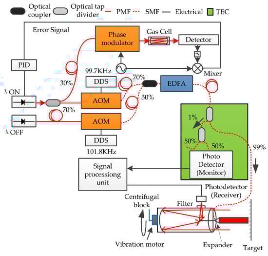
Figure 10.
The improved system configuration. The green box represents the thermal control function, and a vibration motor is installed behind the telescope.
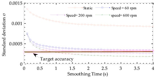
Figure 11.
The standard deviation of the normalized intensity ratio as a function of the smoothing time with different motor speeds.
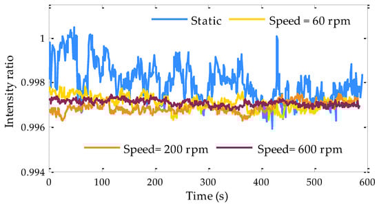
Figure 12.
The normalized intensity ratio with different motor speeds.
Table 2.
Correlation coefficients of the normalized intensities between the on and off wavelengths with different motor speeds.
indicates the average of the normalized ratio, and is the standard deviation of the normalized ratio.
Next, we verified the influence of the wavelength difference between the on and off wavelengths on the correlation coefficient and the fluctuation of the normalized intensity ratio. The motor speed was kept at 600 rpm, the correlation coefficient and normalized intensity ratio were recorded when the on and off wavelengths were adjusted to and (), and and (), respectively. The results are shown in Figure 13. When the wavelength difference between the on and off wavelengths was small, a large correlation coefficient and a smaller fluctuation of the normalized intensity ratio were obtained. These experimental results are consistent with the theoretical analysis. Finally, we chose the motor speed of 600 rpm, and selected and , with smaller wavelength difference, instead of and as the ON and OFF laser wavelengths.
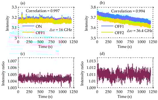
Figure 13.
Intensity time-series for different wavelength separations; (a) intensity of on and off wavelengths separated by 16 GHz; (b) intensity of on and off wavelengths separated by 36.4 GHz; (c) intensity ratio of time-series in (a) after 1 s of smoothing time; (d) intensity ratio of time-series in (b) after 1 s of smoothing time.
4.2. CO2 Concentration Outcomes
Before the field measurement, a zero offset calibration process was first carried out using off-off line testing. Both wavelengths of the improved system were adjusted to the λoff_1 values in Table 1 during the process of the zero offset calibration. In this case, the atmospheric extinction coefficient and target reflectance of the two wavelengths are the same. The effect of speckle noise was very small, as the speckle field between the two wavelengths was highly correlated. With this arrangement, and according to Equation (3), the measured differential optical depth is expected to be zero. An open-path measurement experiment was done in Hongkou District, Shanghai, China, with the dual wavelengths and a concrete exterior wall surface 580 m away as a reflective hard-target. The integral path is shown by an orange double-arrow line in Figure 14. As shown in Figure 15, the correlation coefficient of the normalized intensities of two channels was greater than 0.9997, as the wavelength separation was close to zero. The CO2 concentration results in Figure 16 show that a 5 ppm offset from 0 ppm remained, which could be eliminated by correction. The drift of the concentration baseline was less than 1 ppm. On this path, we adjusted the wavelength of the on laser to the wavelength in Table 1, and an in situ CO2 sensor (Instrumentation for Biological Sciences Ltd., Li-7500A CO2/H2O Analyzer) was placed on the path. After correcting the fixed offset (5 ppm), the measurement results of the CO2 concentration on this path were obtained for 21 h in summer (with a 10 s average measurement interval). The measurement results of the in situ sensor (shown in the rectangular frame in Figure 17) changed drastically due to rain during this period, where the raindrops fell on the window mirror of the open optical path of the Li-7500 to form interference. The measurement of the IPDA lidar was not affected by the rainfall process. In other time periods, the diurnal variations measured by the IPDA lidar were consistent with those of the in situ sensor. The standard deviation of the comparison error between the IPDA lidar and in situ sensor was about 5.566 ppm, as shown in Figure 18. Figure 19 shows the measurement results of the IPDA lidar and the in situ sensor in summer shower weather. The in situ sensor could not work normally for most of the time. There were no obvious peak and valley for the diurnal variations of the CO2 concentration, according to the IPDA lidar measurement results in the shower weather.
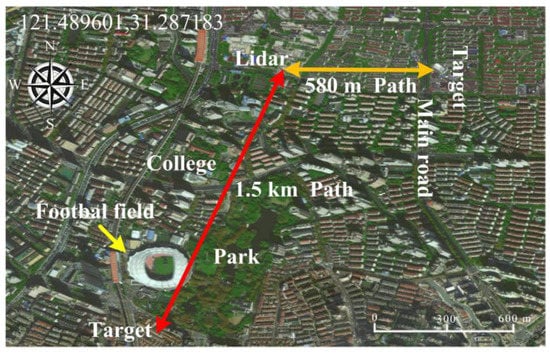
Figure 14.
Integration paths for IPDA lidar testing. The orange double arrow line is the 580 m horizontal path. The red double arrow line is the 1.5 km horizontal path. The base map comes from the China National Platform for Common Geospatial Information Services (http://www.tianditu.gov.cn/).
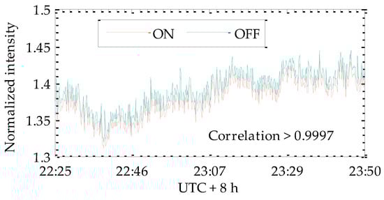
Figure 15.
Normalized intensities with dual off wavelengths.
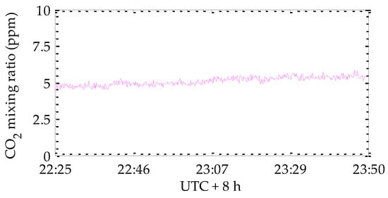
Figure 16.
IPDA lidar CO2 mixing ratio offset measurement using off-off line testing.
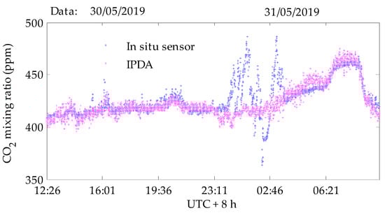
Figure 17.
Simultaneous measurements of the diurnal variations of atmospheric CO2 with the improved IPDA lidar system and an in situ sensor. Black boxes indicate rainy weather. The integral path length is 580 m.
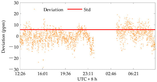
Figure 18.
The discrepancy between the measured CO2 concentration by the IPDA system and in situ sensor on the 580 m horizontal path.
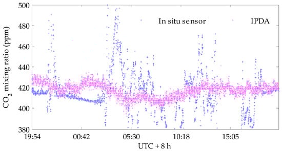
Figure 19.
Simultaneous measurements of the diurnal variations of atmospheric CO2 with the improved IPDA lidar system and an in situ sensor. The integral path length is 580 m and the weather was rainy.
Figure 20 shows the diurnal variation of the horizontal column-averaged CO2 concentrations obtained by the improved system on 7 November 2019 over a 1.5 km path (red double arrow line in Figure 14). The diurnal variations measured by the IPDA lidar were consistent with the in situ sensor. The standard deviation of the comparison error between the IPDA lidar and the in situ sensor was about 5.987 ppm, as shown in Figure 21. Figure 22 shows the measurement results of the IPDA lidar on this path for five consecutive days (18–22 October 2019) in autumn. The weather was clear throughout the measurement time. The characteristics of the diurnal variations of CO2 concentrations in five days are similar and obvious, showing a clear change rule of one peak and one valley. During the day, the CO2 concentration reaches its lowest value around 14 o’clock, which is close to the atmospheric background concentration. This might be because the atmospheric convection and horizontal activities are more active during this period, which is conducive to the diffusion of pollutants. In addition, during this period, plants have strong photosynthetic activity and absorb a greater amount of CO2. After 15 o’clock, the CO2 generated by soil, biological respiration and industrial production accumulated in the near-surface atmosphere and the CO2 concentration began to rise slowly, reaching its highest value before sunrise. After sunrise, the CO2 concentration can be seen to drop rapidly.
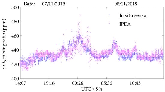
Figure 20.
Simultaneous measurements of the diurnal variations of atmospheric CO2 with the improved IPDA system and an in situ sensor. The integral path length is 1.5 km and the weather was sunny.
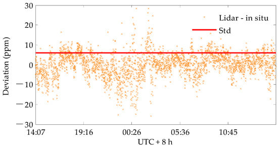
Figure 21.
The discrepancy between the measured CO2 concentration by the IPDA system and in situ sensor on the 1.5 km horizontal path.
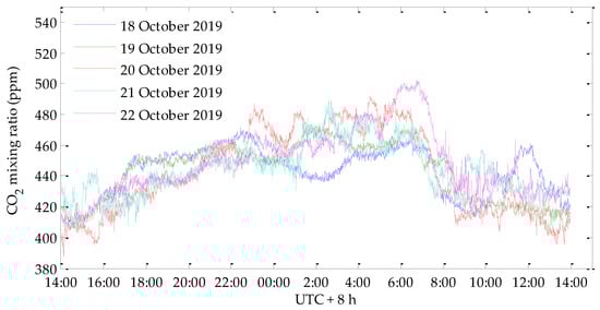
Figure 22.
The measurement results of the IPDA lidar over five consecutive days in autumn (18–22 October 2019).
5. Conclusions
A 1.57 μm IM-CW IPDA fiber-based lidar capable of remotely sensing atmospheric CO2 was demonstrated. The system utilizes advanced EDFA technology to achieve the simultaneous transmission of on and off lasers through the same single-mode fiber-based optical system, sharing common transmit-receive apertures. The on and off lasers are intensity modulated with CW signals at slightly different frequencies (e.g., 99.7 kHz and 101.8 kHz), in order to distinguish the received on and off radiation. In the first trial, the detected CO2 mixing ratio strongly fluctuated around the expected 410 ppm ambient concentration, with minimum and maximum values of 300 and 600 ppm, respectively. Therefore, it was believed that unknown sources of systematic errors caused large fluctuations in the CO2 concentration, indicating the necessity for system calibration. The temperature sensitivity of some optical components and the speckle effect caused by the random scattering of targets and atmospheric turbulence were determined to be the main reasons for the large fluctuations in the DAOD measurements through the accumulation of results from preliminary experiments. Following the results of the OFLT experiment, a thermal control function was added to the SM filter beam splitter and the monitoring photodetector, after which the fluctuation of the normalized intensity ratio was less than 0.003 dB, corresponding to a CO2 concentration precision of 1 ppm for a 1 km path. In the preliminary experiments, the CNRs were very high, but the random error of the CO2 concentration measurement value was quite large, which means that increasing the transmitting optical power does not contribute much to improve the performance. This is because the speckle-related SNR limits short-term fluctuations. We added a vibration motor at the end of the optical antenna to reduce the speckle correlation time, which has not yet been reported in the literature, to the best of our knowledge. The experimental results demonstrated that the fluctuation of the normalized intensity ratio was much smaller when the motor vibrated than when the motor was stationary. The faster the motor vibrated, the smaller the fluctuation of the normalized intensity ratio. We have demonstrated, using theoretical and modeling techniques, that highly correlated speckle has a great advantage in reducing the variance of the DAOD. The degree of correlation is determined by the wavelength separation between the on and off lasers. Therefore, a smaller wavelength separation has the potential for improving the accuracy of IPDA lidar systems. In a laboratory situation without atmospheric absorption and interference, the reflective target was approximately a Lambertian scatter, and the fluctuation of the normalized intensity ratio with the on and off frequencies separated by 36.4 GHz was twice as large as that when the wavelength separation was 16 GHz. The results of the laboratory experiments were consistent with the theoretical predictions. We also analyzed the CO2 concentration measurement performance of this system after implementing the improvements described above. The diurnal variations measured by the IPDA lidar were consistent with an in situ sensor.
Unfortunately, we cannot discuss the speckle decorrelation caused by atmospheric turbulence any further, as we had no chance to measure the turbulence conditions.
Author Contributions
Conceptualization, G.H.; methodology, H.L., W.K. and T.C.; software, X.L.; validation, X.L.; formal analysis, X.L.; investigation, X.L.; resources, G.H.; data curation, X.L.; writing—original draft preparation, X.L.; writing—review and editing, T.C.; visualization, X.L.; supervision, G.H.; project administration, G.H.; funding acquisition, G.H. All authors have read and agreed to the published version of the manuscript.
Funding
This research was funded by National Key R&D Program of China (grant number 2017YFB0504000), the National Natural Science Foundation of China (grant numbers 61875219, 61805268), and the Key Laboratory Foundation of Chinese Academy of Sciences (grant number CXJJ-19S019).
Conflicts of Interest
The authors declare no conflict of interest.
References
- Houweling, S.; Aben, I.; Breon, F.M.; Chevallier, F.; Deutscher, N.; Engelen, R.; Gerbig, C.; Griffith, D.; Hungershoefer, K.; Macatangay, R.; et al. The importance of transport model uncertainties for the estimation of CO2 sources and sinks using satellite measurements. Atmos. Chem. Phys. 2010, 10, 9981–9992. [Google Scholar] [CrossRef]
- Plattner; GianKasper. IPCC, 2014: Climate Change 2014: Synthesis Report. Contribution of Working Groups I, II and III to the Fifth Assessment Report of the Intergovernmental Panel on Climate Change. J. Roman. Stud. 2014, 4, 85–88. [Google Scholar]
- Miller, C.; Crisp, D.; DeCola, P.; Olsen, S.; Randerson, J.; Michalak, A.; Alkhaled, A.; Rayner, P.; Jacob, D.; Suntharalingam, P.; et al. Precision requirements for space-based XCO2 data. J. Geophys. Res. 2007, 112. [Google Scholar] [CrossRef]
- Refaat, T.; Ismail, S.; Koch, G.; Rubio, M.; Mack, T.; Notari, A.; Collins, J.; Lewis, J.; Young, R.; Choi, Y.; et al. Backscatter 2-μm Lidar Validation for Atmospheric CO2 Differential Absorption Lidar Applications. IEEE Trans. Geosci. Remote Sens. 2011, 49, 572–580. [Google Scholar] [CrossRef]
- Gibert, F.; Flamant, P.H.; Bruneau, D.; Loth, C. Two-micrometer heterodyne differential absorption lidar measurements of the atmospheric CO2 mixing ratio in the boundary layer. Appl. Opt. 2006, 45, 4448–4458. [Google Scholar] [CrossRef]
- Gibert, F.; Pellegrino, J.; Edouart, D.; Cénac, C.; Lombard, L.; Le Gouët, J.; Nuns, T.; Cosentino, A.; Spano, P.; Di Nepi, G. 2-μm double-pulse single-frequency Tm:fiber laser pumped Ho:YLF laser for a space-borne CO2 lidar. Appl. Opt. 2018, 57, 10370–10379. [Google Scholar] [CrossRef]
- Gibert, F.; Edouart, D.; Cénac, C.; Le Mounier, F.; Dumas, A. 2-μm Ho emitter-based coherent DIAL for CO2 profiling in the atmosphere. Opt. Lett. 2015, 40, 3093–3096. [Google Scholar] [CrossRef]
- Kameyama, S.; Imaki, M.; Hirano, Y.; Ueno, S.; Kawakami, S.; Sakaizawa, D.; Kimura, T.; Nakajima, M. Feasibility study on 1.6 μm continuous-wave modulation laser absorption spectrometer system for measurement of global CO2 concentration from a satellite. Appl. Opt. 2011, 50, 2055–2068. [Google Scholar] [CrossRef]
- Amediek, A.; Fix, A.; Wirth, M.; Ehret, G. Development of an OPO system at 1.57 μm for integrated path DIAL measurement of atmospheric carbon dioxide. Appl. Phys. B 2008, 92, 295–302. [Google Scholar] [CrossRef]
- Abshire, J.B.; Ramanathan, A.; Riris, H.; Mao, J.P.; Allan, G.R.; Hasselbrack, W.E.; Weaver, C.J.; Browell, E.V. Airborne Measurements of CO2 Column Concentration and Range Using a Pulsed Direct- Detection IPDA Lidar. Remote Sens. 2014, 6, 443–469. [Google Scholar] [CrossRef]
- Ridley, K.D.; Pearson, G.N.; Harris, M. Improved speckle statistics in coherent differential absorption lidar with in-fiber wavelength multiplexing. Appl. Opt. 2001, 40, 2017–2023. [Google Scholar] [CrossRef] [PubMed]
- Dobler, J.T.; Harrison, F.W.; Browell, E.V.; Lin, B.; McGregor, D.; Kooi, S.; Choi, Y.; Ismail, S. Atmospheric CO2 column measurements with an airborne intensity-modulated continuous wave 1.57 μm fiber laser lidar. Appl. Opt. 2013, 52, 2874–2892. [Google Scholar] [CrossRef] [PubMed]
- Lin, B.; Nehrir, A.R.; Harrison, F.W.; Browell, E.V.; Ismail, S.; Obland, M.D.; Campbell, J.; Dobler, J.; Meadows, B.; Fan, T.F.; et al. Atmospheric CO2 column measurements in cloudy conditions using intensity-modulated continuous-wave lidar at 1.57 micron. Opt. Express 2015, 23, A582–A593. [Google Scholar] [CrossRef] [PubMed]
- Browell, E.V.; Dobler, J.; Kooi, S.A.; Choi, Y.; Harrison, F.W.; Moore, B., III; Zaccheo, T.S. Airborne Validation of Laser Remote Measurements of Atmospheric Carbon Dioxide. In Proceedings of the ILRC25 (25th International Laser Radar Conference), St. Petersburg, Russia, 5–9 July 2010; pp. 779–782. [Google Scholar]
- Browell, E.; Dobler, J.; Kooi, S.; Fenn, M.; Choi, Y.; Vay, S.; Harrison, F.; Moore, B. Airborne laser CO2 column measurements: Evaluation of precision and accuracy under a wide range of surface and atmospheric conditions. In Proceedings of the American Geophysical Union Fall Meeting 2011, San Francisco, CA, USA, 5–9 December 2011. [Google Scholar]
- Browell, E.V.; Dobbs, M.E.; Dobler, J.; Kooi, S.; Moore, B. Airborne demonstration of 1.57-micron laser absorption spectrometer for atmospheric CO2 measurements. In Proceedings of the 24th International Laser Radar Conference, Boulder, CO, USA, 23–27 June 2008. [Google Scholar]
- Kameyama, S.; Imaki, M.; Hirano, Y.; Ueno, S.; Kawakami, S.; Sakaizawa, D.; Nakajima, M. Development of 1.6 μm continuous-wave modulation hard-target differential absorption lidar system for CO2 sensing. Opt. Lett. 2009, 34, 1513–1515. [Google Scholar] [CrossRef]
- Kameyama, S.; Imaki, M.; Hirano, Y.; Ueno, S.; Kawakami, S.; Sakaizawa, D.; Nakajima, M. Performance improvement and analysis of a 1.6 μm continuous-wave modulation laser absorption spectrometer system for CO2 sensing. Appl. Opt. 2011, 50, 1560–1569. [Google Scholar] [CrossRef]
- Gordon, I.E.; Rothman, L.S.; Hill, C.; Kochanov, R.V.; Tan, Y.; Bernath, P.F.; Birk, M.; Boudon, V.; Campargue, A.; Chance, K.V.; et al. The HITRAN2016 molecular spectroscopic database. J. Quant. Spectrosc. Radiat. Transf. 2017, 203, 3–69. [Google Scholar] [CrossRef]
- Liu, H.; Chen, T.; Shu, R.; Hong, G.; Zheng, L.; Ge, Y.; Hu, Y. Wavelength-locking-free 1.57 µm differential absorption lidar for CO2 sensing. Opt. Express 2014, 22, 27675–27680. [Google Scholar] [CrossRef]
- Cassé; Gibert; Edouart; Chomette; Crevoisier. Optical Energy Variability Induced by Speckle: The Cases of MERLIN and CHARM-F IPDA Lidar. Atmosphere 2019, 10, 540. [Google Scholar] [CrossRef]
- Refaat, T.F.; Singh, U.N.; Yu, J.; Petros, M.; Remus, R.; Ismail, S. Double-pulse 2-μm integrated path differential absorption lidar airborne validation for atmospheric carbon dioxide measurement. Appl. Opt. 2016, 55, 4232–4246. [Google Scholar] [CrossRef]
- Du, J.; Zhu, Y.; Li, S.; Zhang, J.; Sun, Y.; Zang, H.; Liu, D.; Ma, X.; Bi, D.; Liu, J.; et al. Double-pulse 1.57 μm integrated path differential absorption lidar ground validation for atmospheric carbon dioxide measurement. Appl. Opt. 2017, 56, 7053–7058. [Google Scholar] [CrossRef] [PubMed]
- Sakaizawa, D.; Kawakami, S.; Nakajima, M.; Tanaka, T.; Morino, I.; Uchino, O. An airborne amplitude-modulated 1.57 μm differential laser absorption spectrometer: Simultaneous measurement of partial column-averaged dry air mixing ratio of CO2 and target range. Atmos. Meas. Tech. 2013, 6, 387–396. [Google Scholar] [CrossRef]
- Freund, I.; Joseph, W. Goodman: Speckle Phenomena in Optics: Theory and Applications. J. Stat. Phys. 2008, 130, 413–414. [Google Scholar] [CrossRef]
- Zhang, G.; Wu, Z. Two-frequency mutual coherence function of scattering from arbitrarily shaped rough objects. Opt. Express 2011, 19, 7007–7019. [Google Scholar] [CrossRef]
© 2020 by the authors. Licensee MDPI, Basel, Switzerland. This article is an open access article distributed under the terms and conditions of the Creative Commons Attribution (CC BY) license (http://creativecommons.org/licenses/by/4.0/).