Article

Influence of Novaya Zemlya Bora on Sea Waves: Satellite Measurements and Numerical Modeling

by
Anna A. Shestakova
1,*,
Stanislav A. Myslenkov
2,3,4 and
Alexandra M. Kuznetsova
5
1
A.M. Obukhov Institute of Atmospheric Physics of the Russian Academy of Science, 119017 Moscow, Russia
2
Faculty of Geography, Lomonosov Moscow State University, 119991 Moscow, Russia
3
Shirshov Institute of Oceanology of the Russian Academy of Science, 117997 Moscow, Russia
4
Hydrometeorological Research Centre of the Russian Federation, 123242 Moscow, Russia
5
Institute of Applied Physics of the Russian Academy of Science, 603950 Nizhny Novgorod, Russia
*
Author to whom correspondence should be addressed.
Atmosphere 2020, 11(7), 726; https://doi.org/10.3390/atmos11070726
Submission received: 21 May 2020 / Revised: 1 July 2020 / Accepted: 2 July 2020 / Published: 7 July 2020
(This article belongs to the Special Issue Atmospheric Processes Shaping Polar Climate)

Abstract

:
This paper investigates for the first time sea waves during Novaya Zemlya bora—a downslope windstorm on the western coast of the archipelago during eastern winds—using a statistical and case-study approach. Statistical analysis of altimeter data off the western coast of Novaya Zemlya during bora shows that, despite strong wind forcing, the frequency of hazard wave heights was low due to the limited fetch. This result was confirmed by the high-resolution numerical simulations of two severe bora episodes. However, the influence of bora on sea waves in some cases was significant: bora increased wave height at a distance from shore greater than 200 km and wave height anomaly was up to 2–3 m. The influence of the wind input parametrization choice during bora is great in the coastal region; however, parametrizations with fetch-limited modifications and strong-wind adopted aerodynamic drag coefficient do not improve the modeling results in the open sea where altimeter data are available.

1. Introduction

Novaya Zemlya bora is a strong gusty wind (downslope windstorm) occurring on the western and eastern coasts of Novaya Zemlya during air flow over the mountain ridge. Severity of this wind has been known from the first half of the 20th century [1]. Frequency of wind speed higher than 30 m s−1 during bora on the western coast is 4%, and the wind attains a maximal speed of 48 m s−1 [2].
Downslope windstorms in the Arctic cause hazardous weather events such as ship icing [3], poor visibility [4], and rapid ice drift [5]. Local coastal winds can also lead to a significant local increase in the height of the wind waves [6]. For instance, wave height near the coast in the Novorossiysk region increases in simulations that take into account the Novorossiysk bora when compared with simulations without the bora [7].
An increase in wave height should also be expected during downslope windstorms in the Arctic. This is especially likely on the western coast of Novaya Zemlya where wind speed reaches its greatest value in the entire Arctic and where most of the year the coast is ice-free, which distinguishes the Novaya Zemlya bora from downslope windstorms in Tiksi Bay, Pevek, and on Wrangel Island [8]. Despite the large number of studies on the Novaya Zemlya bora [2,8,9,10,11,12,13,14], hazardous weather events associated with bora including storm waves have never been investigated.
Storm waves affect the efficiency and safety of maritime operations, leading to significant economic cost and even fatalities. Extreme natural phenomena in the coastal zone are usually strongly localized in space and time, and because of their low frequency, do not readily lend themselves to statistical estimation. This is why understanding the mechanism of these phenomena, assessing, and minimizing the risks associated with them is one of the most urgent tasks of operational oceanography.
Sea waves caused by winds such as bora winds can hardly be described using classical methods adopted in describing fetch-limited waves caused by stationary offshore winds more uniform in space [15,16]. Downslope windstorms themselves are known not to extend very far from the lee slopes [8,17,18]. Due to the so-called hydraulic jump (see, for example, [19]), the flow returns from the supercritical state (shallow and fast flow) to the subcritical state (deep and slow flow), which is expressed in a sharp alternation of strong-wind (near the foot of the mountain ridge) and weak-wind (downstream, in the open sea) zones (so-called wakes). Gap winds that always accompany bora have a different structure and occur downstream from straits, river valleys, and passes and spread over 100–200 km in the sea [20], but are usually weaker than downslope windstorms. It is a complex spatial structure of wind field during bora and gap winds, which would lead to deviations from the classical pattern of wave propagation during offshore winds. For instance, Shimada and Kawamura [21] showed significant difference in the frequency-direction wave spectra between wakes and neighboring gap wind jets.
The paper focused on sea waves during the Novaya Zemlya bora on the west coast of the archipelago and had three tasks. Its first task, most relevant in practical terms, was to evaluate the frequency of extreme waves (creating risks in navigation) during bora. To this end, a statistical analysis of satellite altimetry observations was carried out. The second task was to estimate the contribution of the Novaya Zemlya bora to sea wave formation, in order to see whether it could be neglected, or whether the waves caused by bora (hereafter, “bora-caused waves”) must be taken into account. To address this problem, altimetry observations and high-resolution simulations, which explicitly resolve bora, were compared with a much rougher wave reanalysis, in which the bora effect is not resolved or it is weak. Finally, the third task was to evaluate the features of the bora-caused waves including the wave steepness, wave spectral characteristics, spatial features of the wave field, and the distance from the coast at which the highest and steepest waves were observed. In addition, we performed numerical experiments with different wind input parametrizations and modified nonlinear wave interaction scheme in the wave model. These experiments allowed us to evaluate the effect of short fetches characteristic of orographic winds on the wave modeling results under bora conditions.

2. Data and Methods

2.1. Bora Calendar

To determine the bora periods, we used the observational data at the Malye Karmakuly weather station located on the western coast of the South Island of the Novaya Zemlya archipelago (see Figure 1). Data arse freely available on the website of the Research Institute of Hydrometeorological Information–World Data Center [22]. The calendar of bora episodes was created for the period of 1976–2016 according to the method described in [2]. However, unlike in [2], we used more rigorous criterion of the mean 10-min wind speed exceeding 15 m s−1 and wind direction in the interval 70–120°. This meant to exclude cases of weak bora that could not have any significant effect on sea waves. A total of 9124 times or 2483 days with bora were selected.

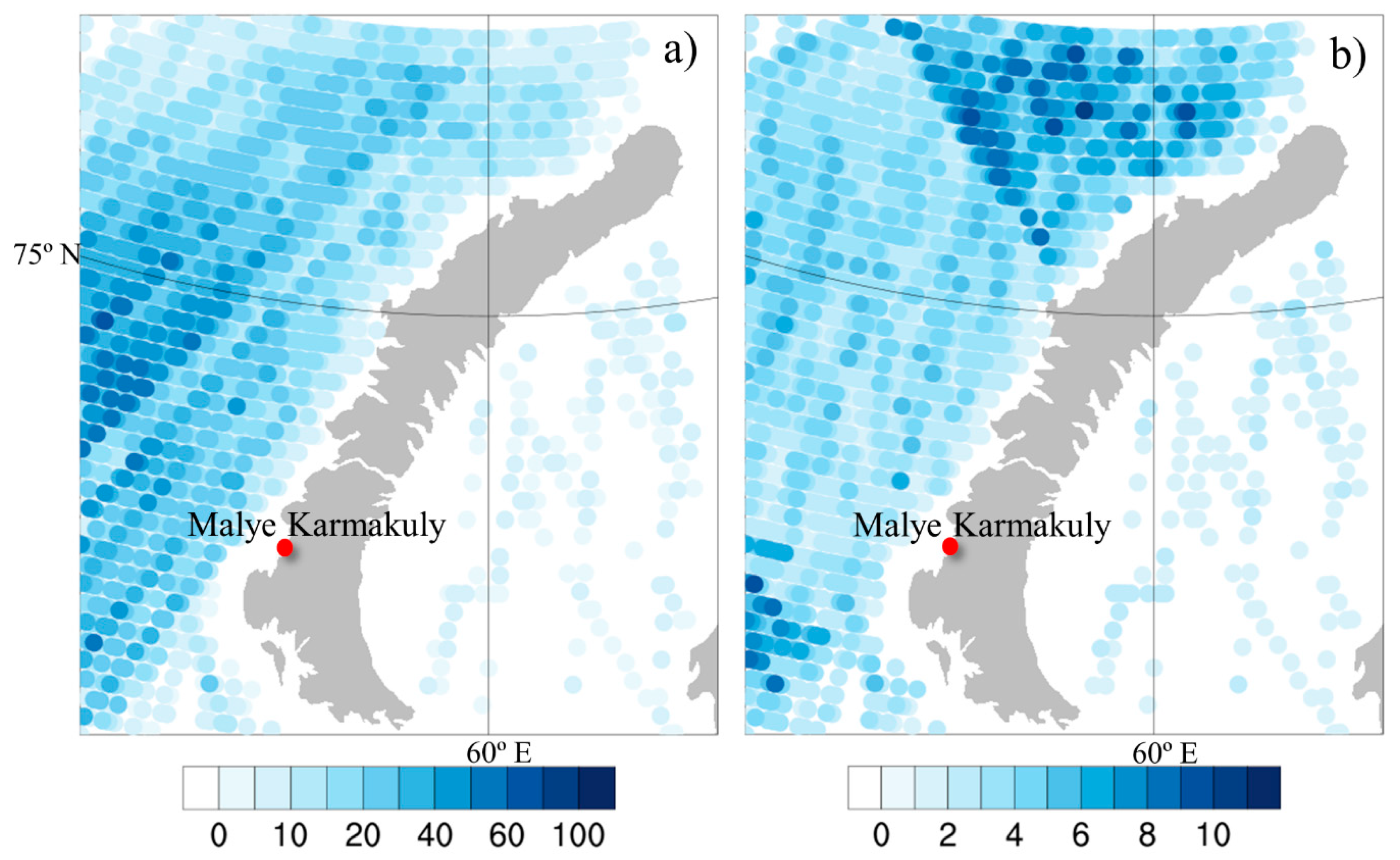
2.2. Satellite Altimetry

There are no systematic in situ observations of sea waves during bora in the study area, therefore, we used satellite altimeter measurements as the main source of information in this study as well as in several other studies dealing with the sea waves in the Arctic (e.g., [16,23]). We created a database of altimetry measurements of wind speed and significant wave height (SWH) in the Novaya Zemlya region (46° E–66° E longitude, 70° N–78° N latitude) during bora from CryoSat, Envisat, ERS (European Remote-Sensing Satellite), Geosat, GFO (GEOSat Follow-on), SARAL (Satellite with ARGOS and AltiKa), and Sentinel satellites for the period from 1985 to 1988 and from 1991 to 2018. This regional database of altimetry measurements is based on the calibrated altimeter observations provided by Ribal and Young [24] and distributed by IMOS (Integrated Marine Observing System) through the Australian Ocean Data Network portal [25]. Measured wave height and backscatter coefficients in the Ku-band (frequency range 12–18 GHz), C-band (frequency range 4–8 GHz), and Ka-band for SARAL (frequency range 35.75 GHz +/− 250 MHz) averaged over a one second sampling interval (which approximately corresponds to 6–7 km in space) were used. The root mean square error (RMSE) of SWH from different altimeters verified against observational data is usually estimated at about 0.3 m [26]. The quality of the AltiKa altimeter data from the SARAL satellite is better, where the RMSE of SWH is 0.21 m [27].
In total, our altimetry database included 28,309 measurements, 575 times or 507 days with bora. The following data were excluded from the database:
-
values with standard deviation of the altimeter SWH exceeding 0.4;
-
values with SWH lower than 0.3 m;
-
values with distance to the shore closer than 15 km; and
-
values with distance to the nonzero ice concentration closer than 10 km.
Wind speed derived from satellite altimeters is calculated from the normalized radar cross section using standard algorithms [28]. Altimeter wind in coastal areas should be treated with caution [29,30], since standard wind calculation schemes are tuned to the ocean and developed waves. On average, the accuracy of altimeter wind speed compared with buoy measurements is 1.5 m s−1 [31]. For Altika, the RMSE of wind speed is 1.75 m s−1, with a bias of 0.25 m s−1 [27].
To evaluate the statistical characteristics, altimeter SWH and wind speed were interpolated onto the grid with a spacing of 20 km. Spatial-temporal average and maximum value were calculated inside each grid cell. The largest number of observations was in the southwestern part of the study area. Near the coast of Novaya Zemlya and in the north, the number of observations was much smaller, from 5 to 50 in each cell (Figure 1a). At the same time, the number of days when satellite observations were available during bora was from 2 to 12 with a maximum in the north of the region (Figure 1b).

2.3. Wave Reanalysis

Wave reanalysis in the Barents Sea and North Atlantic was created on the basis of calculations of the Wave Watch III (WW3) wave model version 4.18 for the period 1979–2016 [32]. The calculations were performed using an unstructured grid. This grid consists of 16,792 nodes; the spatial resolution varies from ~15 km for the Barents Sea to ~50 km for the northern part of the Atlantic Ocean. The model output includes SWH, wave direction, mean period and wavelength; temporal resolution of the model output is 3 h. Wind forcing for wave modeling was obtained from the Climate Forecast System Reanalysis (CFSR) (1979–2010) with a spatial resolution of ~0.3° [33] and the Climate Forecast System version 2 reanalysis (2011–2017) with a spatial resolution of ~0.2° [34].
Wave climate and storm activity in the Barents Sea was previously investigated using this wave reanalysis [32,35,36]. However, the spatial resolution of the wave model and atmospheric forcing was not sufficient to adequately reproduce orographic winds [9,37]. Figure 2 clearly demonstrates this: SWH composite during bora (Figure 2a), calculated from wave reanalysis, differed slightly from the climatic field [32]; the anomaly of wave height near the west coast of Novaya Zemlya was near zero (Figure 2b). Therefore, wave reanalysis here was considered as a background (large-scale) state of the wave field.
When creating the wave reanalysis, the following set of WW3 parameterizations was used: the ST1 scheme for the wave generation; the DIA (Discrete Interaction Approximation) parameterization for nonlinear wave interactions; JONSWAP scheme for bottom friction; and IC0 scheme for sea ice (with ice concentration more than 25%, the grid node is considered to be covered with ice, and the exponential attenuation of wave energy corrected for ice concentration in this node is turned on [38]). The spectral resolution of the model was 36 directions; the frequency range included 36 intervals (from 0.03 to 0.843 Hz). Integration time step for the full equation was 30 min, the time step for the functions of the sources and sinks of wave energy was 30 s; the time step for transmitting energy over the spectrum was 900 s.

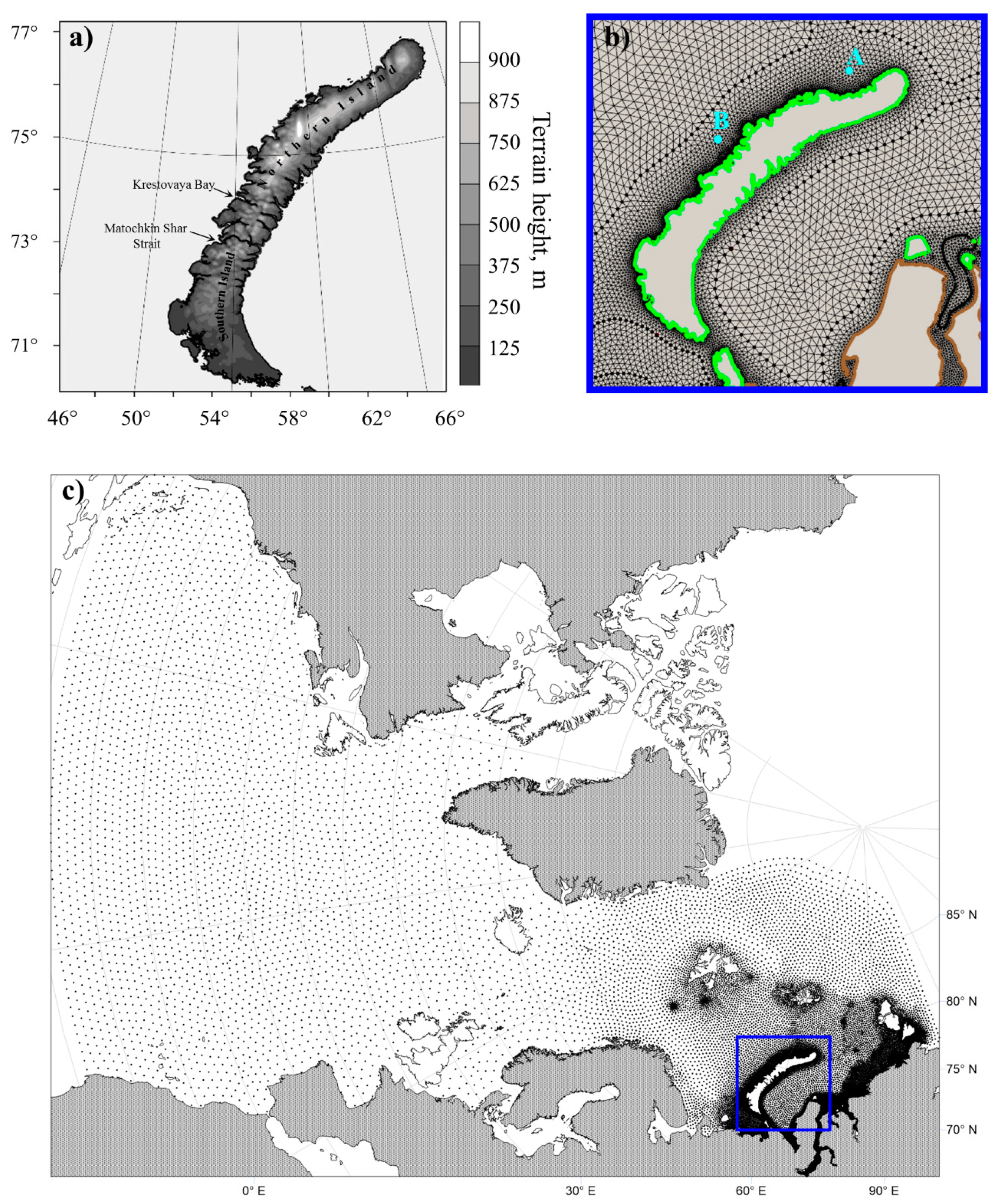
2.4. High-Resolution Wave Modeling

2.4.1. Model Configuration

The sample length of satellite observations in the Novaya Zemlya region is rather small (Figure 1), and the accuracy of altimeter data decreases near the coast [39]. To study sea waves during bora in coastal areas in more detail, we additionally performed numerical wave simulation using the WW3 model with atmospheric forcing from the WRF-ARW (Weather Research and Forecasting—Advanced Research WRF) model for two cases of strong Novaya Zemlya bora on 7–15 January 2006 (hereafter, the “2006 episode”) and 9–12 February 2009 (hereafter, the “2009 episode”). In these episodes, bora occurred both in Malye Karmakuli and in the northern part of the archipelago, reaching a hurricane force (36 m s−1 in the 2006 episode and 40 m s−1 in the 2009 episode). A comparatively large number of satellite observations inside the WRF modeling domain (Figure 3a) were collected during these episodes (246 observations in 2006 and 212 in 2009).
Sea waves were simulated using the WW3 model on an unstructured grid including the Barents and Kara Seas (Figure 3b) as well as the entire northern part of the Atlantic Ocean to take into account the incoming swell (Figure 3c). The spatial resolution in the coastal area around Novaya Zemlya (Figure 3b) was about 1 km. The set of parameterizations coincides with that used to create the wave reanalysis (Section 2.3).
A combination of wind from the Climate Forecast System Reanalysis (CFSR reanalysis) (in the Barents Sea excluding the WRF-ARW domain region, shown in Figure 3a) and the WRF-ARW simulation (in the Novaya Zemlya region) was used as atmospheric forcing for the wave model. Wind speed from the reanalysis and the model was interpolated to the unstructured grid of the wave model. Interpolation was performed using the four nearest nodes (around the node of the wave model grid) of the WRF model grid inside WRF model domain (Figure 3a), or using the four nearest nodes of CFSR reanalysis grid outside the WRF model domain.
Polar WRF-ARW model version 3.4.1 was used to simulate the Novaya Zemlya bora. The WRF-ARW modeling area (Figure 3a) included 249 points in longitude, 269 points in latitude, and 50 vertical levels. The spatial resolution was 3 km; vertical grid spacing monotonically increased with height. The atmospheric model was initialized using the Arctic System Reanalysis version 2 (ASR v.2) [40] with a spatial resolution of 15 km and a temporal resolution of three hours. The model was nudged toward wind, temperature, and humidity observations at the Malye Karmakuly station. Observational nudging is a type of four-dimensional data assimilation and is based on the addition of innovations obtained from the observed values to the model tendency equation. Observational nudging was performed throughout the whole model simulation; the time window for every observation was set at 3 h. The radius of influence of observations was set to 30 km (i.e., 10 model nodes) from the observation point. Nudging coefficients for all variables were set at the default value of 6 × 10⁻⁴. Sea surface temperature was updated every six hours from ASR v.2. The following set of parameterizations was used: the Yonsei University scheme for the boundary layer, the Noah model for the land surface, the RRTMG scheme for radiation fluxes, and the Thompson scheme for cloud microphysics.
The following parameters were analyzed using the simulation data: wind speed and direction at 10 m above ground level (AGL); significant wave height; frequency-direction wave power spectra at points A and B (40 km from the coast) (Figure 3b) as well as the wave steepness. The latter was calculated using the formula introduced by Buckley [41] and used by the National Data Buoy Center [42]:
S = H s / exp 3.3   ln f p ,
where f p is the peak frequency, and H s is the significant wave height. Waves are considered steep when S > 0.002 and very steep when S > 0.004.
To verify the simulation results, model values of wind speed and wave height were compared with altimetry observations closest to the model grid nodes. In this case, only those observations were used that were taken at points closer than 15 km to the grid node. As shown in [43], such a collocation window between satellite altimeters and other data gives the most accurate results. The wind speed observations at Malye Karmakuly station were compared with the modeled wind speed at the grid node closest to the station.

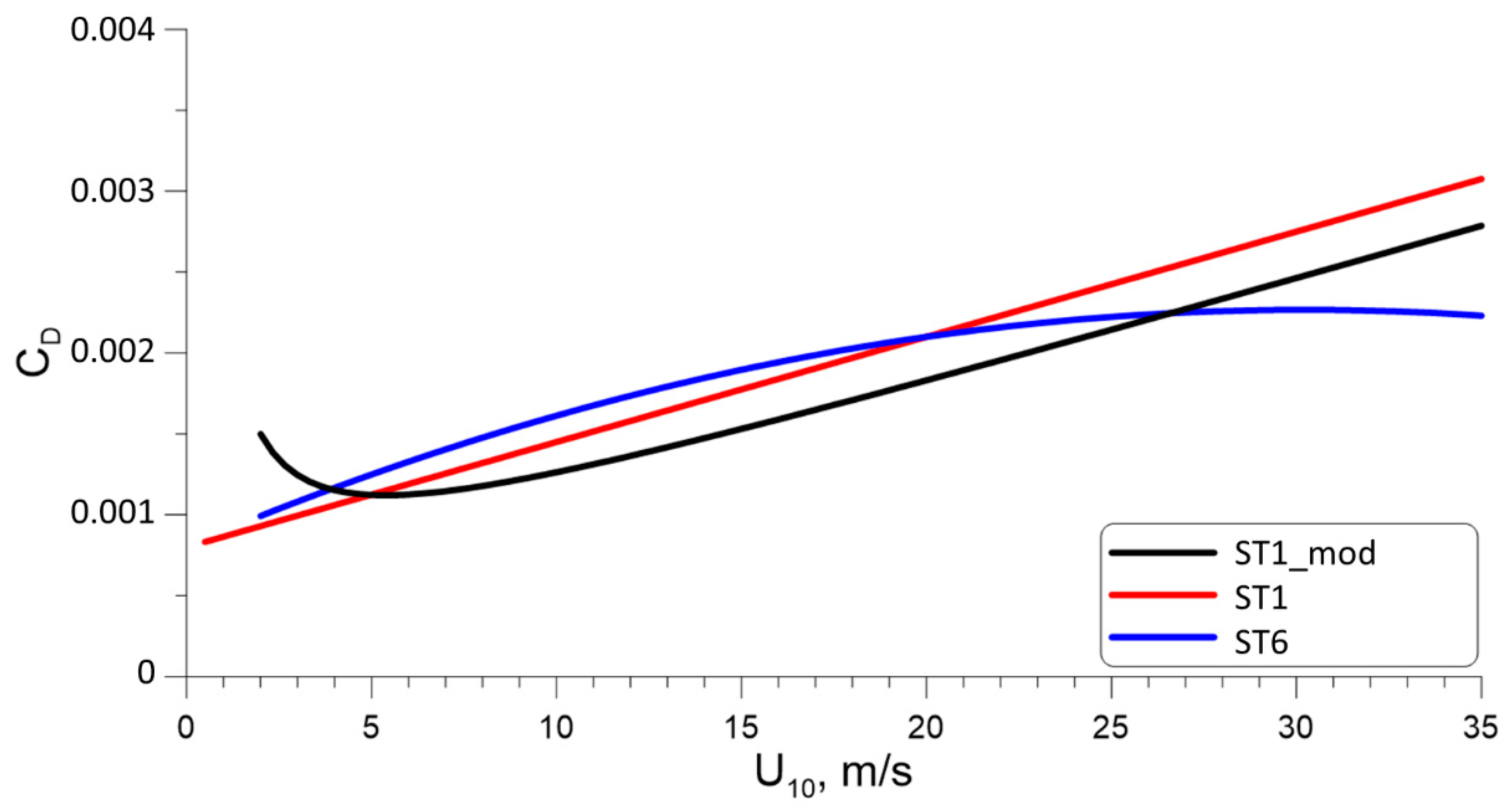
2.4.2. Experiments with Different Wind Input Parameterizations

Three series of simulations were performed to study the effect of wind input parametrizations on the results of sea wave simulation during bora. All other parameterizations in these experiments were set to be identical (see Section 2.4.1).
In the first control experiment (hereafter-ST1), the WAM3 wind input parameterization was used with all the “default” parameters. The dependence of the aerodynamic drag coefficient C D on wind speed at 10 m AGL U 10 can be calculated as follows [44]:
C D U 10 = 0.001 0.8 + 0.65 U 10
However, in the coastal zone and during stormy winds, the dependence of the drag coefficient on wind speed differs from the standard one [45]. Fetch-limited waves are characterized by more intense wind pumping and stronger non-linearity than is the case in the standard parameterization ST1, which is configured for modeling in the open sea. Therefore, in the second experiment (hereafter-ST1_mod) using the same wind input parameterization, the aerodynamic drag coefficient was changed in accordance with the dependence obtained from field data at Gorky Reservoir [46]:
C D U 10 = 0.0019 U 10 1 + 0.0004 + 0.000067 U 10
Comparison with the measurements at Gorky Reservoir showed that the energy transfer over the wave spectrum in the model was too slow, resulting in a less steep waves than those observed [47]. It is the nonlinear four-wave interactions parametrization DIA that determines the rate of the energy transfer over the wave spectrum. Therefore, some parameters in this parametrization were also changed in the ST1_mod experiment. Parameter λ, which determines the difference in the frequencies of interacting harmonics, was set at 0.29 (instead of the “default” 0.25), while parameter C, which determines the contribution of nonlinear four wave interactions to the total spectrum, was set at 3.8 × 10⁷ (instead of 2.78 × 10⁷) [48]. Simulations with the modified coefficients most closely reproduce the observed sea waves at Gorky Reservoir.
In the third experiment (hereafter, ST6), the modern parameterization of wind input ST6 was used [49,50], which was also tested in storm conditions of the North Sea [51]. The parameterization of the drag coefficient in this model has the curvature necessary for hurricane wind simulation:
C D U 10 = 10 4 8.058 + 0.967 U 10 0.016 U 10 2
The corresponding parameters of the nonlinear interactions scheme DIA in ST6 parametrization were: λ = 0.25 and C = 3 × 10⁷. Accounting for the short fetches in the ST6 parametrization is absent in the current version of the WW3 model, however, it can be expected in the future versions of the model [52].
A comparison of the aerodynamic drag parameterizations in the wind input parametrizations used is shown in Figure 4. It can be expected that the use of different parameterizations of C D U 10 will considerably affect the wave growth rate.

3. Results

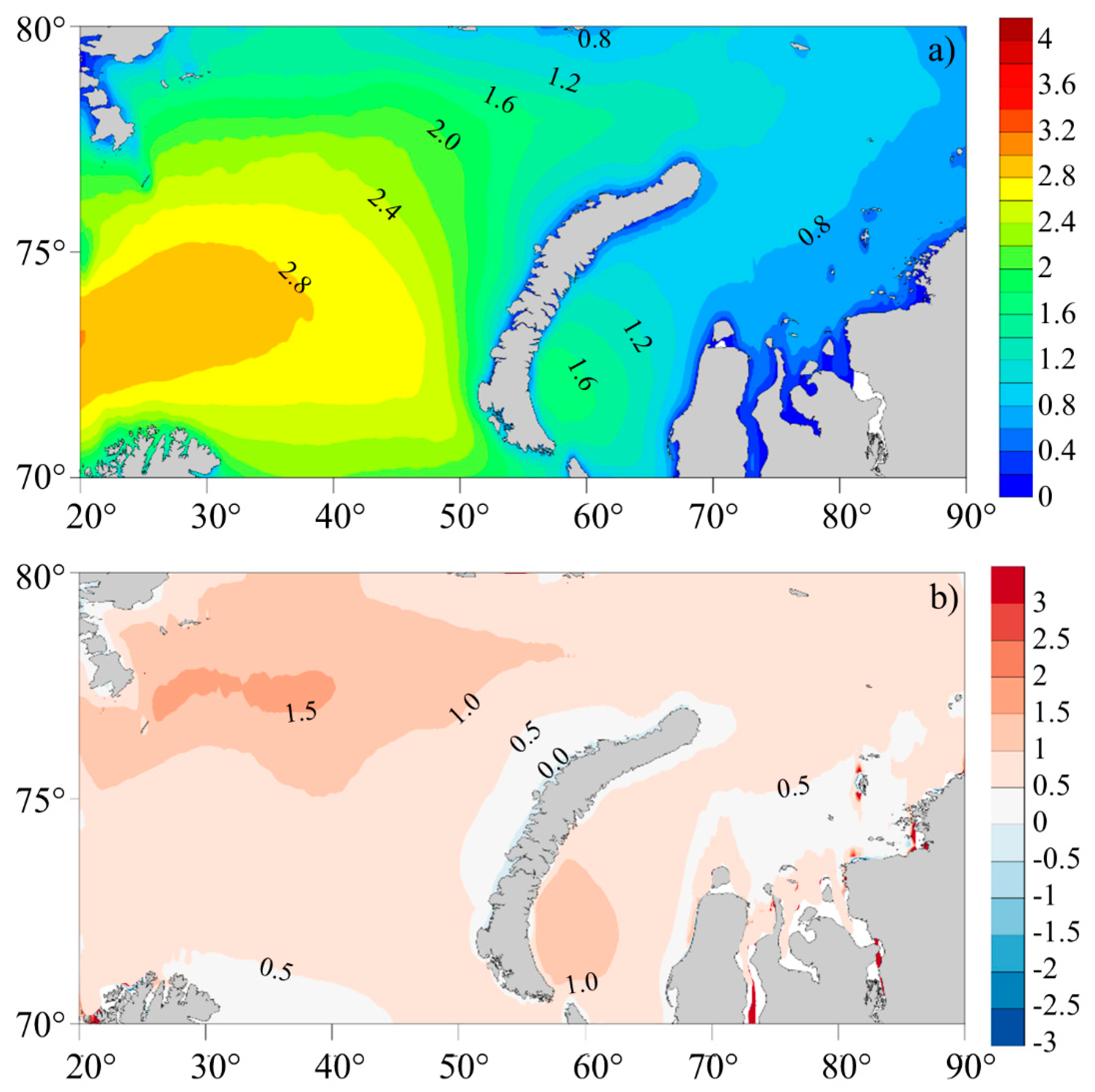
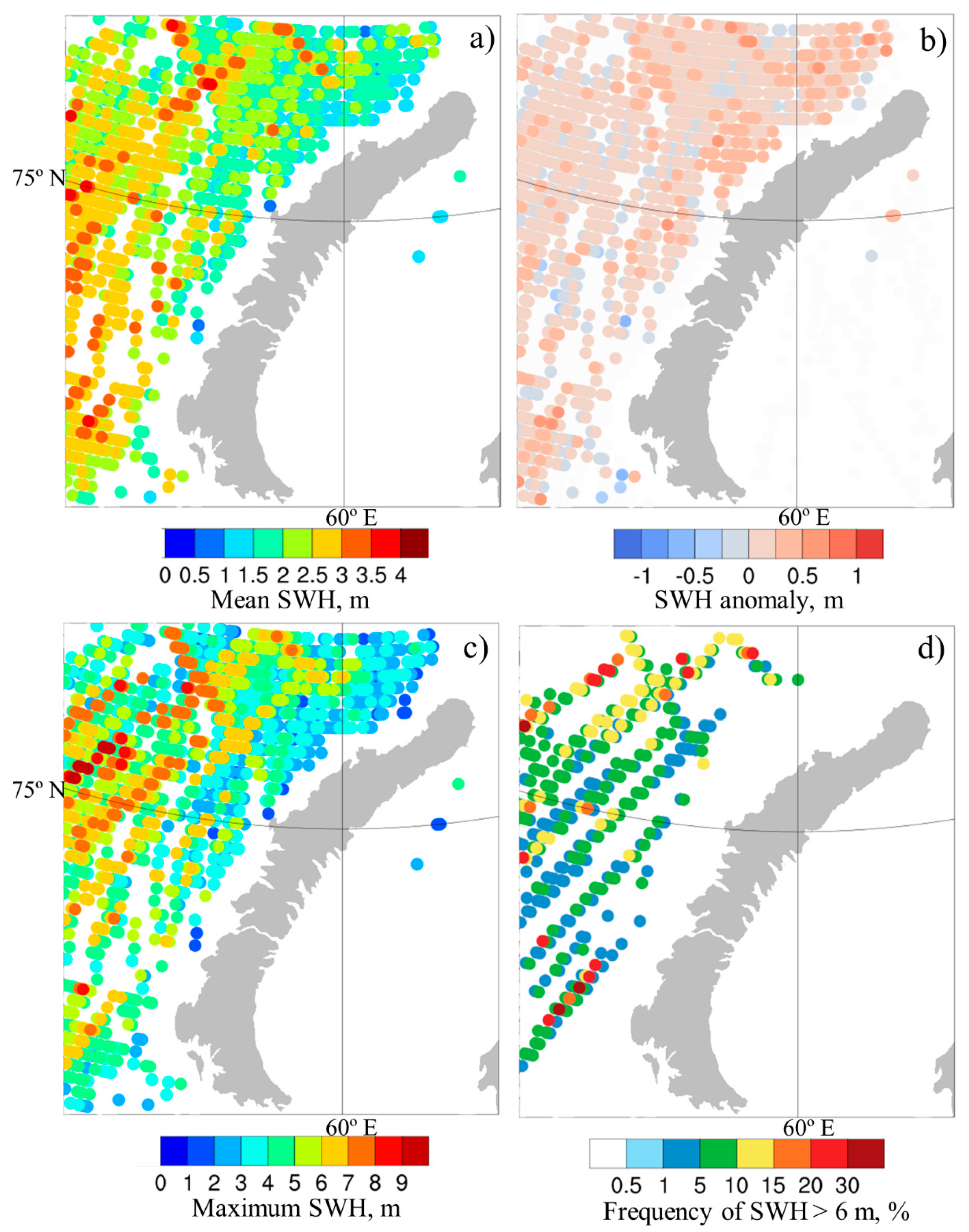
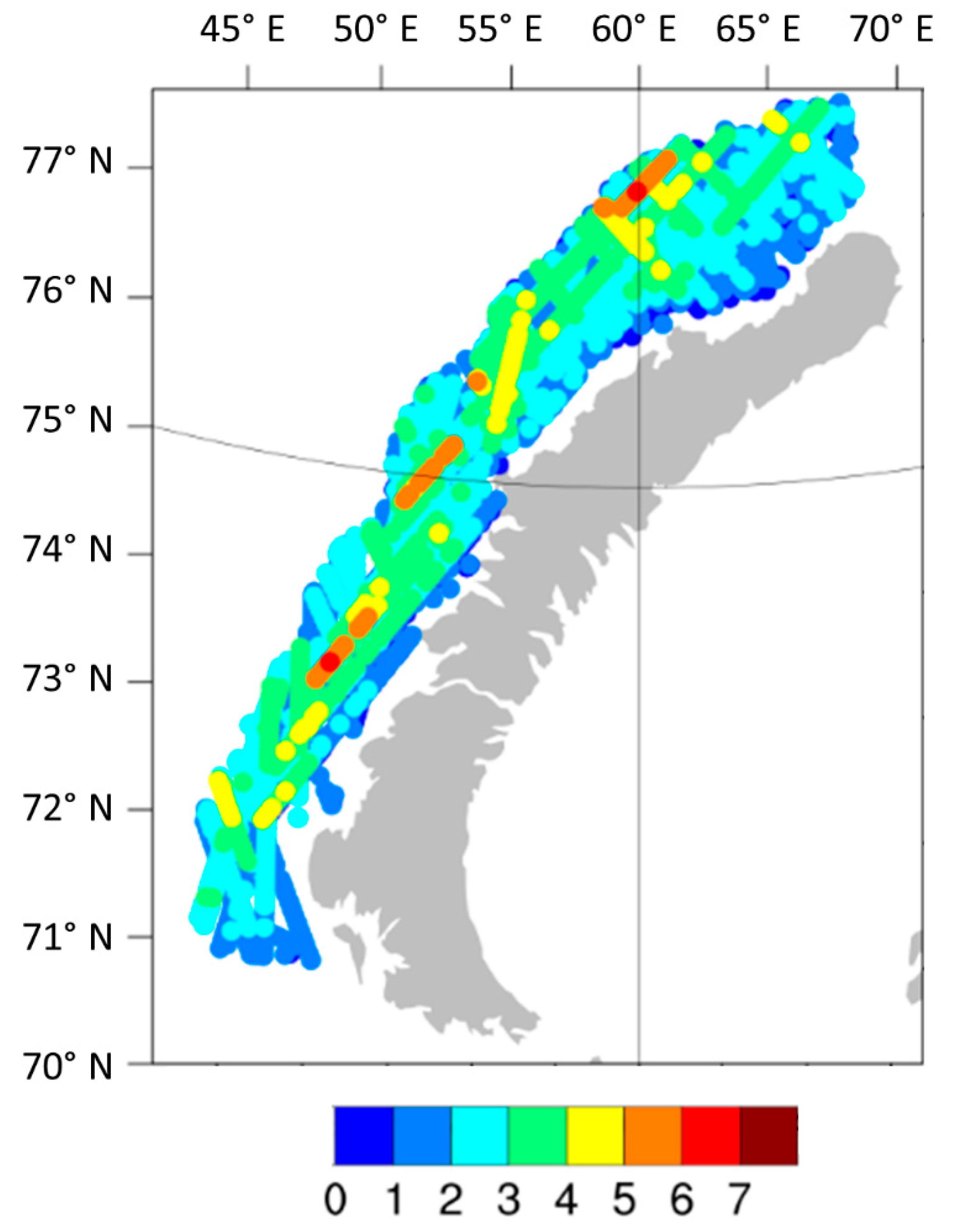
3.1. Statistics of Sea Waves during Bora

Figure 5 shows the statistics of SWH during bora according to the altimeter data interpolated on a 20-km grid according to the method described in Section 2.2. According to the altimeter data, the SWH off the Novaya Zemlya coast did not exceed 2–3 m (Figure 5a) on average, which is significantly higher than the climatic value in this area [32]. The SWH anomaly (Figure 5b), calculated as altimeter data «minus» wave reanalysis, was generally low (an average of 0.11 m over the studied region). Its spatial distribution is rather chaotic (as is also the case with other statistical wave characteristics, derived from altimeter data), which is most likely due to the short sample length. However, the prevalence of a positive anomaly (up to 0.75 m) is evident off the north coast of Novaya Zemlya, at a distance of up to 150 km from the coast. In the open sea, a slight positive anomaly (up to 0.5 m) can also be observed in individual cells.
The maximum SWH (within 20-km cells) near the archipelago reached 6–7 m (Figure 5c). Frequency of waves higher than 6 m was also calculated within each 20-km cell and is shown in Figure 5d. A more detailed analysis of cases where high waves were observed showed that such waves were mainly associated with large-scale amplification of the wind, primarily in the southern direction (when storm cyclones passes the study area). Waves of 6 m height or more were observed closest to the coast off the Matochkin Shar Strait and the northern part of the archipelago.
Figure 6 shows all of the altimeter data (5352 in total) during bora near the western coast of Novaya Zemlya, at a distance of less than 100 km from the coast. The 100 km spatial scale is characteristic for orographic winds (gap winds and bora) on the lee side of the archipelago [9,11], and one can expect to find the wave field response on this scale. Anomalies of SWH associated with bora downstream of the Northern Island of the archipelago were observed at the same distance from the coast (Figure 5b). During bora, the SWH off the coast exceeded 6 m only twice, exceeded 5 m five times, and exceeded 4 m 18 times. Moreover, waves higher than 4 m were observed at a distance of more than 40 km from the coast, and those higher than 5 m, at a distance of more than 60 km. Such a relatively small frequency of high waves is due to a short fetch and a rapid decrease in velocity of gap winds, and especially bora downstream from the coast.
Waves of 5–6 m height are often observed in the Barents Sea, being usually associated with western storms [32]. The maximum wave height for the studied region was 9–10 m according to the wave reanalysis, which was significantly higher than that during bora. Thus, the altimeter observations showed low repeatability of high waves potentially dangerous for vessels during bora.

3.2. Case Studies: Two Bora Episodes

This section discusses the results of high-resolution simulations of extreme bora episodes on 7–15 January 2006 and 9–12 February 2009 from the control experiment (ST1, see Section 2.3).
A series of storm cyclones passed through the Barents Sea in the period 7–15 January 2006; sea-level pressure in the center of the cyclones reached 955 hPa. The Novaya Zemlya region was also influenced by storm cyclones and atmospheric fronts for almost the entire episode. Mean pressure gradient was directed from west to east (Figure 7a), resulting in southerly winds over the sea. According to the altimeter data, the wind speed in the northwest of the study area reached 25 m s−1, and the SWH was 9 m.
In the period 9–12 February 2009, the weather over the Barents Sea was determined by one vast cyclone with its center located between Svalbard and the Scandinavian Peninsula (Figure 7b). Sea-level pressure pattern was close to the mean pressure composite during high-speed southeasterly winds over the Barents Sea [10]. An east–southeast wind prevailed over Novaya Zemlya and the eastern part of the sea. According to altimeter data available for 11–12 February, the wind reached 18 m s−1, and the SWH in the western part of the study area was 5.5 m.

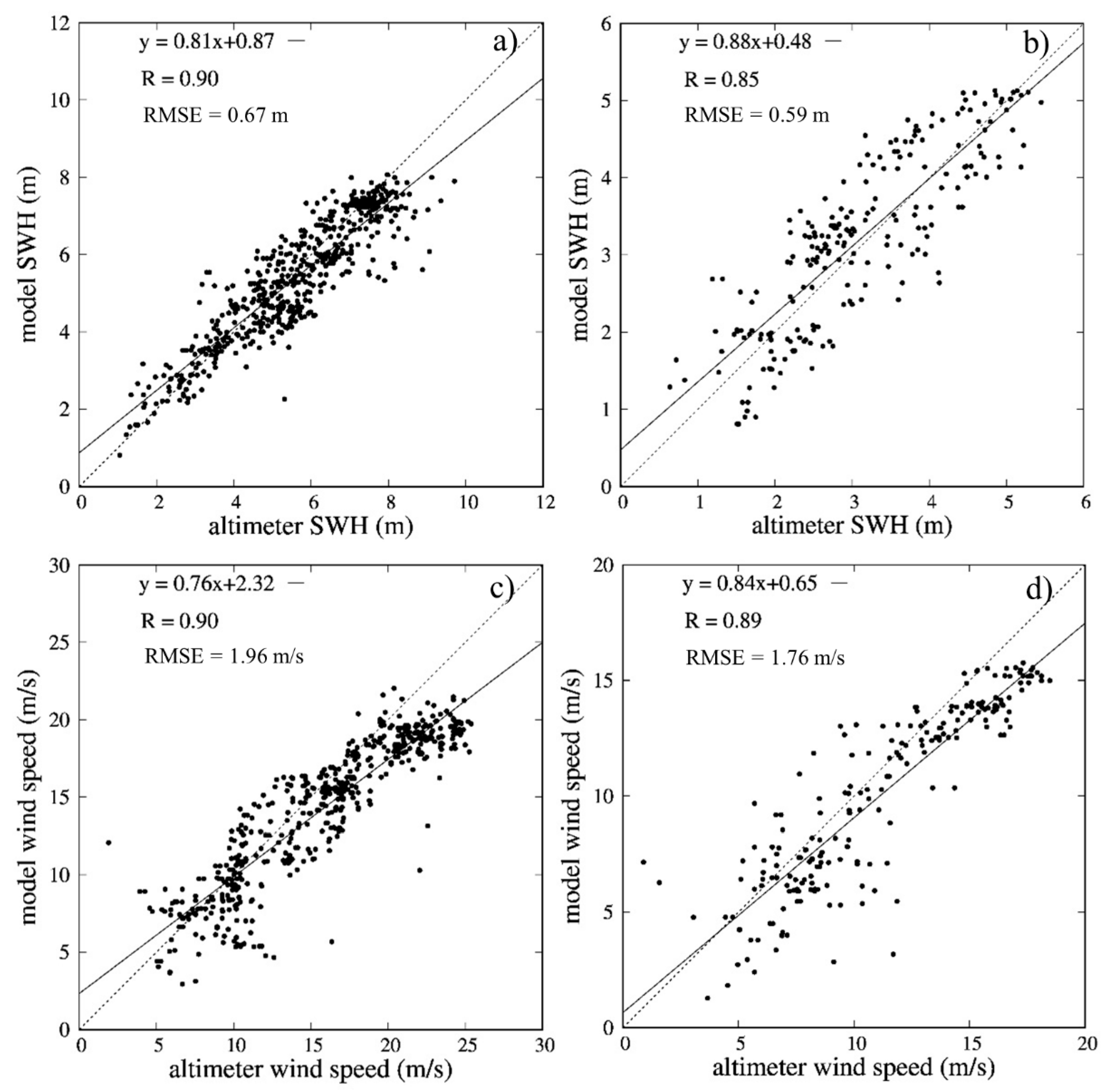
3.2.1. Model Verification

Simulated wave heights and wind speeds were verified against altimeter data (Figure 8). The average bias (model “minus” observations) of wind speed was −1.5 m s−1 in the 2006 episode and −1.1 m s−1 in the 2009 episode (i.e., within the average accuracy of altimeter measurements [31]); correlation coefficient was 0.9 in both episodes. At Malye Karmakuly station, the correlation between the model and observed wind speeds was very high, 0.95, due to observational nudging. However, the bias of wind speed at the station was much higher than that above the sea (when compared with altimeter data), which is due to a more complex mesoscale and micro-scale structure of the wind field near the mountains and a higher wind speed.
In the simulated episodes, bora-caused waves developed against the background of the preexisting swell, which was formed under the influence of cyclones moving over the Barents Sea. In such context (the development of wind waves on the background of swell), the error in wave height simulations usually increases [53]. However, even under these conditions, the quality of wave modeling in our case was rather high. The average bias of SWH was −0.2 m in the 2006 episode and 0.1 m in the 2009 episode; the correlation coefficient was 0.9 in the 2006 episode and 0.85 in the 2009 episode.

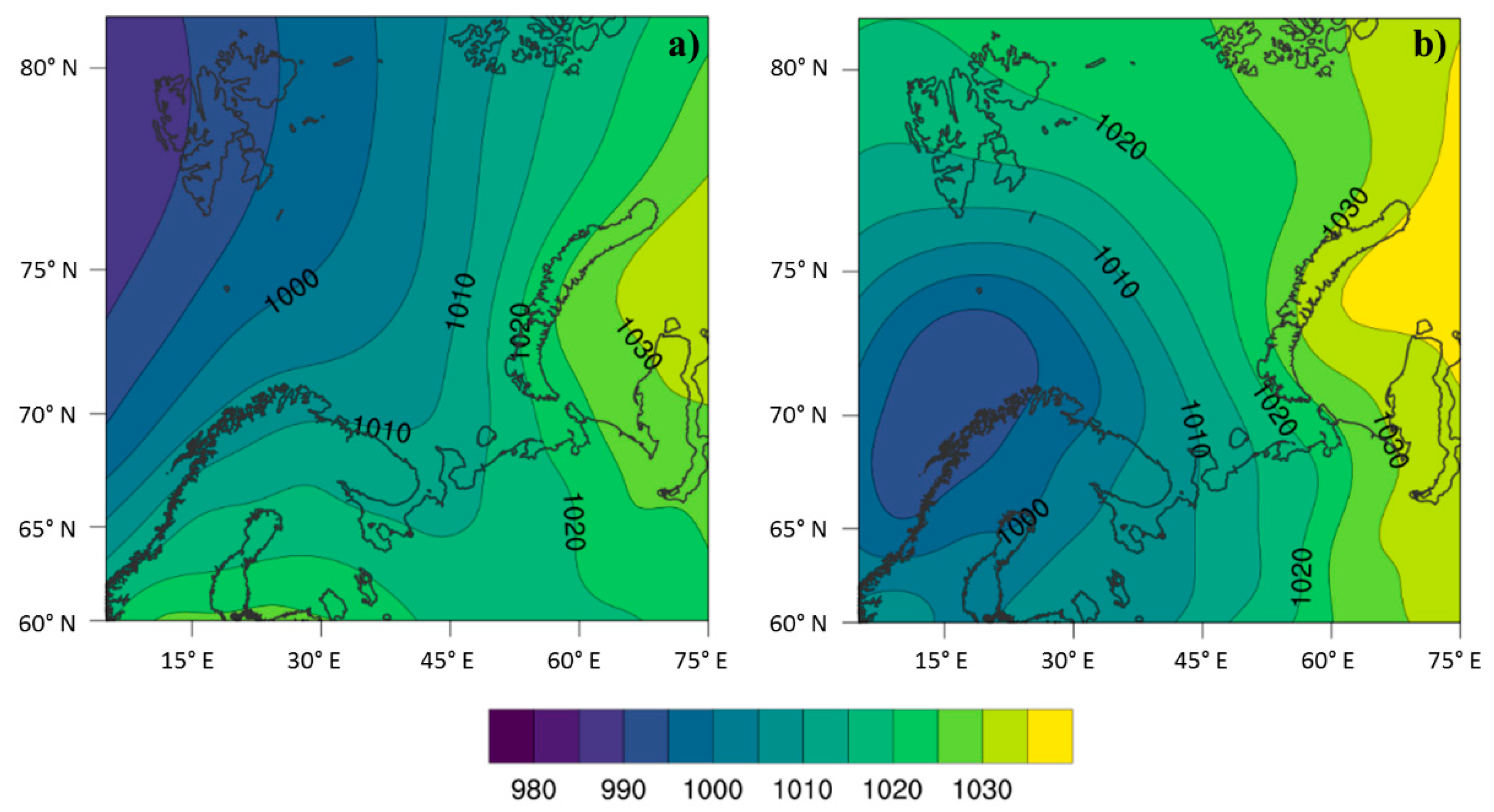
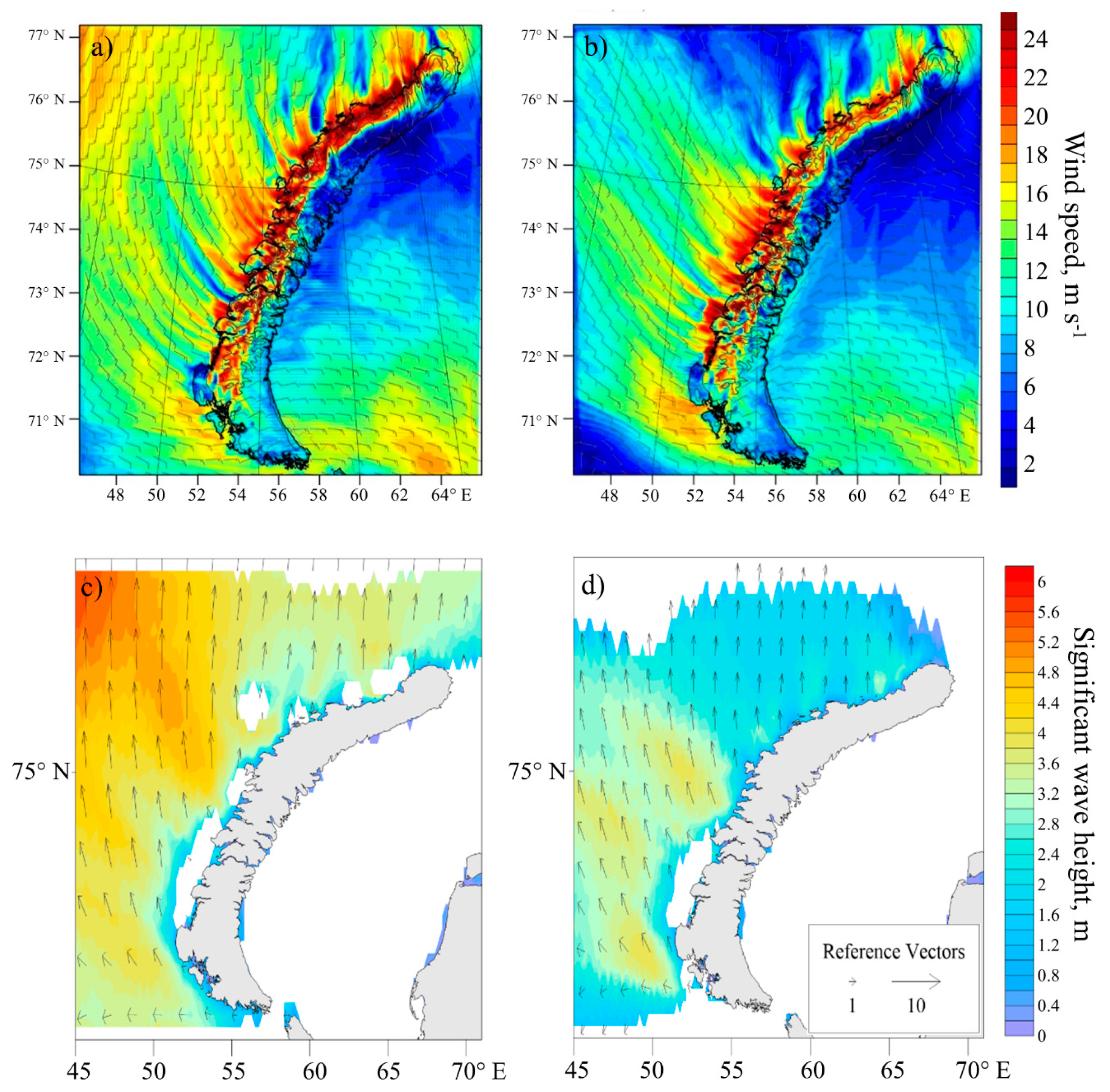
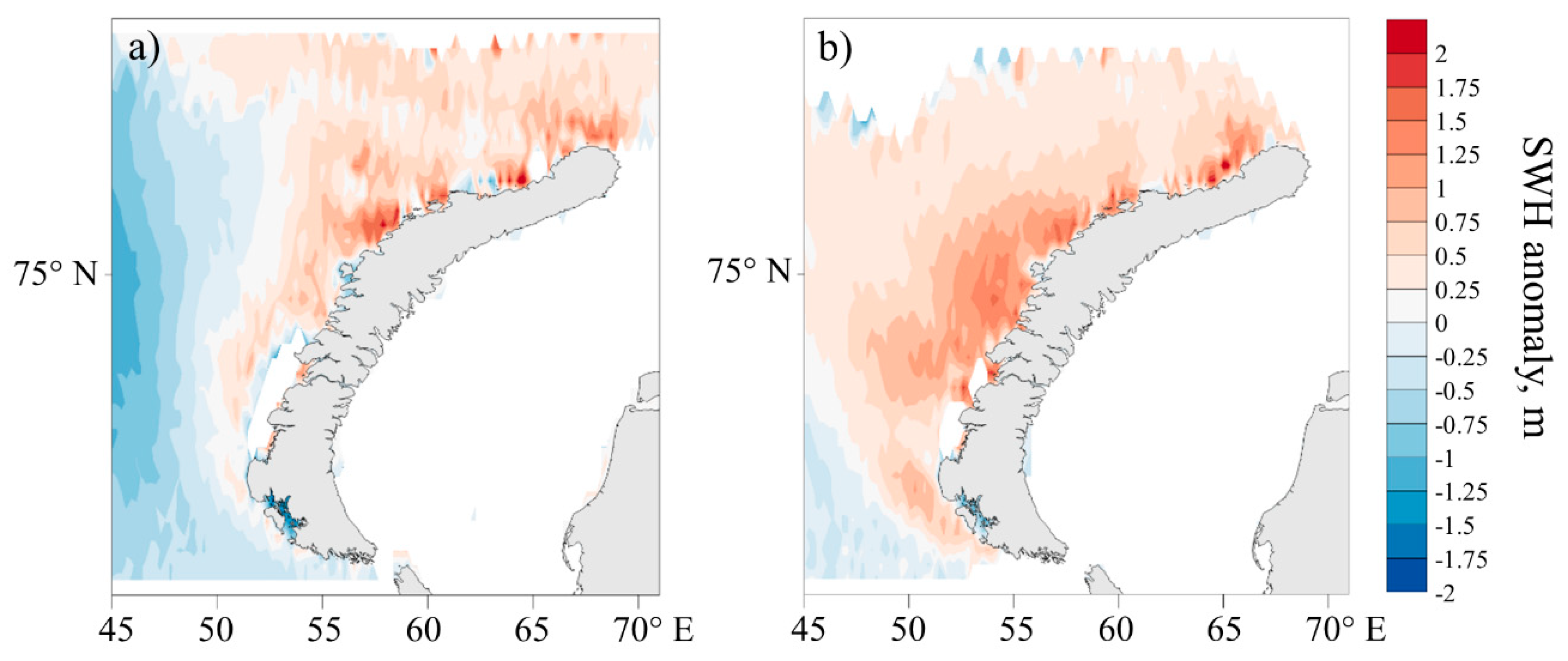
3.2.2. Bora and Sea Wave Evolution during the Episodes

In the 2006 episode, wind speed and SWH were high due to the passage of storm cyclones. At the beginning of the 2006 episode, bora was observed only in the north of the Northern Island, while it reached culmination and was clearly observed on the entire western coast of Novaya Zemlya on 12–13 January. Bora-caused waves (defined on the frequency-direction spectra as waves coming from the coast) downstream from the northern part of the archipelago were observed throughout the episode, with a small fraction of swell (with a characteristic frequency of about 0.1 Hz) (Figure 9a,c). Downstream from the central part of the archipelago, a swell prevailed in the first half of the episode (which accounted for the maximum spectral density, Figure 9b), and bora-caused waves prevailed over the swell only on 12–13 January (Figure 9d). The maximum intensity of the spectral peak of bora-caused waves was simulated in both regions on 12–13 January. In the second half of the episode, bora-caused waves became longer, with the spectral peak shifting from 0.2 to 0.1–0.15 Hz. Near the southern part of the archipelago, past ice was observed throughout the episode.
In the 2009 episode, a swell coming from the southwest (Figure 9e,f) caused by the background south and southeast wind that prevailed at the beginning of the episode was also simulated. On February 11, the background wind began to subside (causing the height of the waves in the open sea to decrease), while at the same time, the bora intensified along the entire coast, creating local maximums of wave height. Until February 12, there were two peaks of spectral density in the wave spectrum at both points A and B, for waves from the southeast and from the southwest (Figure 9e,f). Waves from the southwest with lower frequency can represent not only swell from the open sea, but also waves coming from neighboring “jets”. The alternation of high-speed jets and wakes is characteristic of orographic winds including that on Novaya Zemlya (see Figure 10). However, a swell from the open sea is still a more significant source of southwestern waves, since these waves are absent in the spectrum at the end of the episode (Figure 9g,h), while jets and wakes were observed throughout the episode. The intensity of the bora-caused waves’ spectral peak reached its maximum.
In both episodes and at both points, the spectral peak of the bora-caused waves formed rather fast and clearly appeared at the end of the first day of the experiment.

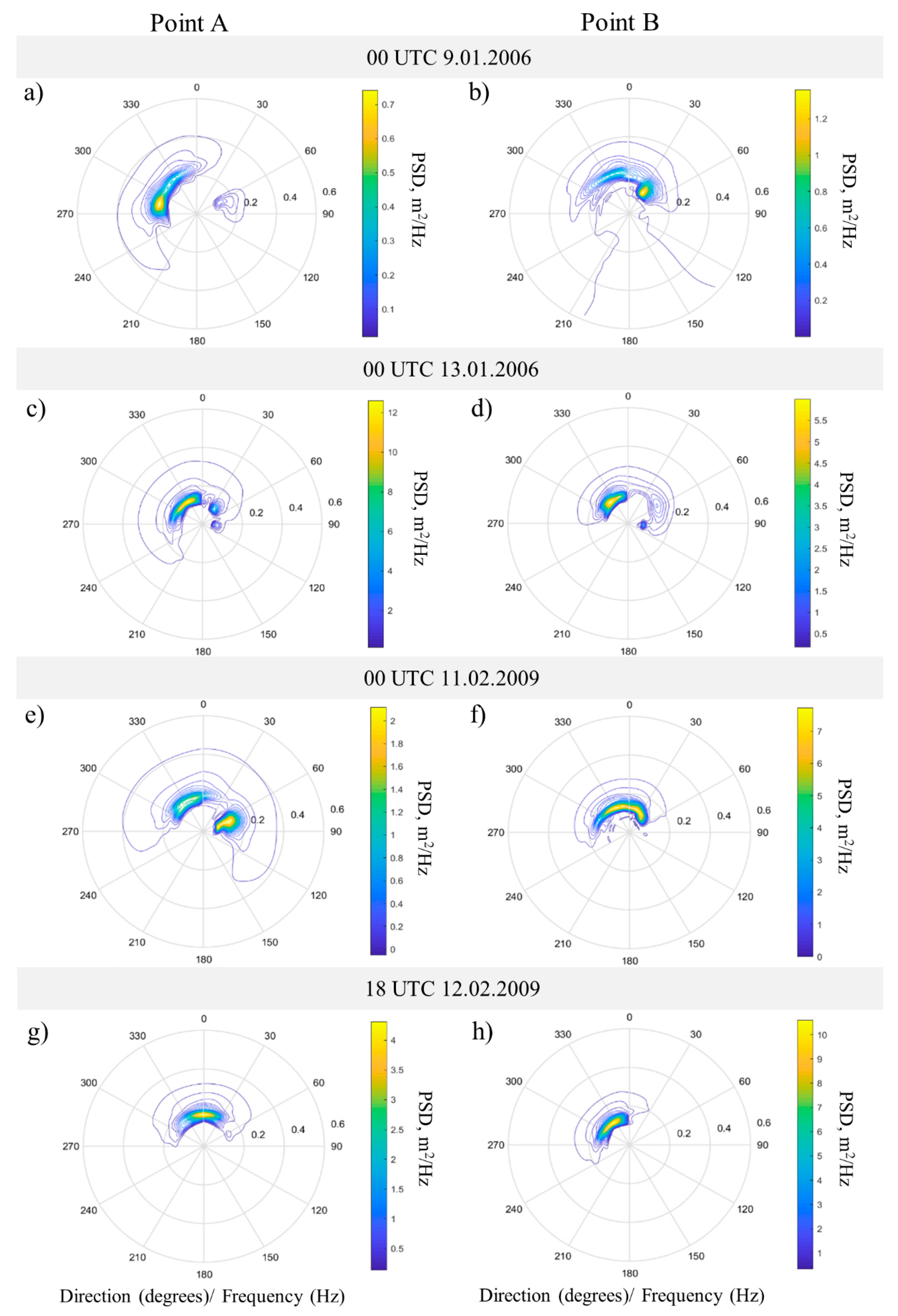
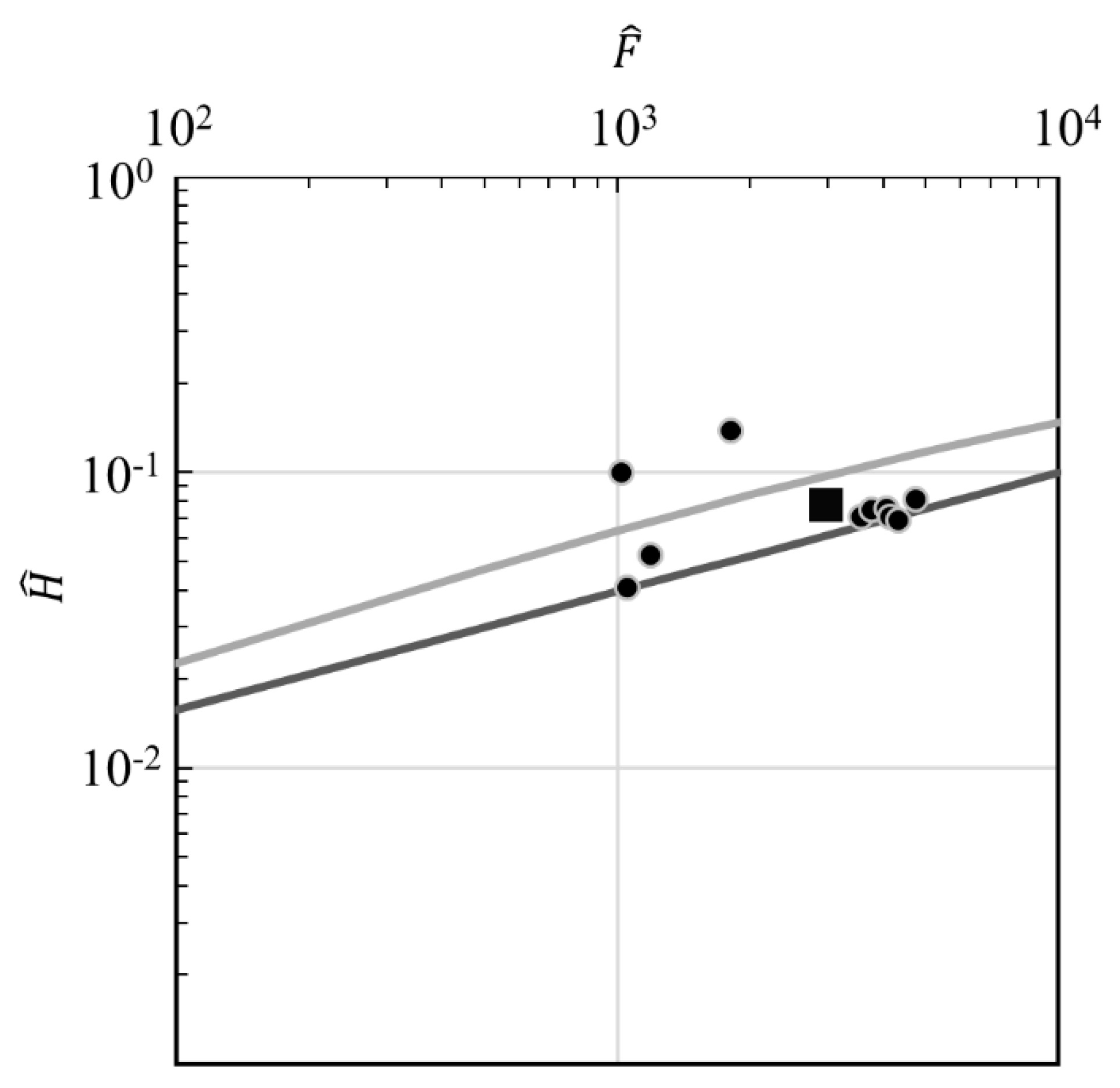
3.2.3. Features of Bora-Caused Waves

When looking at the sea wave features during bora, it is important to determine which waves are caused directly by bora. In addition to the analysis based on frequency-direction wave spectra, the effect of bora on sea waves can also be determined on the basis of the wave height anomaly. The average wave height anomaly was calculated as the wave height difference between the high-resolution simulation and wave reanalysis data (for each high-resolution model grid node the closest wave reanalysis grid node was found) and is shown in Figure 11 for both episodes. In the 2006 episode, the influence of bora on the wave field (i.e., a positive anomaly in wave height) off the southern and central parts of the archipelago propagated significantly less (approximately 100 km from the coast) than in the 2009 episode, where the absolute values of wave height were less. In the 2009 episode, the presence of bora led to a wave height increase at a distance of more than 200 km from the coast. This means that bora affects sea waves not only in the area of direct wind forcing, but also at a considerable distance from it. The anomaly map shows that in the 2006 episode the high waves in the west of the study area were caused solely by the background (large-scale) wind. Influence of bora has led to a decrease in the wave height in this region compared to the wave reanalysis. This is due to the weakening of the background southeast wind over the open sea when the Novaya Zemlya topography is well resolved in the high-resolution experiment. Downstream from the northern part of the archipelago, bora led to an increase in the wave height at a great distance, up to the ice edge. Obviously, the greatest average anomaly was simulated in coastal regions; the mean anomaly was up to 2.5 m while in some instances, it reached 3.3 m. Thus, the wave height anomaly during bora in the simulated episodes was several times higher than the average anomaly determined on the basis of the altimeter data (Section 3.1).
Now, we consider the features of sea waves in those regions where the wave height anomaly is positive (i.e., in the region of bora influence).
Figure 10 shows the times when the bora reached its culmination and sea waves near the west coast were largely influenced by bora, which was proven by the wave spectra (Figure 9c,d,g,h).
Local SWH maxima were more pronounced in the 2009 episode (although they also appeared in the 2006 episode): three elongated areas with a SWH of 3–4 m (in 2009 episode) and 4–5 m (in 2006 episode) downstream of the southern and central parts of the archipelago and less intense local maxima with a height of up to 3.5 m (2009 episode) and up to 4 m (2006 episode) downstream of the northern part of the archipelago (Figure 10c,d). In the 2009 episode, SWH up to 3 m was noted at a distance of 30 km from the coast and those up to 4 m, at a distance of about 80–90 km from the coast downstream from the central part of the archipelago; the SWH reached a maximum at a distance of 40–50 km from the coast in the north of the archipelago. In contrast to the 2009 episode, SWH continuously increased with distance from the coast in the 2006 episode. The fastest wave growth occurred downstream from Krestovaya Bay (see Figure 3a), one of the most deep-cut fjords in Novaya Zemlya. In this area, a strong gap flow propagates up to 200 km from the coast (Figure 10a,b), which is consistent with the estimates made by Ivanov [20].
SWH in the open sea is significantly lower downstream from the northern part of the archipelago than that downstream from the southern and central parts, particularly in the 2009 episode (Figure 10c,d). The jets of gap flows there had a more local character, and the bora itself almost failed to extend from the foot of the mountain ridge. This is due to the peculiarities of the flow over the ridge: the flow non-linearity also increased with the increase in topography height from the south to north (see Figure 3a). Nonlinearity of flow over obstacle is characterized by the Froude number F r = U / N h (where U and N are the wind speed and Brunt-Vaisala frequency in the incoming flow, respectively; h is the mountain ridge height), in other words, by the ratio between incoming flow and topography characteristics. The highly nonlinear flow regime (with a small Froude number) is characterized by blocking (stagnation) of the flow on the windward side of the mountains (clearly seen on Figure 10a,b) and the occurrence of the so-called hydraulic jump when the wind speed on the lee side decreases sharply [19]. Nonlinear flow is more typical for the 2009 episode, when the background wind speed was lower (and therefore the Froude number was smaller) than in the 2006 episode, which led to a stronger blocking of the flow on the windward side and a sharper velocity decrease on the lee side of Novaya Zemlya (Figure 10b).
In simplified one-dimensional and stationary approaches, the wave height during offshore wind is determined only by the fetch length (so-called fetch law) [15,54,55]. In this case, the dimensionless wave height H ^ = g H s / U 2 and the dimensionless fetch F ^ = g F / U 2 (where F is fetch length) are related by dependencies obtained from observations, for example, in [15]. Altimeter measurements of SWH off the coast (up to 100 km from the coast) downstream from the northern part of Novaya Zemlya in the 2009 episode allowed us to calculate H ^ and F ^ using the average wind speed along the fetch from the simulation results (similar to [54]). Indeed, most of the calculated points in Figure 12 lie between two empirical curves (Equation (2) and Equation (4) from [15]), which means that the development of waves during bora is mostly due to the empirical fetch laws obtained in other regions and for other conditions. However, as for other orographic winds, characterized by a combination of jets and wakes, the problem ceases to be one-dimensional. This can be seen in the example of two points in Figure 12, which stand out of two empirical curves. Altimeter observations at these two points were carried out at the boundary between the jet and wake. At this time and in previous periods, sea waves propagate not only from the coast, but also from the south, mainly from other jets situated in the central part of the archipelago. This wave behavior is described in [21]: with a combination of jets and wakes between them, waves in wakes propagate from different directions, (i.e., from neighboring jets). Therefore, the real fetch of the waves is much higher than that estimated from the distance to the coast.
Bora-caused waves in both episodes were characterized by a considerable steepness (Figure 13), which reached its maximum near the coast, which is characteristic of strong winds and short fetches. The greatest average wave steepness in both episodes was 0.045 and was observed in bays and fjords in the central and northern parts of the archipelago. In the 2009 episode, steep waves were also observed downstream from the Malye Karmakuly station. Local maxima of wave steepness coincided with areas with high wind speed from 25 to 35 m s−1. The steepness approached the threshold of wave breaking, which is usually estimated from 1/7 to 1/20 [56]. The Novaya Zemlya bora is known to be the cause of poor visibility due to blizzards and spray [4]. The latter is most likely ejected into the atmosphere during the wave breaking.

3.3. Impact of Wind Input Parametrizations on Modeling Results

Figure 14 and Figure 15 show the influence of various wind input parameterization on the results of wave simulation. The experiment modified for short fetches (ST1_mod) and experiment ST6 reproduced significantly higher SWH than the control experiment. SWH in both episodes reached 5–6 m right at the coast in the central and northern parts of the archipelago (Figure 14). In contrast to the control experiment, SWH gradually decreased from the coast further downstream. SWH in the open sea was higher in the ST6 experiment than in other experiments, while SWH increased more locally, only near the coast, in the ST1_mod experiment. Waves near the coast were formed mainly under the influence of wind with the speed of 25 m s−1, which corresponded to the region of the intersection of C D U 10 dependencies in the ST1_mod and ST6 experiments (see Figure 4). This explains the similarity of the simulation results in the coastal zone. At the same time, higher SWH offshore, where the wind weakened, in experiment ST6 can be explained by a higher C D (compared with experiment ST1_mod) (Figure 4).
The average wave steepness in the ST6 and ST1_mod experiments (Figure 15) slightly decreased in comparison with the control experiment (Figure 13), especially in the open sea. This is due to a decrease in the peak wave frequency in the ST6 and ST1_mod experiments both near the coast and in the open sea (not shown). In turn, the decrease in the peak wave frequency was caused by the faster development of waves in the ST6 and ST1_mod experiments, and due to nonlinear interactions, the spectral peak shifted faster to the low-frequency range. Consequently, the wavelength at the wave spectral peak increased and the steepness decreased.
Table 1 shows a comparison of the SWH between the altimeter data and experiments with various wind input parameterizations. On average, the control experiment (ST1) was closer to the altimeter observations than the ST1_mod and ST6 experiments, which was especially evident in the 2009 episode. Model bias in the control experiment was almost an order of magnitude smaller than that in the ST6 experiment in the 2009 episode. However, a comparison was carried out at a distance of more than 20 km from the coast, where the effect of short fetches and the influence of bora were not as great as near the coast.
Figure 16 shows the spatial distribution of modeling errors (only the 2009 episode is shown). The ST1_mod and ST6 experiments substantially overestimated the SWH compared to the altimeter data and control experiment downstream of the northern part of the archipelago at a distance of 20–100 km from the coast, especially in the 2009 episode. Frequency-direction wave spectra showed that bora-caused waves (i.e., coming from the coast) predominated in this region (point A, Figure 9). Their height was substantially overestimated in the ST6 and ST1_mod experiments due to faster wave growth. At the same time, there was a tendency to underestimate (stronger than in other experiments) the SWH downstream from the central and southern parts of the archipelago in the ST1_mod experiment.

4. Summary and Conclusions

An analysis of the Novaya Zemlya bora impact on sea waves was carried out for the first time using all data sources available in the region: satellite altimeter data, wave reanalysis, and high-resolution numerical simulation. The main conclusions are as follows.
1. According to the satellite altimeter data, the average SWH during bora was higher than the climatology of SWH, but the frequency of high waves at a distance of up to 100 km from the coast was very small; waves with SWH > 6 m were recorded only twice in 5352 observations. Such a low frequency of high waves is associated with short fetches: areas of strong wind during bora and gap winds usually do not propagate far from the coast, although the influence of individual jets can be traced up to 200 km from the coast.
Numerical experiments with the WW3 and WRF-ARW models confirmed the altimeter-data-based conclusions on the low frequency of high waves during bora. SWH caused by bora did not exceed 5 m, even for prolonged and strong wind forcing (wind speed > 30 m s−1) due to limited fetch. Nevertheless, a SWH of 3–4 m was noted at a relatively short distance from the coast (which was confirmed by the altimeter data, see Figure 6). In such a case, the maximum wave height, which can be roughly estimated as 2Hs [56], is 6–8 m, which poses hazards to navigation near the coasts.
2. According to the altimeter data, the SWH anomaly related to bora and gap winds were small on average (up to 0.75 m downstream from the northern part of the archipelago). However, numerical modeling revealed a SWH anomaly of 2–3 m near the coast in some cases of severe bora, which is up to 100% of SWH near the coast. This magnitude of the anomaly significantly exceeds the order of magnitude of RMSE of the wave height forecasts, usually estimated as 10−1 m (e.g., [57,58]). When the wave field is not strongly influenced by the large-scale circulation (e.g., the passage of a series of storm cyclones), the influence of bora extends over a large distance from the coast (more than 200 km), as in the 2009 episode.
In addition to errors in the wave forecast, neglecting the bora can lead to erroneous forecasting of other processes associated with waves such as mixing of the upper layer of the ocean and atmosphere–ocean turbulent heat transfer. Sea waves affect the turbulent fluxes through the roughness parameter z 0 . Using the well-known parametrizations of z 0 , with sea waves taken into account, one can approximately estimate an error in determining the roughness parameter caused by underestimating the wave height during bora. For example, the difference in roughness parameter for different wave heights (all other conditions being equal) in the widely used parameterization of Taylor and Yelland [59] can be written as Δ z 0 = a / L b H s 1 b + 1 H s 2 b + 1 , where Hs1 is the wave height according to high-resolution modeling (when bora is taken into account) and Hs2 is the wave height according to wave reanalysis (without bora), L is the wavelength, a = 1200, b = 4.5. The magnitude of Δ z 0 calculated in the area influenced by bora is on average about 10−3–10−2 m in both episodes, which is comparable with the magnitude of z 0 above the sea in moderate to strong winds (e.g., [60]). Due to the high frequency and intensity of the Novaya Zemlya bora [2], its effect on the sea waves and related processes can lead to appreciable climate response.
Accurate accounting for the heat and momentum exchange on the surface is important not only for climate tasks, but also for weather forecasting. The resolution of modern numerical weather prediction models (~10 km) still does not allow us to correctly reproduce the spatial structure of bora winds and associated waves, and the extreme values of wind speed (and therefore wave height) are usually underestimated by models [37,61]. When averaging over a large space or long time period, differences in wind speed, heat, and momentum fluxes between high- and low-resolution models are likely to be small [37]. However, it is still unknown how the incorrect spatial distribution and underestimation of the maximum wind speed will affect the forecast quality including that in remote regions. The problem of the influence of an unresolved momentum due to bora wind and waves on the forecast skill, in contrast to the more studied (and parameterized) influence of other orographic effects such as flow blocking, gravity waves, and orographic turbulence [62,63], has not been properly investigated. More or less realistic energy exchange between the atmosphere, ocean, and sea waves during bora could be obtained using the coupled modeling, which should be the next step in the investigations into the Novaya Zemlya bora and other orographic winds.
3. Some features of the bora-caused waves were investigated on the basis of simulations of two episodes of severe bora. An increase in SWH under the influence of bora and gap winds can be traced at a great distance from the coast downstream from the central part of the archipelago, cut up by numerous glacial valleys and passes. The most rapid wave growth is also noted in this region, where intense and far-spreading gap winds blow. The influence of bora and gap winds does not extend so far downstream of the northern part of the archipelago, where the height of the mountain ridges is greater. There, the influence of bora on the wave field is more local, and the maximum wave height is noted to be closer to the coast.
Using simulation results and altimeter data, we showed that the standard fetch laws do not strictly apply during bora due to the peculiarities (strong spatial heterogeneity) of wind forcing. The combination of wind waves coming from the shore, caused by bora, and swell from the open sea and from the neighboring jets should lead to significant three-dimensionality of the waves. Confused state of the sea arising in such a case increases risks to vessel stability [64]. The average wave steepness during bora is large and, according to the control experiment, reached 0.045 (i.e., an order of magnitude higher than the threshold value for very steep waves [42]. Thus, bora-caused waves pose a hazard for vessels not only due to their height, but also due to confusion, steepness, and short periods of the waves, which are especially unfavorable factors for small crafts [64].
The wave field during bora soon adapts to wind forcing. The correlation coefficient of SWH and wind speed in coastal areas did not exceed 0.9 (not shown), and the spectral density peak of bora-caused waves already appeared on the spectrum at a distance of 40 km from the coast on the first day of the numerical experiments.
4. As expected, the height of the waves in the experiment, taking into account short fetches, increased in comparison with the control experiment. However, a comparison with the satellite altimeter data showed that at distances of at least 20 km from the coast or more, where observational data were available for simulated episodes, experiments with the ST1_mod and ST6 parameterizations were more biased than the control experiment (with ST1 parameterization). However, the question of the suitability of different wind input parametrizations directly at the shore, where the influence of bora is greatest, remains open.

Author Contributions

Conceptualization, A.A.S.; Methodology, S.A.M. and A.M.K.; Formal analysis, A.A.S., S.A.M., and A.M.K.; Writing—original draft preparation, A.A.S., S.A.M., and A.M.K. All authors have read and agreed to the published version of the manuscript.

Funding

This work was funded by the Russian Foundation for Basic Researches, grants NO 18-05-80065 (creating bora calendar, satellite data analysis), 18-05-60083 (creating wave reanalysis, high-resolution wave modeling), and 18-05-60299 (wave modeling with modified wind input parametrization).

Conflicts of Interest

The authors declare no conflicts of interest.

References

  1. Vize, V.Y. The Novaya Zemlya bora. Izv. Tsentr. Gidrometeorol. Byuro 1925, 5, 1–55. (In Russian) [Google Scholar]
  2. Shestakova, A.A.; Toropov, P.A.; Matveeva, T.A. Climatology of extreme downslope windstorms in the Russian Arctic. Weather Clim. Extrem. 2020, 28, 100256. [Google Scholar] [CrossRef]
  3. Samuelsen, E.M.; Graversen, R.G. Weather situation during observed ship-icing events off the coast of Northern Norway and the Svalbard archipelago. Weather Clim. Extrem. 2019, 24, 100200. [Google Scholar] [CrossRef]
  4. Pastusiak, T. Northern Sea Route as a Shipping Lane; Springer: New York, NY, USA, 2016; p. 219. [Google Scholar]
  5. Buzin, I.V.; Glazovskiy, A.F. Icebergs of shokalsky glacier, Novaya Zemlya. Mater. Glaciol. Res. 2005, 99, 39–44. (In Russian) [Google Scholar]
  6. Langodan, S.; Cavaleri, L.; Viswanadhapalli, Y.; Hoteit, I. The Red Sea: A natural laboratory for wind and wave modeling. J. Phys. Oceanogr. 2014, 44, 3139–3159. [Google Scholar] [CrossRef] [Green Version]
  7. Toropov, P.A.; Myslenkov, S.A.; Shestakova, A.A. Numerical simulation of Novorossiysk bora and related wind waves using the WRF-ARW and SWAN models. Russ. J. Earth Sci. 2012, 12. [Google Scholar] [CrossRef]
  8. Shestakova, A.A.; Repina, I.A. Overview of strong winds on the coasts of the Russian Arctic seas. Ecol. Montenegrina 2019, 25, 14–25. [Google Scholar] [CrossRef]
  9. Bryazgin, N.N.; Dementiev, A.A. Hazardous Meteorological Phenomena in the Russian Arctic; Gidrometeoizdat: Sankt-Petersburg, Russia, 1996; p. 150. (In Russian) [Google Scholar]
  10. Moore, G.W.K. The Novaya Zemlya Bora and its impact on Barents Sea air-sea interaction. Geophys. Res. Lett. 2013, 40, 3462–3467. [Google Scholar] [CrossRef] [Green Version]
  11. Ivanov, A.Y. Novaya Zemlya Bora and Polar Cyclones Visible from Space in Radar and Optical Imagery. Issled. Zemli Kosm. 2016, 4, 9–22. (In Russian) [Google Scholar] [CrossRef]
  12. Shestakova, A.A. The Novaya Zemlya bora: The downwind characteristics and the incomming flow structure. Arct. Antarct. 2016, 2, 86–98. (In Russian) [Google Scholar] [CrossRef]
  13. Efimov, V.V.; Komarovskaya, O.I. The Novaya Zemlya Bora: Analysis and Numerical Modeling. Izv. Atmos. Ocean. Phys. 2018, 54, 73–85. [Google Scholar] [CrossRef]
  14. Shestakova, A.A.; Moiseenko, K.B. Hydraulic regimes of flow over mountains during severe downslope windstorms: Novorossiysk bora, Novaya Zemlya bora, and Pevek Yuzhak. Izv. Atmos. Ocean. Phys. 2018, 54, 344–353. [Google Scholar] [CrossRef]
  15. Wilson, B.W. Numerical prediction of ocean waves in the North Atlantic for December, 1959. Dtsch. Hydrogr. Z. 1965, 18, 114–130. [Google Scholar] [CrossRef]
  16. Golubkin, P.A.; Kudryavtsev, V.N.; Chapron, B. On wind wave development in the Arctic seas based on AltiKa altimeter measurements. Sovrem. Probl. Distancionnogo Zondirovaniya Zemli Kosm. 2017, 14, 179–192. (In Russian) [Google Scholar] [CrossRef]
  17. Skeie, P.; Grønås, S. Strongly stratified easterly flows across Spitsbergen. Tellus A Dyn. Meteorol. Oceanogr. 2000, 52, 473–486. [Google Scholar] [CrossRef]
  18. Shestakova, A.A.; Toropov, P.A.; Stepanenko, V.M.; Sergeev, D.E.; Repina, I.A. Observations and modelling of downslope windstorm in Novorossiysk. Dyn. Atmos. Ocean. 2018, 83, 83–99. [Google Scholar] [CrossRef]
  19. Durran, D.R. Another look at downslope windstorms. Part I: The development of analogs to supercritical flow in an infinitely deep, continuously stratified fluid. J. Atmos. Sci. 1986, 43, 2527–2543. [Google Scholar] [CrossRef]
  20. Ivanov, A.Y. Local katabatic winds of the Russian Federation and their observation from space using SAR imagery. Issled. Zemli Kosm. 2019, 5, 15–35. (In Russian) [Google Scholar] [CrossRef]
  21. Shimada, T.; Kawamura, H. Wind-wave development under alternating wind jets and wakes induced by orographic effects. Geophys. Res. Lett. 2006, 33. [Google Scholar] [CrossRef]
  22. RIHMI-WDC. Available online: http://meteo.ru/ (accessed on 3 July 2020).
  23. Golubkin, P.A.; Kudryavtsev, V.N.; Chapron, B. Wind Waves in the Arctic Seas from Satellite Altimetry Data. Issled. Zemli Kosm. 2015, 4, 25. [Google Scholar] [CrossRef]
  24. Ribal, A.; Young, I.R. 33 years of globally calibrated wave height and wind speed data based on altimeter observations. Sci. Data 2019, 6, 77. [Google Scholar] [CrossRef] [PubMed] [Green Version]
  25. AODN. Available online: https://portal.aodn.org.au/ (accessed on 3 July 2020).
  26. Janssen, P.; Abdalla, S.; Hersbsch, H.; Bidlot, J.-R. Error estimation of buoy, satellite, and model wave height data. J. Atm. Ocean. Tech. 2006, 24, 1665. [Google Scholar] [CrossRef] [Green Version]
  27. Jayaram, C.; Bansal, S.; Krishnaveni, A.S.; Chacko, N.; Chowdary, V.M.; Dutta, D.; Rao, K.H.; Dutt, C.B.S.; Sharma, J.R.; Dadhwal, V.K. Evaluation of SARAL/AltiKa Measured Significant Wave Height and Wind Speed in the Indian Ocean Region. J. Indian Soc. Remote Sens. 2016, 44, 225–231. [Google Scholar] [CrossRef]
  28. Gourrion, J.; Vandemark, D.; Bailey, S.; Chapron, B.; Gommenginger, G.P.; Challenor, P.G.; Srokosz, M.A. A two-parameter wind speed algorithm for Ku-band altimeters. J. Atmos. Ocean. Technol. 2002, 19, 2030–2048. [Google Scholar] [CrossRef]
  29. Golubkin, P.A.; Chapron, B.; Kudryavtsev, V.N. Wind Waves in the Arctic Seas: Envisat and AltiKa Data Analysis. Mar. Geod. 2014, 38, 289–298. [Google Scholar] [CrossRef]
  30. Farjami, H.; Golubkin, P.; Chapron, B. Impact of the sea state on altimeter measurements in coastal regions. Remote Sens. Lett. 2016, 7, 935–944. [Google Scholar] [CrossRef]
  31. Lavrova, O.Y.; Kostianoy, A.G.; Lebedev, S.A.; Mityagina, V.I.; Ginzburg, A.I.; Sheremet, N.A. Complex Satellite Monitoring of the Russian Seas; IKI RAN: Moscow, Russia, 2011; p. 470. [Google Scholar]
  32. Myslenkov, S.A.; Markina, M.Y.; Arkhipkin, V.S.; Tilinina, N.D. Frequency of storms in the Barents Sea under modern climate conditions. Vestn. Mosk. Univ. Seriya 5 Geogr. 2019, 2, 45–54. (In Russian) [Google Scholar]
  33. Saha, S.; Moorthi, S.; Pan, H.L.; Wu, X.; Wang, J.; Nadiga, S.; Tripp, P.; Kistler, R.; Woollen, J.; Behringer, D.; et al. NCEP Climate Forecast System Reanalysis (CFSR) 6-Hourly Products, January 1979 to December 2010; Research Data Archive at the National Center for Atmospheric Research, Computational and Information Systems Laboratory: Boulder, CO, USA, 2010. [Google Scholar]
  34. Saha, S.; Moorthi, S.; Wu, X.; Wang, J.; Nadiga, S.; Tripp, P.; Behringer, D.; Hou, Y.-T.; Chuang, H.-Y.; Iredell, M.; et al. The NCEP climate forecast system version 2. J. Clim. 2014, 27, 2185–2208. [Google Scholar] [CrossRef]
  35. Myslenkov, S.A.; Markina, M.Y.; Kiseleva, S.V.; Stoliarova, E.V.; Arkhipkin, V.S.; Umnov, P.M. Estimation of Available Wave Energy in the Barents Sea. Therm. Eng. 2018, 65, 411–419. [Google Scholar] [CrossRef]
  36. Myslenkov, S.; Medvedeva, A.; Arkhipkin, V.; Markina, M.; Surkova, G.; Krylov, A.; Dobrolyubov, S.; Zilitinkevich, S.; Koltermann, P. Long-term statistics of storms in the Baltic, Barents and White Seas and their future climate projections. Geogr. Environ. Sustain. 2018, 11, 93–112. [Google Scholar] [CrossRef] [Green Version]
  37. Hughes, M.; Cassano, J.J. The climatological distribution of extreme Arctic winds and implications for ocean and sea ice processes. J. Geophys. Res. Atmos. 2015, 120, 7358–7377. [Google Scholar] [CrossRef]
  38. Tolman, H.L. User Manual and System Documentation of WAVEWATCHIII Version 4.18.; Technical Note; NOAA; NWS; NCEP; MMAB: College Park, MD, USA, 2014; 302p. Available online: https://polar.ncep.noaa.gov/waves/wavewatch/manual.v4.18 (accessed on 6 July 2020).
  39. Deng, X.; Featherstone, W.E.; Hwang, C.; Berry, P.A.M. Estimation of contamination of ERS-2 and POSEIDON satellite radar altimetry close to the coasts of Australia. Mar. Geod. 2002, 25, 249–271. [Google Scholar] [CrossRef]
  40. ASR v.2 Download Page. Available online: https://rda.ucar.edu/datasets/ds631.1/ (accessed on 3 July 2020).
  41. Buckley, W.H. Extreme and climatic wave spectra for use in structural design of ships. Nav. Eng. J. 1988, 100, 36–58. [Google Scholar] [CrossRef]
  42. Natinal Data Buoy Center. Available online: https://www.ndbc.noaa.gov/wavecalc.shtml (accessed on 3 July 2020).
  43. Polnikov, V.G.; Zilitinkevich, N.S.; Pogarskii, F.A.; Kubryakov, A.A. Comparative evaluation of accuracy of numerical wave models based on satellite altimetry data. Process. Geosredah 2017, 4, 700–709. (In Russian) [Google Scholar]
  44. Wu, J. Wind-stress coefficients over sea surface from breeze to hurricane. J. Geophys. Res. Ocean. 1982, 87, 9704–9706. [Google Scholar] [CrossRef]
  45. Repina, I.A.; Artamonov, A.Y.; Varentsov, M.I.; Kozyrev, A.V. Experimental study of the sea surface wind drag coefficient at strong winds. Morsk. Gidrofiz. Zhurnal 2015, 1, 53–63. (In Russian) [Google Scholar] [CrossRef] [Green Version]
  46. Kuznetsova, A.M.; Baydakov, G.A.; Papko, V.V.; Kandaurov, A.A.; Vdovin, M.I.; Sergeev, D.A.; Troitskaya, Y.I. Adjusting of wind input source term in WAVEWATCH III model for the middle-sized water body on the basis of the field experiment. Adv. Meteorol. 2016, 1, 1–13. [Google Scholar] [CrossRef] [Green Version]
  47. Kuznetsova, A.M.; Dosaev, A.S.; Baydakov, G.A.; Balandina, G.N.; Sergeev, D.A.; Troitskaya, Y.I. Adjusting of the discrete interaction approximation (DIA) nonlinear source term in WaveWatchIII model to the conditions of the middle-sized reservoir. Process. Geosredah 2018, 3, 160–258. [Google Scholar] [CrossRef] [Green Version]
  48. Kuznetsova, A.M.; Dosaev, A.S.; Baydakov, G.A.; Sergeev, D.A.; Troitskaya, Y.I. Adaptation of the Nonlinear Wave-Wave Interaction Parameterization for the Short Fetches Conditions in the Wave Prediction Model WAVEWATCH III. Izv. Ross. Akad. Nauk Fiz. Atmos. Okeana 2020, 56, 224–233. (In Russian) [Google Scholar] [CrossRef]
  49. Rogers, W.E.; Babanin, A.V.; Wang, D.W. Observation-consistent input and whitecapping dissipation in a model for wind-generated surface waves: Description and simple calculations. J. Atmos. Ocean. Technol. 2012, 29, 1329–1346. [Google Scholar] [CrossRef]
  50. Zieger, S.; Babanin, A.V.; Rogers, W.E.; Young, I.R. Observation-based source terms in the third-generation wave model WAVEWATCH. Ocean Model. 2015, 96, 2–25. [Google Scholar] [CrossRef] [Green Version]
  51. van Vledder, G.P.; Hulst, S.T.C.; McConochie, J.D. Source term balance in a severe storm in the Southern North Sea. Ocean Dyn. 2016, 66, 1681–1697. [Google Scholar] [CrossRef] [Green Version]
  52. Liu, Q.; Rogers, W.E.; Babanin, A.V.; Young, I.R.; Romero, L.; Zieger, S.; Qiao, F.; Guan, C. Observation-based source terms in the third-generation wave model WAVEWATCH III: Updates and verification. J. Phys. Oceanogr. 2019, 49, 489–517. [Google Scholar] [CrossRef]
  53. Bolaños, R.; Sánchez-Arcilla, A. A note on nearshore wave features: Implications for wave generation. Prog. Oceanogr. 2006, 70, 168–180. [Google Scholar] [CrossRef]
  54. Isoguchi, O.; Kawamura, H. Coastal wind jets flowing into the Tsushima Strait and their effect on wind-wave development. J. Atmos. Sci. 2007, 64, 564–578. [Google Scholar] [CrossRef]
  55. Zakharov, V.; Badulin, S.; Hwang, P.; Caulliez, G. Universality of sea wave growth and its physical roots. J. Fluid Mech. 2015, 780, 503–535. [Google Scholar] [CrossRef] [Green Version]
  56. WMO-No. 702. In Guide to Wave Analysis and Forecasting, 2nd ed.; World Meteorological Organization: Geneva, Switzerland, 1998; p. 159.
  57. Bidlot, J.R.; Holmes, D.J.; Wittmann, P.A.; Lalbeharry, R.; Chen, H.S. Intercomparison of the performance of operational ocean wave forecasting systems with buoy data. Weather Forecast 2002, 17, 287–310. [Google Scholar] [CrossRef]
  58. Bunney, C.; Saulter, A. An ensemble forecast system for prediction of Atlantic–UK wind waves. Ocean Model. 2015, 96, 103–116. [Google Scholar] [CrossRef]
  59. Taylor, P.K.; Yelland, M.J. The dependence of sea surface roughness on the height and steepness of the waves. J. Phys. Oceanogr. 2001, 31, 572–590. [Google Scholar] [CrossRef] [Green Version]
  60. Kitajgorodskij, S.A.; Volkov, Y.A. On the roughness parameter of the sea surface and the calculation of turbulent momentum fluxes in the near-water layer of the atmosphere. Izv. SSSR Fizika Atmos. Okeana 1965, 1, 15–23. [Google Scholar]
  61. Yuan, X. High-wind-speed evaluation in the Southern Ocean. J. Geophys. Res. Atmos. 2004, 109. [Google Scholar] [CrossRef] [Green Version]
  62. Sandu, I.; van Niekerk, A.; Shepherd, T.G.; Vosper, S.B.; Zadra, A.; Bacmeister, J.; Beljaars, A.; Brown, A.; Dörnbrack, A.; McFarlane, N.; et al. Impacts of orography on large-scale atmospheric circulation. NPJ Clim. Atmos. Sci. 2019, 2, 1–8. [Google Scholar] [CrossRef]
  63. Kanehama, T.; Sandu, I.; Beljaars, A.; van Niekerk, A.; Lott, F. Which orographic scales matter most for medium-range forecast skill in the Northern Hemisphere winter? J. Adv. Modeling Earth Syst. 2019, 11, 3893–3910. [Google Scholar] [CrossRef]
  64. WMO-No. 471. In Guide to Marine Meteorological Services; World Meteorological Organization: Geneva, Switzerland, 2018; p. 69.
Figure 1. Altimeter data sample length in each 20-km grid cell during bora: number of observations (a) and number of days with bora (b). Red point shows the location of the weather station.
Atmosphere 11 00726 g001
Figure 2. Significant wave height (SWH) composite (m) during bora (a) and SWH anomaly (m) (compared with climatology) during bora (b) according to wave reanalysis.
Atmosphere 11 00726 g002
Figure 3. Model domains: WRF-ARW (Weather Research and Forecasting-Advanced Research WRF) domain (a) and WW3 (Wave Watch III) domain (b,c) (the area around Novaya Zemlya is shown in more detail in (b)). Points A and B in (b) show the grid nodes in which the wave spectra were analyzed.
Atmosphere 11 00726 g003
Figure 4. Comparison of C D U 10 parametrizations in the ST1, ST1_mod, and ST6 numerical experiments.
Atmosphere 11 00726 g004
Figure 5. Mean SWH during bora (a) and its anomaly (b) relative to wave reanalysis, maximum SWH (c), frequency of SWH > 6 m (d), according to the altimeter data. On (ac) only, cells with the number of days with bora >3 are shown.
Atmosphere 11 00726 g005
Figure 6. SWH (m) off the western coast of the Novaya Zemlya archipelago (up to 100 km from the coast) during bora according to the altimeter data.
Atmosphere 11 00726 g006
Figure 7. Composite sea-level pressure (color and contours, every 5 hPa) for episodes 2006 (a) and 2009 (b), according to the CFSR reanalysis.
Atmosphere 11 00726 g007
Figure 8. Scatter diagrams of SWH (a,b) and wind speed (c,d) according to the altimeter data (on x-axis) and modeling results (on y-axis) from the control experiment for the episodes in 2006 (a,c) and 2009 (b,d). The linear regression (solid line) and its equation, correlation coefficient (R), and RMSE of the linear fit are also shown.
Atmosphere 11 00726 g008
Figure 9. Frequency-direction wave power spectra off the northern (left) and central (right) parts of the Novaya Zemlya (points A and B, see Figure 3b) at different times: 00 UTC January 9, 2006 (a,b), 00 UTC January 13, 2006 (c,d), 00 UTC February 11, 2009 (e,f), and 18 UTC February 12, 2009 (g,h).
Atmosphere 11 00726 g009
Figure 10. Wind speed and direction (a,b) and significant wave height and direction (c,d) according to modeling results at 12 UTC 13 January 2006 (a,c) and 6 UTC 12 February 2009 (b,d). White color indicates sea ice.
Atmosphere 11 00726 g010
Figure 11. Mean SWH anomaly in the episodes in 2006 (a) and 2009 (b). White color indicates areas where ice was observed throughout the episode.
Atmosphere 11 00726 g011
Figure 12. Scatter diagram of nondimensional wave height and fetch, calculated from altimeter data closer than 100 km from the coast using the simulated wind speed in the 2009 episode (circles). Square shows the mean value. Curves show the empirical laws (dark-grey is Equation (2), light-grey is Equation (4) from [15]).
Atmosphere 11 00726 g012
Figure 13. Mean steepness of significant waves in the episodes in 2006 (a) and 2009 (b). White color indicates areas where ice was observed throughout the episode.
Atmosphere 11 00726 g013
Figure 14. Direction (arrows) and height (color) of significant waves at 12 UTC 13 January 2006 (a,c) and 6 UTC 12 February 2009 (b,d) in experiments ST6 (a,b) and ST1_mod (c,d). White color indicates sea ice.
Atmosphere 11 00726 g014
Figure 15. Mean steepness of significant waves in the episodes in 2006 (a,c) and 2009 (b,d) in experiments ST6 (a,b) and ST1_mod (c,d). White color indicates sea ice.
Atmosphere 11 00726 g015
Figure 16. SWH according to the altimeter data (a) and model SWH bias (model «minus» altimeter) in 2009 episode in experiments ST1 (b), ST6 (c), and ST1_mod (d).
Atmosphere 11 00726 g016
Table 1. Statistics of significant wave height (SWH) modeling errors in different experiments comparing with altimeter data in episodes 2006 and 2009
ST1ST6ST1_mod
2006
Bias, m−0.2−0.22−0.3
RMSE, m0.780.810.86
Correlation coefficient0.90.90.9
2009
Bias, m0.10.730.39
RMSE, m0.621.10.93
Correlation coefficient0.850.70.65

