Abstract
Time series forecasting of meteorological variables such as daily temperature has recently drawn considerable attention from researchers to address the limitations of traditional forecasting models. However, a middle-range (e.g., 5–20 days) forecasting is an extremely challenging task to get reliable forecasting results from a dynamical weather model. Nevertheless, it is challenging to develop and select an accurate time-series prediction model because it involves training various distinct models to find the best among them. In addition, selecting an optimum topology for the selected models is important too. The accurate forecasting of maximum temperature plays a vital role in human life as well as many sectors such as agriculture and industry. The increase in temperature will deteriorate the highland urban heat, especially in summer, and have a significant influence on people’s health. We applied meta-learning principles to optimize the deep learning network structure for hyperparameter optimization. In particular, the genetic algorithm (GA) for meta-learning was used to select the optimum architecture for the network used. The dataset was used to train and test three different models, namely the artificial neural network (ANN), recurrent neural network (RNN), and long short-term memory (LSTM). Our results demonstrate that the hybrid model of an LSTM network and GA outperforms other models for the long lead time forecasting. Specifically, LSTM forecasts have superiority over RNN and ANN for 15-day-ahead in summer with the root mean square error (RMSE) value of 2.719 (°C).
1. Introduction
Weather is a continuous, multidimensional, dynamic, and chaotic process, which makes weather forecasting a tremendous challenge. In several studies, numerical weather prediction (NWP) has been used to forecast the future atmospheric behavior based on the current state and physics principles of weather phenomena. For example, Sekula et al. [1] tested the Aire Limitée Adaptation Dynamique Développement International High-Resolution Limited Area Model (ALADIN-HIRLAM) numerical weather prediction (NWP) system to predicted air temperatures in the Polish Western Carpathian Mountains. However, predicting spatial and temporal changes in temperature for complex terrains remains a challenge to NWP models. In another research, Frnda et al. [2] proposed a model based on a neural network to improve the European Centre for Medium-Range Weather Forecasts (ECMWF) model output accuracy and pointed out the potential application of neural network for weather forecast development. Considering this, in the latest years, weather forecasting methods based on artificial neural networks (ANNs) have been intensively explored. Fahimi et al. [3] considered and estimated Tehran maximum temperature in winter using five different neural network models and found that the model with three variables of the mean temperature, sunny hours, and the difference between the maximum and minimum temperature was the most accurate model with the least error and the most correlation coefficient. A survey on rainfall prediction using various neural network architectures have has been implemented by Nayak et al. [4]. From the survey, the authors found that most researchers used a back propagation algorithm for rainfall prediction and obtained significant results. Furthermore, ANN models have been used for forecasting at differential scales, including long-term (yearly, monthly) [5] and short-term (daily, hourly) [6]. However, in most previous literature, the results acquired using ANN models were compared with those obtained using some linear methods, such as regression, autoregressive moving average (ARMA), and autoregressive integrated moving average (ARIMA) models [7,8,9]. Agrawal [10] implemented two different methods for modeling and predicting rainfall events, namely ARIMA and ANN. Finally, the research showed that the ANN model, which outperforms the ARIMA model, can be used as a suitable forecasting tool for predicting rainfall. In another research, Ustaoglu et al. [11] applied three distinctive neural network methods, which were feed-forward back propagation (FFBP), radial basis function (RBF), and generalized regression neural network (GRNN) to forecast daily mean, maximum, and minimum temperature time series in Turkey and the results compared with a conventional multiple linear regression (MLR) method. In these cases, though the time series-based forecast was typically made under a linearity assumption, in practice, it was observed that the data being analyzed often had unknown nonlinear associations among them. However, ANNs provide a methodology to solve many types of nonlinear problems that are difficult to solve using traditional methods. Therefore, ANNs are suitable for weather forecasting applications because of their learning as well as generalization capabilities for nonlinear data processing [12]. Nevertheless, because the temporal influence of past information is not considered by conventional ANNs for forecasting, recurrent neural networks (RNNs) are primarily used for time series analysis because of the feedback connection available in RNNs [13]. Consequently, RNNs are well-suited for tasks that involve processing sequential data, including financial predictions, natural language processing, and weather forecasting [14]. Long short-term memory (LSTM) is a state-of-the-art RNN, which makes it a strong tool for solving time series and pattern recognition [15,16]. This LSTM is often referred to as one of the most critical deep-learning techniques due to its long-term memory characteristic.
Deep learning is a work area of machine learning that is based on algorithms inspired by the structure (i.e., neural networks) and functionality of a human brain; these artificial structures are called artificial neural networks (ANNs). Deep learning enables machines to solve complicated tasks even if they highly varied, unstructured, and interconnected data. In recent years, because of their successful application in solving some of the most computationally challenging problems involving interactions between input and output factors, ANNs have attracted considerable interest. In particular, recent developments in deep learning have helped solve complicated computational problems in multiple areas of engineering [17] as well as predict meteorological variables, such as rainfall [18], wind speed [19], and temperature [3,20]. Furthermore, neural networks, especially in deep-learning models, have numerous hyperparameters that researchers need to modify to obtain suitable results; these include a number of layers, neurons per layer, number of time lags, and the number of epochs. Choosing the best hyperparameters is essential and extremely time-consuming. After completely training the parameters of the model, hyperparameters are selected to optimize validation errors. The determination of these hyperparameters is subjective and strongly relied on the researchers’ experience. Thus, despite the advantages of neural network and deep-learning machine, issues related to the appropriate model specification exist in practice [21,22].
The “meta-learning” technique was introduced by some previous literature. Lemke and Gabrys [23] presented four different meta-learning approaches, namely neural network, decision tree, support vector machine, and zoomed ranking to acquire knowledge for time series forecasting model selection. Additionally, a feed-forward neural network model call group of adaptive models evolution (GAME) was proposed by Kordik et al. [24] to apply a combination of several optimization methods to train the neurons in the network. In the current study, meta-learning can be viewed as a process of “learning to learn” and is related to the techniques for hyperparameter optimization. In particular, the genetic algorithm (GA) was integrated with neural network models to obtain an appropriate one-day-ahead and multi-day-ahead forecasting model of the maximum temperature time series. Shortly, GA was used to determine the ideal hyperparameters of the neural network models to achieve the best solution and optimize forecast efficacy for maximum temperature [25]. The capacity of GA in training ANNs and the deep-learning LSTM model for short-term forecasting was noted in some previous literature. Chung and Shin [26] proposed a hybrid approach of integrating genetic algorithm (GA) and ANN for stock market prediction. Similarly, Kolhe et al. [27] also introduced the combination of GA and ANN to forecast short-term wind energy, and this method obtained more efficient and accurate results compared to the ANN model. As far as we know, no research has been performed on applying the meta-learning technique to the deep-learning model (LSTM) especially in a meteorological forecasting has been studied. The objective of the current study was to investigate the potential of different neural networks, via ANN, RNN, and LSTM, for time series-based analysis and examine their applicability for weather forecasting.
The remainder of this paper is organized as follows: In Section 2, the description of the employed neural network (NN) models is introduced. Section 3 is dedicated to an explanation of the data used for experiments and the application methodology is described in Section 4. Section 5 provides the prediction results of daily maximum temperature at the Cheongju station in South Korea. Finally, we offer our conclusions in Section 6.
2. Methodology
2.1. Artificial Neural Network (ANN)
Artificial neural network (ANN) is a computing framework inspired by the neural processing research of biology. The main component of this model is the new information processing system structure. It consists of an enormous amount of extremely interconnected processing nodes (neurons) that work together to solve specific and complex issues. The connections between nodes have connected weight (w) that are adjusted during the training stage. A typical ANN, as known as a multiple layer perceptron network, includes three layers, namely input, hidden, output layers, as illustrated in Figure 1a. The following formulas can be used to express a three-layer ANN with an input () and an output () at step t (see Equation (1)):
where, and are hidden-to-output and input-to-hidden layer activation functions. and are the matrices of the weight parameter; and indicate biases of each layer; is the hidden state vector at step t (see Equation (2)). The ANN’s primary parameters are the link weights that can be estimated using a certain criterion, such as minimizing a mean squared error (MSE) between the expected values and the true values. MSE is defined as in Equation (3):
where, is the predicted value of the model’s tth observation, is the targeted one, and n indicates the number of sample.
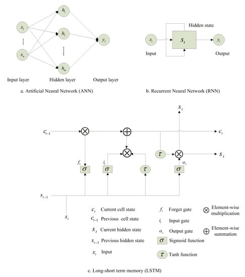
Figure 1.
The schematic architecture: (a) Artificial neural network (ANN), (b) Recurrent neural network (RNN), (c) Long short-term memory (LSTM).
2.2. Recurrent Neural Network (RNN)
Recurrent neural networks (RNNs) are an ANN where the past step outputs are supplied to the present phase as input. The unique of RNN is the feedback connection, which transmits information at the previous input that will be adjusted to the next input. RNN also has a hidden state vector or memory, which recalls some sequence data, and compute new states by employing its activation functions to prior states and new inputs recursively (see Figure 1b). This allows RNN to handle information sequentially and display temporal behavior for a time series while maintaining information from previous data. For RNNs, the hidden state vector in Equation (2) can be modified as in Equation (4):
where, is the matrix of weight parameter for the prior hidden state. RNNs can store memory as their present output depends on the preceding calculations. However, owing to the vanishing gradient issue, RNNs are known to go back only a few time steps, so the gradients that propagate back to the hidden units decrease exponentially when they are small.
2.3. Long Short-Term Memory (LSTM)
Hochreiter [28] suggested LSTM fixes the vanishing gradient issue in RNN intended to model temporal sequences. LSTM has long-range dependencies making LSTM more prices than standard RNNs. Unlike RNN, in the recurring hidden layer, LSTM includes unique units called memory cells. In the initial architecture, each memory cell contains three kinds of gates; input gate (regulating the flow into the memory cell of input activations), output gate (regulating the yield flow to the rest of the network of cell activations), and forget gate (scaling the cell’s inner state before adding it to the cell as input through the cell’s self-recurring association, thus forgetting or resetting the cell’s memory adaptively). The memory cell is the key to the LSTM framework. It goes directly down the entire chain with the capacity to add or extract cell state information, tightly controlled by structures called gates. The gates are optional data inlet ways. They consist of a neural net layer sigmoid and a point-sensitive multiplication as shown in Figure 1c. An input at time step and the hidden state of the preceding step brought to the LSTM cell, and then the hidden state is calculated as follows:
In LSTM, the first stage is to decide what data will be discarded from the cell state. The forget gate () (see Equation (5)) makes this choice:
where, is sigmoid function.
The next step is to decide which new information will be stored in the state of the cell. There are two tasks in this phase as at first, the input gate (see Equation (6) chooses which values to update. Secondly, a hyperbolic tangent (tanh) layer creates a vector of fresh values for the applicant values () as in Equation (7).
Then update the ancient state of the cell to the new state of the cell that can be provided as in Equation (8):
The output gate finally chooses which components of the cell state will be generated as output (see Equation (9)). The cell state then passes through the tanh layer and multiplies it as follows through the output gate as in Equation (10):
where: W and b are the matrix and bias of the weight parameter, respectively and is pointwise multiplication.
While the disappearing and exploding gradient issues in RNN were the results of inappropriate weights or gradient derivatives, the LSTM network did not suffer the same problems with its forget gate activation mechanism. LSTM allows networks to learn when to forget earlier hidden states and when to update hidden states with new data.
2.4. Genetic Algorithm (GA)
GA is a metaheuristic and stochastic algorithm inspired by the natural evolution process. They are commonly used in finding near-optimal solutions with big search spaces to optimize issues. GA has been widely applied to the neural network for time series forecasting. Azad et al. [29] employed GA for training ANN in order to predict minimum, mean, and maximum air temperature. GA can also be used to solve the optimization problem [30]. In another research, [31] applied the Scale Interaction Experiment Frontier research center for global change version 2 (SINTEX-F2) combined with GA to improve the air temperature prediction over various regions. The main characteristic of GA is the chromosomes, which have functions as a prospective solution to a target problem. These chromosomes are generated randomly and the one that offers the best result has more opportunity for reproduction. When operating from generation to generation, GA tends to seek better approximations to a problem solution. The following five steps summarize a straightforward operation of a GA:
- Generate an initial population of a collection of random chromosomes.
- Use the objective function to assess the fitness of chromosomes.
- Implement crossover and mutation to chromosomes according to their fitness.
- Generate a new population
- Repeats step ii–iv until the stopping requirements have been met.
We used the GA to select the best architecture and parameters for the neural network. In this study, we integrated neural network (NN) models including the deep-learning model (LSTM) and GA to find the customized number of epochs and hidden neurons for daily maximum temperature time series prediction.
3. Data Description
ANN, RNN, and LSTM models were applied to the time series of daily maximum temperature at the Cheongju station in South Korea; this station is located at 36.64° N, 127.44° E. We used the data for the period 1976–2015. For the target time series, we assumed that there was no long-term trend or cyclicity and that variable was normally distributed. In other words, we referred this assumption as the time series being stationary. To satisfy these conditions, the target time series had to be divided between the different seasons. Therefore, in this study, the data was divided into four seasons, namely winter (from December to February), spring (from March to May), summer (from June to August), and autumn (from September to November). Moreover, the stationarity of time series in four seasons was tested by the augmented Dickey–Fuller (ADF) test. The null hypothesis of the test is that the time series data is not stationary and the alternative hypothesis is that the time series is stationary [32]. Then, the dataset was standardized for each season as Equation (11):
where: and are the original and transformed explanatory variables, respectively and and are the mean and standard deviation of the original variable x, respectively.
Figure 2 showed a box plot for maximum temperature in four seasons over the period of study. In this figure, the orange line inside the boxes represented the median, and the upper and lower lines represented the 75th and 25th percentiles, respectively. The highest value of daily maximum temperature was observed in summer that being 38 °C, while the lowest was observed in winter that being −10 °C. The variability of maximum temperature in summer is smallest, followed by winter, autumn, and spring.
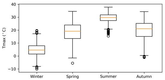
Figure 2.
Boxplot of the daily maximum temperature for every season.
4. Application Methodology
Our research relied closely on open source libraries under the Python environment [33]. Python is an interpreted, high-level programming language that can be used for a wide variety of applications, including research purposes. Our models were implemented using the Keras [34] toolkit, written in Python and TensorFlow [35], an open-source software library provided by Google. Additionally, other important packages such as NumPy [36], Pandas [37], and Matplotlib [38] were also used for processing, manipulating, and visualizing data.
In this section, we discussed the experimental methodology for the three state-of-the-art deep learning model, LSTM as well as ANN and RNN in detail. The dataset was divided into three sets as training, validation, and test sets. The training set was used to train the model, the validation set was used to evaluate the network’s generalization (i.e., overfitting), and the test set was used for network performance assessment. In the current study, 80% of the data (1976–2007) was selected as the training set, while the remaining 20% (2008–2015) was used as the test set. Furthermore, within the training set, a validation of 20% training set (2001–2007) was set aside to validate the performance of the model and preventing overfitting. In particular, the validation set was used for the hyperparameter optimization procedure, which is described later. We used the training set to fit models and made predictions corresponding to the validation set, then measured the root mean square error (RMSE) of those predicted values. Lastly, we determined the value of hyperparameters of the model by selecting the smallest RMSE on the validation set (optimum model) using the genetic algorithm (GA) as explained as follows:
We fit a training set with three different neural network models, namely ANN, RNN, and LSTM. Genetic parameters, such as crossover rate, mutation rate, and population size, can influence the outcome to obtain the optimal solution to the issue. In this research, we used in the experiment a population size of 10, 0.4 for crossover rate, and 0.1 for mutation rate [17]. A number of neurons in each hidden layer from 1 to 20, the number of epochs from 20 to 300, and the number of hidden layers from 1 to 3 will be evaluated. The tanh function is used as an activation function of the input and hidden neurons, while a linear function is designated as an activation function of output neurons in models. Initial weights of the network are set as random values, and a gradient-based “Adam” optimizer was used to adjust the network weights. GA solution would be decoded to get an integer number of epochs and a number of hidden neurons, which would then be used to train models. After that, RMSE on the validation set, which acts as a fitness function in this study, will be calculated. The solution with the highest fitness score was selected as the best solution. We implemented GA using distributed evolutionary algorithms in Python (DEAP) library [39]. Figure 3 illustrated the flowchart of the hybrid model proposed in our work.
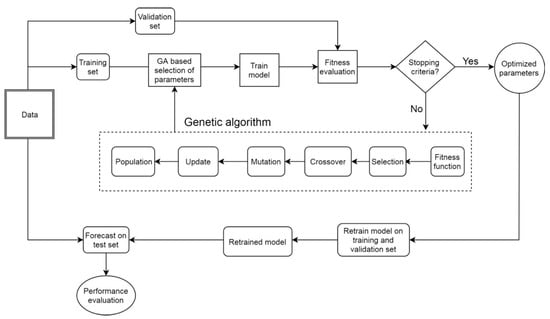
Figure 3.
Flowchart of the genetic algorithm and neural network model.
For each model, the dataset was trained with various cases of hidden layers, including one, two, and three hidden layers separately. The tanh function is used as an activation function of the input and hidden neurons while a linear function is designated as an activation function of output neurons in models. Initial weights of the network are set as random values, and a gradient-based “Adam” optimizer was used to adjust the network weights. GA solution would be decoded to get an integer number of epochs and number of hidden neurons, which would then be used to train models. After that, RMSE on the validation set, which acts as a fitness function in this study, will be calculated. The solution with the highest fitness score was selected as the best solution.
Genetic parameters, such as crossover rate, mutation rate, and population size, can influence the outcome to obtain the optimal solution to the issue. In this research, we used in the experiment a population size of 10, 0.4 for the crossover rate, and 0.1 for the mutation rate [15]. A number of neurons in each hidden layer from 1 to 20, the number of epochs from 20 to 300, and the number of hidden layers from 1 to 3 will be evaluated. The number of generations is allocated as 10 as a terminated condition [24]. We implemented GA using distributed evolutionary algorithms in Python (DEAP) library [28].
We fitted the model with optimal hyperparameters for both training and validation sets, and then used the test set for forecasting. Experiments were performed one- and multi-step-ahead prediction. At first, we forecasted one-day-ahead maximum temperature. Using the lag time technique, we split the time series into input and output. For modeling simplicity, in this study, past seven daily data values were employed to predict the daily maximum temperature for the next time (). To estimate the prediction accuracy and evaluate the performance of the forecast, three performance criteria, namely root mean square error (RMSE) (see Equation (12)), squared coefficient of correlation () (see Equation (13)), and mean absolute error (MAE) (see Equation (14)) were used; these can be calculated as follows:
where, is the current true value, is its predicted value, and n is the total number of testing data.
RMSE and MAE are commonly used to measure the difference between the predicted and observed values, while R2 indicates the fitness of the model to predict the maximum temperature. Furthermore, RMSE can be used to evaluate the closeness of these predictions to observations, while MAE can better represent prediction error. The ideal values of MAE and RMSE are definitely zero and R2 is certainly one, so the performance of a model obtains higher when the values of MAE and RMSE are close to zero and R2 is close to one. Each model (ANN, RNN, and LSTM) was fitted to the data for predicting one-day-ahead maximum temperature for the following three cases independently; using one-hidden-layer, two-hidden-layers, and three-hidden-layers.
Secondly, a multi-step ahead forecasting task was performed for predicting the next h values of a historical time series composed of m observations (lags). In order to obtain a multi-step-ahead prediction, we used the iteration technique [40], i.e., a prediction was used as input to obtain the prediction for the next time step. Finally, we had a sequence of predictions after h iteration steps. In the beginning, seven values were used as inputs for the first prediction. Moreover, it has been calculated that the more maximum temperature values were appended as inputs for the first prediction, the longer the predictions were produced more accurately. Thus, seven to thirty-six past temperature data (lags) were used as inputs for the first output. This work has been done for four seasons using ANN, RNN, and LSTM. In the current study, the best-defined architecture (number of epochs, number of hidden neurons, and number of hidden layers) for each of the distinct models (ANN, RNN, and LSTM) was selected to forecast 2-15-day-ahead maximum temperature in order to compare the efficiency of the different models for prediction with long lead times. The performance was measured by RMSE. Furthermore, as described above, we employed the different number of lags (7–36) for ANN, RNN, and LSTM models in each season to investigate the best number of lags based on the RMSE of 15-day-ahead prediction. The results from some trial runs revealed that increasing the number of lags beyond this level did not reduce the error for any of models considered, the experiment was stopped at 36 lags. The scatter plot of maximum temperature for four seasons was shown in Figure 4, which depicted the linear relationship between distinct lead times. As shown in Figure 4, most of the points in winter, spring, summer, and autumn followed a linear relationship. However, owing to some points with large variations from the linear relationship, it might be difficult for the models to learn the underlying pattern. Additionally, it can be observed that the association of the variable in summer in high values is higher than in low values for one-day-ahead, which can suspect that models might capture the pattern of high values better than low values. As the lead time increased, the patterns of data in winter and summer were considerably dispersed. Furthermore, the wide range of higher values in winter got wider at long lead times (k). In contrast, the lower values in spring, summer, and autumn expanded largely for longer range forecast.
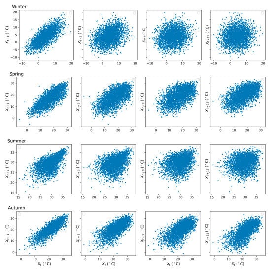
Figure 4.
Scatter plots of the observed daily maximum temperature and , in winter, spring, summer, and autumn.
5. Results
5.1. Data Stationarity Check
The confirmation of non-stationarity of four time series in winter, spring, summer, and autumn by an ADF test was provided in Table 1. From Table 1, we can see that the ADF statistic value of winter (−12.74450) was less than all critical values of −3.43221, −2.86236, and −2.56720 at 1%, 5%, and 10% respectively. Similarly, it is noticed that all ADF critical values in spring (−12.82992), summer (−12.11340), and autumn (−12.80105) were also smaller than critical values at 1%, 5%, and 10%. This suggested that the null hypothesis could be rejected with a significance level of less than 1%, 5%, and 10%. In another way, it indicated that all four time series in this study were stationary.

Table 1.
Augmented Dickey–Fuller test on maximum temperature data.
5.2. Model Performance
In this section, we described the qualitative and quantitative results for the different neural networks evaluated for maximum temperature prediction. It should be noted that the results listed in all the tables in this section indicate the efficiency of the respective model for the test data and not the training data since the training data had already been used in modeling and not much performance information can be given.
5.2.1. One-Day-Ahead Prediction
The best performance results for the ANN, RNN, and LSTM models used in this study for winter, spring, autumn, and summer are listed in Table 2, Table 3, Table 4 and Table 5, respectively. Each table presented the values of the hyperparameter in three cases of one, two, and three hidden layers that were optimally selected using the GA. From the results, it could be observed that summer had the lowest values for RMSE compared with winter, spring, and autumn. This can be attributed to the significantly smaller temperature variability in summer than in the other seasons, which was clear from Figure 3. In particular, the temperature range for summer was 20–38 °C, while those of winter, spring, and autumn were (−10)–18 °C, (−2)–35 °C, and 0–34 °C, respectively. Based on the values listed in Table 2, Table 3, Table 4 and Table 5, it is clear that the best results of ANN, RNN, and LSTM for every season were achieved using one-hidden-layer variant. In general, all three types of networks showed comparable performance, with small differences between the networks. The comparable performance explained that the models shown in those tables were trained and selected to their near-optimal values. Specifically, the results in Table 3 and Table 4 indicated that the best LSTM model performed better than the other models in terms of prediction in spring and summer. For spring, the optimal values of RMSE, MAE, and R2 were found to be as 3.59 °C, 2.92 °C, and 0.695, respectively using the LSTM model (see Table 3). The best values of statistics for summer were determined and given in Table 4. It can be seen from this table that the best RNN and LSTM model produced quite similar results for RMSE, MAE, and R2, which were 2.397 and 2.396, 1.901 and 1.909, 0.273 and 0.273, respectively. The lowest RMSE (2.404), MAE (1.904), and the highest R2 (0.269) of ANN, were also obtained using only one hidden layer. However, the ANN model showed a better result compared with LSTM and RNN in winter with the optimum values of RMSE, MAE, and R2 calculated as 2.981, 2.348, and 0.577, respectively (see Table 2).

Table 2.
The performance measure of models for winter.

Table 3.
The performance measure of models for spring.

Table 4.
The performance measure of models for summer.

Table 5.
The performance measure of models for autumn.
According to Table 5, the RNN model with one hidden layer presented the best performance for autumn with the values of 2.661, 2.093, and 0.840 for RMSE, MAE, and R2, individually. Figure 5, Figure 6, Figure 7 and Figure 8 showed the RMSE curves for varying number of hidden neurons in the three models with one hidden layer for the four seasons. The number of neurons in the hidden layer varied from 1 to 20 during the hidden neuron optimization step. For winter, the decrease rate of error (RMSE) with increasing the number of neurons in the hidden layer is shown in Figure 5. It can be observed that the performance of models (RNN and LSTM) was improved as the number of hidden neurons increased. The best numbers of RNN and LSTM units were derived as 11 and 10, respectively. However, for the ANN model, the rate of RMSE showed a considerable fluctuation when increasing the number of hidden neurons and the architecture with eight neurons in the hidden layer was chosen as the best ANN architecture. From Figure 6, it can be observed that the lowest MSE values of ANN, RNN, and LSTM in spring that were achieved during the neuron optimization were given by networks with 2, 5, and 3 hidden neurons, respectively. Similar to winter, the values of RMSE in summer for ANN showed a wide variation with the rising of neuron’s number and obtained the lowest value at two hidden neurons (see Figure 7). In addition, the lowest errors of RNN and LSTM were achieved with the number of hidden neurons of 8 and 3, respectively. In the case of autumn, we can notice from Figure 8 that the RMSE of LSTM reduced gradually when the number of neurons increased and achieved the minimum value at 14. Furthermore, Figure 8 illustrated that 6 and 3 hidden neurons produced ANN and RNN network with the lowest RMSE value, individually. From these figures, it can be observed that the LSTM model is more stable than the ANN and RNN models. Thus, it could be concluded that the output of ANN and RNN models was affected by the number of hidden neurons and was highly dependent on the hyperparameter selection.
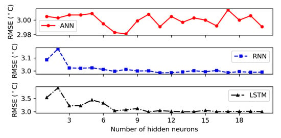
Figure 5.
Root mean square error corresponding to different number of hidden neurons for 1 hidden layer in winter.
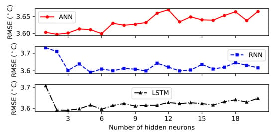
Figure 6.
Root mean square error corresponding to different number of hidden neurons for 1 hidden layer in spring.
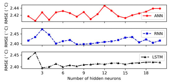
Figure 7.
Root mean square error corresponding to different number of hidden neurons for 1 hidden layer in summer.
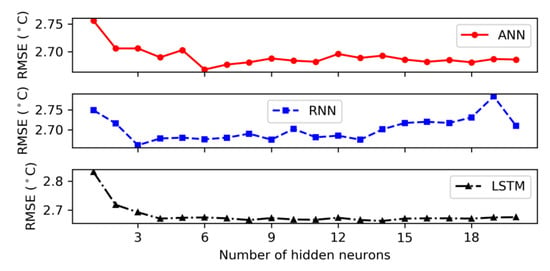
Figure 8.
Root mean square error corresponding to different number of hidden neurons for 1 hidden layer in autumn.
5.2.2. Multi-Day-Ahead Prediction
As discussed earlier, the best number of lags of each model (ANN, RNN, and LSTM) in four seasons was determined based on the performance of models on test set for 15 days prediction. The number of lags that return the smallest RMSE in 15-day-ahead forecast was selected as the best size of lags. Results are shown in Figure 9, where one can see the variation of RMSE for predicting the next 15 days in relation to the lags values (number of past maximum temperature measurements) used as inputs for the first output prediction. According to this figure, the best lags sizes of ANN, RNN, and LSTM in winter has been chosen as 19, 26, and 25, respectively. In spring, it was found that by using the temperature observed values of 33 days for ANN and RNN; and 34 days for LSTM, it is possible to predict daily temperatures for 15 days in advance with the smallest error. In addition, it is noted that in summer, ANN and RNN used 15 and 12 input data respectively while LSTM needed a larger number of lags (35) to predict with the smallest RMSE future maximum temperatures for 15 days. Finally, in autumn, the best size of lags for ANN was 25 meanwhile RNN and LSTM performed the best performance with the lags of 19. Table 6 lists the results for 1-15-day-ahead prediction for our models after choosing the best number of lags. Multi-day-ahead predictions in the table were made for the test set only. In all cases, 15-day-ahead forecasts have a greater error than one-day-ahead prediction for the same model; this is expected because of the accumulation of errors owing to the use of the iterative prediction procedure.
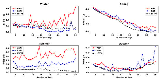
Figure 9.
Root mean square error corresponding to different number of lags of the next 15 days prediction.

Table 6.
Root mean square error (RMSE; °C) of test data of daily maximum temperature for predicting the next 15 days.
From the results listed in Table 6, it can be noted that in spring, and summer, the LSTM model had consistently better performance for long lead times compared with the other models. For summer, even though RNN had the best performance for one-day-ahead prediction, the LSTM model had the best results for long lead times ( days). Particularly, for 15-day-ahead temperature prediction, the RMSE of LSTM was 2.719 °C, while the RMSE of ANN was 3.014 °C and 2.822 °C or RNN. The RMSE value was decreased by about 9.8% and 3.6% compared to the error values of ANN and RNN models, respectively when using the LSTM model. For spring, the LSTM presented slightly better results than ANN and RNN for long term prediction in all lead times. Nevertheless, in winter and autumn, although RNN produced better results than ANN and LSTM for long term prediction, the error differences among three models were not significant. Furthermore, as mentioned above, in autumn, while LSTM showed better results for short lead times ( days), RNN generated the best performance for long term forecasting ( days) as prediction lead time increased. In winter, RNN produced lower RMSE than the others for overall lead times. Additionally, it can be noticed that the ANN model performed the worst result for all four seasons in the next 15 days prediction.
Figure 10 showed a comparison of the RMSE for the three models in all four seasons. Figure 10 indicated that the LSTM model is better performed than the ANN and RNN models for multi-day-ahead prediction in summer and spring. Moreover, it can be seen that the three lines in winter and autumn almost coincided indicating that ANN, RNN, and LSTM models have similar predictions. In summer, the RMSE of the LSTM model demonstrated significantly better results for long lead times (h) than the ANN and RNN models.
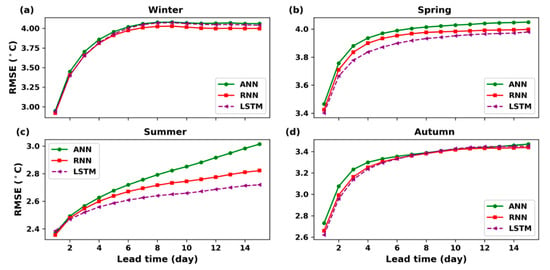
Figure 10.
RMSE of 15-day-ahead prediction for each season, (a) Winter, (b) Spring, (c) Summer, (d) Autumn.
The relation between the observed data and their predictions for multi-day-ahead forecasting in the four seasons for ANN, RNN, and LSTM models were illustrated in Figure 11, Figure 12, Figure 13 and Figure 14, respectively. From these figures, it can be noticed that the divergence between predicted and observed maximum temperature increased at longer prediction horizons. Moreover, the figures showed that most of low values were overestimated and high values were underestimated in case of long term prediction, especially in winter and summer (see Figure 11 and Figure 13). Figure 12 and Figure 14 depicted the scatter plot for maximum temperature predictions of the three models against the observed records in spring and autumn, respectively. It may be observed from these figures that the models predicted quite well for medium range of observed maximum temperature since the number of predicted day increased.
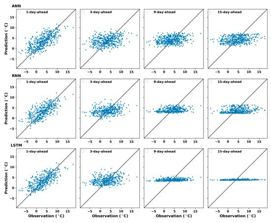
Figure 11.
Prediction of k days ahead using ANN (top), RNN (middle), and LSTM (bottom) models for winter, .
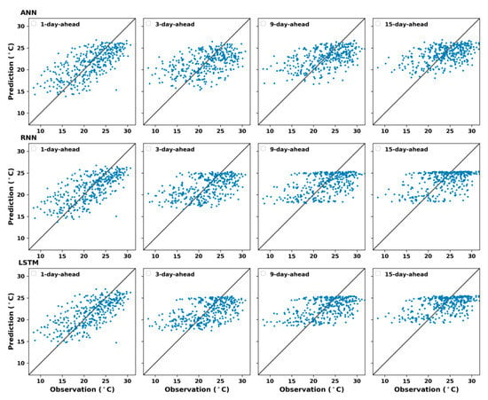
Figure 12.
Prediction of k days ahead using ANN (top), RNN (middle), and LSTM (bottom) models for spring, .
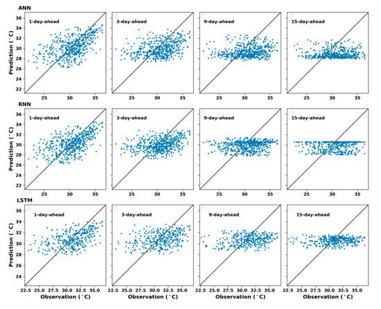
Figure 13.
Prediction of k days ahead using ANN (top), RNN (middle), and LSTM (bottom) models for summer, .
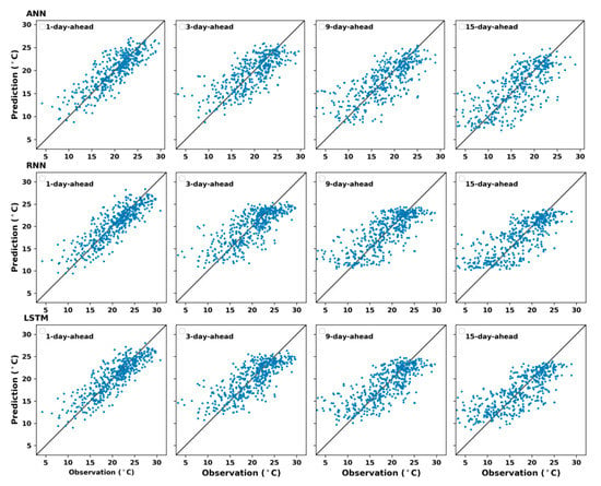
Figure 14.
Prediction of k days ahead using ANN (top), RNN (middle), and LSTM (bottom) models for autumn, .
6. Conclusions
In the current study, we applied the time series forecasting models of meteorological variables including the deep learning model (i.e., LSTM) assisted with the meta-learning for hyperparameter optimization. In particular, we forecasted the daily maximum temperature at the Cheongju station, South Korea up to 15 days in advance using the neural network models, ANN, and RNN as well as the deep-learning-based LSTM model. We integrated these models with GA to include the temporal properties of maximum temperature and utilized the customized architecture for the models.
GA was employed to obtain the optimal or near-optimal values of the number of epochs and the number of hidden units in neural network models through a meta-learning algorithm. Our results indicated that the LSTM model performed fairly well for long time scales in summer and spring than the other tested models in the current study. This can be attributed to the ability of LSTM models to maintain long-term memories, enabling them to process long sequences. In summary, the overall results demonstrated that the LSTM-GA approach efficiently maximum temperature in a season taking into consideration its temporal patterns.
This study shows that selecting the appropriate neural network architecture was important because it affected the temporal pattern and trend forecasting. To the best of our knowledge, in much of the existing literature, wherein neural networks were used to solve in time series problems, trial-and-error based methods rather than systematic approaches were used to obtain optimal hyperparameter values. However, we solved this issue by adopting GA, named as meta-learning. Our empirical results indicate the effectiveness of our proposed approach. Furthermore, the prediction that we made for the maximum temperature could be extended to other variables, including precipitation and wind speed. Thus, the method adopted in this study could be useful in determining the weather trend over a long-time period in a specific area.
Author Contributions
Conceptualization, formal analysis, T.T.K.T. and M.K.; Conceptualization, Resources, Methodology, Writing—original draft, T.L.; Conceptualization, Writing—original draft, Writing—review and editing, J.-S.K. and J.-Y.S. All authors have read and agreed to the published version of the manuscript.
Funding
This work was supported by the National Research Foundation of Korea (NRF) grant funded by the Korean Government (MEST) (2018R1A2B6001799).
Conflicts of Interest
The authors declare no conflict of interest.
References
- Sekula, P.; Bokwa, A.; Bochenek, B.; Zimnoch, M. Prediction of air temperature in the Polish Western Carpathian Mountains with the ALADIN-HIRLAM numerical weather prediction system. Atmosphere 2019, 10, 186. [Google Scholar] [CrossRef]
- Frnda, J.; Durica, M.; Nedoma, J.; Zabka, S.; Martinek, R.; Kostelansky, M. A weather forecast model accuracy analysis and ecmwf enhancement proposal by neural network. Sensors 2019, 19, 5144. [Google Scholar] [CrossRef] [PubMed]
- Fahimi Nezhad, E.; Fallah Ghalhari, G.; Bayatani, F. Forecasting Maximum Seasonal Temperature Using Artificial Neural Networks “Tehran Case Study”. Asia Pac. J. Atmos. Sci. 2019, 55, 145–153. [Google Scholar] [CrossRef]
- Nayak, D.R.; Mahapatra, A.; Mishra, P. A Survey on Rainfall Prediction using Artificial Neural Network. Int. J. Comput. Appl. 2013, 72, 32–40. [Google Scholar]
- Hassan, Z.; Shamsudin, S.; Harun, S.; Malek, M.A.; Hamidon, N. Suitability of ANN applied as a hydrological model coupled with statistical downscaling model: A case study in the northern area of Peninsular Malaysia. Environ. Earth Sci. 2015, 74, 463–477. [Google Scholar] [CrossRef]
- Liu, J.N.K.; Hu, Y.; You, J.J.; Chan, P.W. Deep neural network based feature representation for weather forecasting. In Proceedings of the International Conference on Artificial Intelligence (ICAI), Las Vegas, NV, USA, 21–24 July 2014. [Google Scholar]
- Schoof, J.T.; Pryor, S.C. Geography and Environmental Resources Downscaling Temperature and Precipitation: A Comparison of Regression-Based Methods and Artificial Neural Networks Comparison of Regresssion-Based Methods and Artificial. Int. J. Climatol. 2001, 21, 773–790. [Google Scholar] [CrossRef]
- Cao, Q.; Ewing, B.T.; Thompson, M.A. Forecasting wind speed with recurrent neural networks. Eur. J. Oper. Res. 2012, 221, 148–154. [Google Scholar] [CrossRef]
- Torres, J.L.; García, A.; De Blas, M.; De Francisco, A. Forecast of hourly average wind speed with ARMA models in Navarre (Spain). Sol. Energy 2005, 79, 65–77. [Google Scholar] [CrossRef]
- Agrawal, K. Modelling and prediction of rainfall using artificial neural network and ARIMA techniques. J. Ind. Geophys. Union 2006, 10, 141–151. [Google Scholar]
- Ustaoglu, B.; Cigizoglu, H.K.; Karaca, M. Forecast of daily mean, maximum and minimum temperature time series by three artificial neural network methods. Meteorol. Appl. 2008, 15, 431–445. [Google Scholar] [CrossRef]
- Altunkaynak, A. Forecasting surface water level fluctuations of lake van by artificial neural networks. Water Resour. Manag. 2007, 21, 399–408. [Google Scholar] [CrossRef]
- Chen, Y.; Chang, F. Evolutionary artificial neural networks for hydrological systems forecasting. J. Hydrol. 2009, 367, 125–137. [Google Scholar] [CrossRef]
- Tsai, Y.T.; Zeng, Y.R.; Chang, Y.S. Air pollution forecasting using rnn with lstm. In Proceedings of the 2018 IEEE 16th International Conference on Dependable, Autonomic and Secure Computing, Athens, Greece, 12–15 August 2018; pp. 1068–1073. [Google Scholar]
- Zhang, Q.; Wang, H.; Dong, J.; Zhong, G.; Sun, X. Prediction of Sea Surface Temperature Using Long Short-Term Memory. IEEE Geosci. Remote Sens. Lett. 2017, 14, 1745–1749. [Google Scholar] [CrossRef]
- Salman, A.G.; Heryadi, Y.; Abdurahman, E.; Suparta, W. Single Layer & Multi-layer Long Short-Term Memory (LSTM) Model with Intermediate Variables for Weather Forecasting. Procedia Comput. Sci. 2018, 135, 89–98. [Google Scholar] [CrossRef]
- Sagheer, A.; Kotb, M. Time series forecasting of petroleum production using deep LSTM recurrent networks. Neurocomputing 2019, 323, 203–213. [Google Scholar] [CrossRef]
- Hung, N.Q.; Babel, M.S.; Weesakul, S.; Tripathi, N.K. Hydrology and Earth System Sciences An artificial neural network model for rainfall forecasting in Bangkok, Thailand. Hydrol. Earth Syst. Sci. 2009, 13, 1413–1416. [Google Scholar] [CrossRef]
- Li, G.; Shi, J. On comparing three artificial neural networks for wind speed forecasting. Appl. Energy 2010, 87, 2313–2320. [Google Scholar] [CrossRef]
- Smith, B.A.; Mcclendon, R.W.; Hoogenboom, G. Improving Air Temperature Prediction with Artificial Neural Networks. Int. J. Comput. Inf. Eng. 2007, 3, 179–186. [Google Scholar]
- Zhang, G.; Patuwo, B.E.; Hu, M.Y. Forecasting with artificial neural networks: The state of the art. Int. J. Forecast. 1998, 14, 35–62. [Google Scholar] [CrossRef]
- Qi, M.; Zhang, G.P. An investigation of model selection criteria for neural network time series forecasting. Eur. J. Oper. Res. 2001, 132, 666–680. [Google Scholar] [CrossRef]
- Lemke, C.; Gabrys, B. Meta-learning for time series forecasting and forecast combination. Neurocomputing 2010, 73, 2006–2016. [Google Scholar] [CrossRef]
- Kordík, P.; Koutník, J.; Drchal, J.; Kovářík, O.; Čepek, M.; Šnorek, M. Meta-learning approach to neural network optimization. Neural Netw. 2010, 23, 568–582. [Google Scholar] [CrossRef] [PubMed]
- Bouktif, S.; Fiaz, A.; Ouni, A.; Serhani, M.A. Optimal deep learning LSTM model for electric load forecasting using feature selection and genetic algorithm: Comparison with machine learning approaches. Energies 2018, 11, 1636. [Google Scholar] [CrossRef]
- Chung, H.; Shin, K.S. Genetic algorithm-optimized long short-term memory network for stock market prediction. Sustainability 2018, 10, 3765. [Google Scholar] [CrossRef]
- Kolhe, M.; Lin, T.C.; Maunuksela, J. GA-ANN for short-term wind energy prediction. In Proceedings of the Asia-Pacific Power and Energy Engineering Conference, wuhan, China, 25–28 March 2011. [Google Scholar] [CrossRef]
- Hochreiter, S. Long Short-Term Memory. Neural Comput. 1997, 1780, 1735–1780. [Google Scholar] [CrossRef] [PubMed]
- Azad, A.; Pirayesh, J.; Farzin, S.; Malekani, L.; Moradinasab, S.; Kisi, O. Application of heuristic algorithms in improving performance of soft computing models for prediction of min, mean and max air temperatures. Eng. J. 2019, 23, 83–98. [Google Scholar] [CrossRef]
- Ahn, J.; Lee, J. Journal of geophysical research. Nature 1955, 175, 238. [Google Scholar]
- Ratnam, J.V.; Dijkstra, H.A.; Doi, T.; Morioka, Y.; Nonaka, M.; Behera, S.K. Improving seasonal forecasts of air temperature using a genetic algorithm. Sci. Rep. 2019, 9, 1–11. [Google Scholar] [CrossRef]
- Anokye, M.; Kwame, A.; Munyakazi, L. Modeling and Forecasting Rainfall Pattern in Ghana as a Seasonal Arima Process: The Case of Ashanti Region. Int. J. Humanit. Soc. Sci. 2013, 3, 224–233. [Google Scholar]
- Van Rossum, G. Python Tutorial; CWI (Centre for Mathematics and Computer Science): Amsterdam, The Netherlands, 1995. [Google Scholar]
- Chollet, F. Keras Documentation. Available online: https://keras.io/ (accessed on 4 May 2020).
- Abadi, M.; Agarwal, A.; Barham, P.; Brevdo, E.; Chen, Z.; Citro, C.; Corrado, G.S.; Davis, A.; Dean, J.; Devin, M.; et al. TensorFlow: Large-Scale Machine Learning on Heterogeneous Distributed Systems. arXiv 2016, arXiv:1603.04467. [Google Scholar]
- Van Der Walt, S.; Colbert, S.C.; Varoquaux, G. The NumPy array: A structure for efficient numerical computation. Comput. Sci. Eng. 2011, 13, 22–30. [Google Scholar] [CrossRef]
- McKinney, W. Data Structures for Statistical Computing in Python. In Proceedings of the 9th Python in Science Conference, Austin, TX, USA, 28 June–3 July 2010; pp. 51–56. [Google Scholar]
- Hunter, J.D. Matplotlib: A 2D graphics environment. Comput. Sci. Eng. 2007, 9, 99–104. [Google Scholar] [CrossRef]
- Fortin, F.-A.; De Rainville, F.-M.; Gardner, M.-A.; Parizeau, M.; Gagné, C. DEAP: Evolutionary Algorithms Made Easy François-Michel De Rainville. J. Mach. Learn. Res. 2012, 13, 2171–2175. [Google Scholar]
- Mihalakakou, G.; Santamouris, M.; Asimakopoulos, D. Modeling ambient air temperature time series using neural networks. J. Geophys. Res. Atmos. 1998, 103, 19509–19517. [Google Scholar] [CrossRef]
© 2020 by the authors. Licensee MDPI, Basel, Switzerland. This article is an open access article distributed under the terms and conditions of the Creative Commons Attribution (CC BY) license (http://creativecommons.org/licenses/by/4.0/).