Exploring Effective Chemical Indicators for Petrochemical Emissions with Network Measurements Coupled with Model Simulations

Abstract

A large petrochemical complex, dubbed Petro–complex, situated in a rather rural region of Taiwan, was used as a test bed to detect emissions from the Petro–complex to its surroundings. Hourly observations of speciated non–methane hydrocarbons (NMHCs) by the photochemical assessment monitoring stations (PAMSs), as well as the total amounts of NMHCs, SO₂, and NO_x provided by the air quality stations (AQSs), were utilized to find useful petro–emission indication methods. The analytical aspect of NMHCs either as a speciated form or as total amounts was demonstrated through field comparison to illustrate data quality. Using ethyne to offset traffic influence, the ratios of ethene to ethyne (acetylene) (E/A) and propene to ethyne (P/A) were proven to be effective indicators of petro–emissions owing to pronounced emissions of ethene and propene, revealed as tall spikes in PAMS measurements. SO₂ and NO_x were also explored as petro–emission indicators mainly for stack sources. By coordinating with three–dimensional modeling, SO₂ from petro–emissions could be distinguished from other prominent sources, such as coal–fired power plants. An attempt was also made to use SO₂ and NO_x as indicators of broader petro–emissions with stringent criteria to minimize traffic interference and increase specificity. Similar findings were observed with the three indicators, that is, volatile organic compounds (VOCs) ratios, SO₂ and NO_x, to identify the southwest area of the Petro–region as the most affected area, as represented by Taisi station (F2). The percent affected time of a year at F2 was 10%–14%, owing to the dominant wind field of northeast monsoonal (NEM) in the region, as compared with other sites in the east and north of 1–5%. Using VOC ratios as petro–emission indicators is more effective than using other gases, owing to the compositional advantage to minimize traffic interference.

1. Introduction

The petrochemical industry contributes significantly to the global economy. However, air pollutants from petrochemical facilities, such as volatile organic compounds (VOCs), particulate matter, SO₂, NO_x, heavy metals, polycyclic aromatic hydrocarbons (PAHs), and so on, have been frequently reported, some of which have been recognized as environmentally hazardous [1,2,3,4,5]. VOCs of stationary sources are mainly emitted from flaring, feedstock storage and distribution, solvent/reagent usage, as well as other chemical processes [6,7,8]. For a region with a major petrochemical facility, fugitive emissions, flaring, and stack emissions could be the major sources of VOCs dominating the ambient levels [9,10,11]. Studies have shown that VOC levels near a petrochemical facility could be much higher by a factor of 2–20 than in normal residential or suburban areas [6,7]. Although collectively, VOCs are precursors to ozone [12,13,14,15,16] and secondary organic aerosol (SOA) formation [16,17,18,19], some species such as chlorinated and aromatic compounds are also known to be toxic, and thus their prominent abundance in the air would be alarming to the public [20,21,22,23,24,25,26].

Sulfur dioxide, SO₂, has been a widely known air pollutant since the industrial revolution [27,28,29]. Its presence in the atmosphere is tightly associated with combustion of fossil fuel and it is released from stacks of power plants, petroleum refineries, smelters, and chemical plants [28,30]. For instance, sulfur dioxide from car emissions accounts for 0.13% of the total SO₂ budget, whereas the stack emissions account for 75.90% in Taiwan [31]. Anthropogenic SO₂ from non–stack fugitive emissions in industries was rarely observed [32]. Moreover, as a prominent air pollutant of the petrochemical industry and of high health relevance, SO₂ has been frequently studied [20,21,22]. Thus, identifying emission sources of VOCs, SO₂, and NO_x, particularly in industrial regions, is vital from the perspectives of public health and air quality.

Using observation–based approaches to identify prominent sources without resorting to complex statistical models, for example, chemical mass balance (CMB), principle component analysis (PCA), and positive matrix factorization (PMF), can sometimes be more straightforward and effective, provided that distinct source indicators or markers can be easily found [33]. For this purpose, selected compounds of VOCs are often used either as markers by the prominent presence in the air, or as ratios of certain compounds to offset air mixing and dilution. For instance, the presence of methyl tertiary butyl either (MTBE) in ambient air is tightly associated with on–road traffic [34]. A more elaborate approach is to use ratios of selected compounds that are co–sourced with methyl tert-butyl ether (MTBE) to cancel off effects of mixing and dilution [35]. Very often, the ratio of toluene to benzene within a range of 1~3 is deemed an indication of traffic source, whereas if the ratio goes beyond 3, it could be industrial in origin [7,36].

In this study, the “Petro–complex” is the largest petrochemical industrial complex on the island of Taiwan. To safe–guard air quality and public health in the region, nine air quality stations (AQSs) and photochemical assessment monitoring stations (PAMSs) were established near the complex to form a very densely deployed monitoring network closely watching emissions from the Petro–complex. The AQSs collected hourly data of SO₂, NO_x, CO, O₃, and Particulate Matter smaller than 10 μm (PM₁₀) and the total level of non–methane hydrocarbons (TNMHC). As TNMHC measurements do not provide speciated data of NMHCs, the PAMS sites were placed next to the AQS stations to report hourly mixing ratios of individual NMHCs. In our previous studies, a full year’s data from the nine stations were analyzed to recognize air pollutants transport routes from the Petro–complex under three major wind patterns covering 82% of the annual wind flows [37]. Moreover, source apportionment with validation and the impact from the Petro–complex on the surrounding areas has been successfully quantified by the method of positive matrix factorization (PMF) [38]. However, the data quality of PAMS and the exploration of key species of PAMS and AQS as effective emission indicator of the Petro–complex have not been discussed in depth. As a result, in this study, the establishment and data quality of PAMS are presented, followed by the source–receptor investigation using selected species of PAMS and AQS around the large Petro–complex as indicators of petro–emissions. The source investigation stresses heavily the hourly resolved observations coupled with model simulations to establish a distinct source–receptor relationship, which is highly wind directional. The methodology and findings resulting from this study could be applicable to any other prominent VOC emitters to facilitate source investigation.

2. Methods

2.1. Monitoring Facilities

The Formosa Petrochemical corporation is the sixth largest chemical company in the world [39], and the Petro–complex in this study is recognized as the most prominent VOC emitter in central coastal Taiwan as a stationary source. The Petro–complex occupies an area of 7.5 km × 4.5 km (2255 hectares). An extension eastwards to 20 km in radius from the Petro–complex forms the study domain, called the Petro–region. Nine AQSs and PAMSs were deployed within a 20 km radius of the coastal industrial complex in an area of approximately 18 × 25 km², with the distance between neighboring stations ranging from 5 to 10 km. All PAMSs were placed next to AQSs (AQS–F2 and AQS–F5 are hundreds of meters away from PAMS), as shown in Figure 1. Site F1, located on the roof of a six–floor building at the southern end of the industrial complex, served as the source monitoring station. The other eight sites (F2 to F9) were set up away from town centers and traffic arteries, and were thus considered as semi–rural sites.

The AQS network began monitoring hourly mixing ratios (or concentrations) of NO_x, NO, SO₂, CO, PM₁₀, O₃, as well as the total level of NMHCs (called AQS–TNMHC hereafter), from February 2013 to the present. The working theory of AQS–TNMHC is based on a subtractive method. The TNMHC concentration in an air sample aliquot is obtained from subtracting methane concentration from the total hydrocarbons (THCs). No separation of NMHC is needed. Usually, one measurement of TNMHC can be completed within minutes. Thus, minutely data can be averaged to become hourly data. The monitoring instruments at the nine AQS conformed to the specifications of the Taiwan Environmental Protection Administration (Taiwan EPA, see Supplementary Materials Table S1). Hourly measurements of 54 VOCs at the nine PAMS also began in October 2013. The working theory for PAMS measurements is based on gas chromatography (GC) to separate individual NMHCs of C₂ to C₁₂ with GC capillary columns. In our PAMS measurements, the separation needs an hour to complete, and thus the PAMS data are in hourly resolution. Both AQS–TNMHC and PAMS measurements involve the same detection principle, that is, flame ionization detection (FID). As FID basically works as a carbon counter, less complication can be anticipated when inter–compared between the two datasets.

Quality assurance and quality control (QC/QA) of PAMS observations were performed on a per–month basis. With the exclusion of routine maintenance, rare malfunctions, and QA injections of standard gas, data completeness was higher than 85% on average for all stations throughout the year [33].

The data length in this study is from October 2013 to September 2015. Hourly measurements for wind field, SO₂, NO_x, and AQS–TNMHC mixing ratios were obtained from the AQS network, whereas the 54 individual hourly NMHC mixing ratios were obtained from the PAMS network. Summation of the 54 NMHCs, dubbed PAMS–TNMHC, can be compared with AQS–TNMHC for mutual validation. When calculating PAMS–TNMHC, the true mixing ratios of all target compounds in parts per billion by volume (ppbv) are multiplied by their own carbon numbers to become methane–based mixing ratios (ppbC), which are then summed together to become the value of TNMHC. For AQS–TNMHC, the FID response of TNMHC as a single response is calibrated by a methane standard to be the value of AQS–TNMHC. As a result, both types of measurements are methane based and thus can be directly compared.

2.2. Wind Characteristics in the Petro–Region

In the Petro–region of this study, the wind field is highly seasonal and greatly affecting the transport routes of air pollutants. In order to systematically define air pollution characteristics from the Petro–complex, three major wind flow patterns were identified according to variations in daily wind direction (WD), that is, northeast monsoonal (NEM) flow, southwest monsoonal (SWM) flow, and local circulation/diffusion (LCD) [37]. These three types of wind fields are very characteristic throughout the island of Taiwan, but vary in strength and duration from north to south. In the central region, where the study domain was located, the three wind patterns occurred 79% of the time for the two year period from October 2013 to September 2015, during which the NEM flows accounted for 274 days or 39% of the time, occurring mostly from late fall to early spring (October to February); whereas the SWM flows accounted for 70 days or 10%, occurring mostly in summer; and the LCD accounted for 209 days or 30% of the time, occurring mostly in warm seasons during the period. For the remaining days, the wind types were too vague (such as typhoon or ambiguous wind fields) to be clearly categorized, and hence were not included in the assessment. The methods of identifying petro–emissions versus non–petro emissions in the following discussion are tested under the three characteristic wind fields.

2.3. Model Setup

The Fifth–Generation Penn State/NCAR Mesoscale Model (MM5) and the Taiwan air quality model (TAQM) were used for meteorological and air quality simulations. The horizontal grid sizes for the nested domains are 81 × 81 km² (D1), 27 × 27 km² (D2), 9 × 9 km² (D3), and 3 × 3 km² (D4), as shown in Figure S1. There are a total of 15 non–uniform sigma levels in the vertical direction from the surface to approximately 13.5 km above the surface, with the lowest level having a thickness of approximately 20 m. The simulation setup has been described in earlier studies [40,41].

3. Results and Discussion

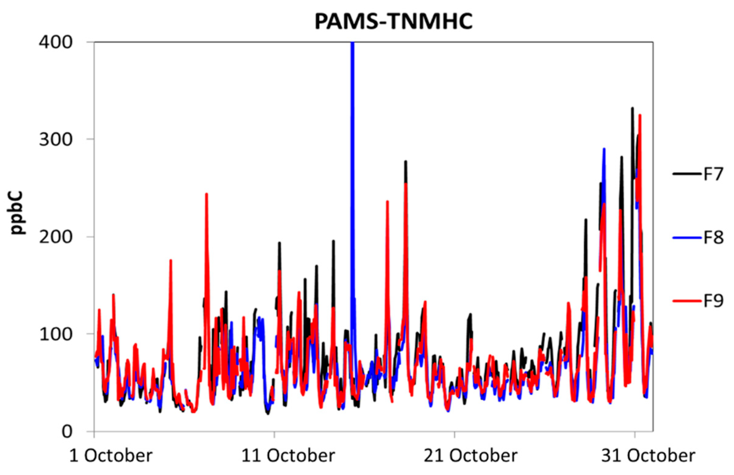
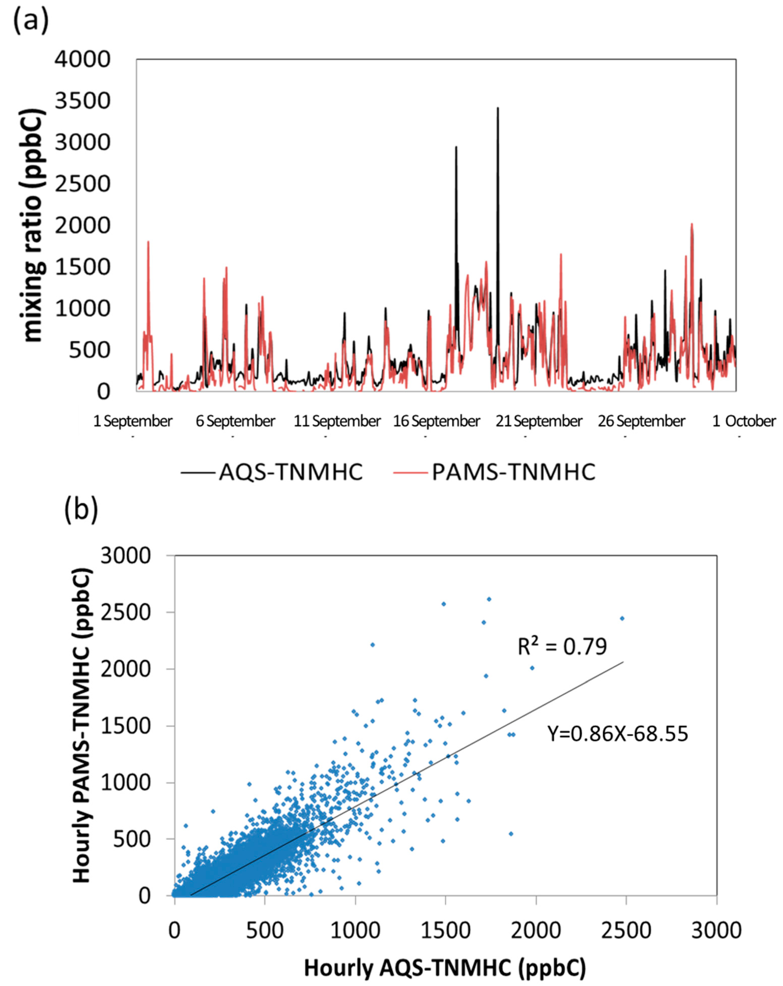
3.1. Validation of NMHC Observations

Despite separation by substantial distances in the Petro–region, occasionally, very coherent variations could be observed between PAMS sites under similar source influences and prevailing wind (Figure 2). We use this phenomenon to help validate the data quality of PAMS in addition to the routine quality assurance (QA) procedure. The high synchronicity in TNMHC between the three PAMS sites separated by 7–12 km from each other suggests the required quality in the PAMS’s calibration and measurements. Calibration and maintenance under one single protocol for all PAMS sites played a central role to ensure consistent data quality across all PAMS sites. Note that the synchronicity may not occur or disappear when these sites experienced different emission or meteorological influences. However, when the synchronicity does occur, it becomes very beneficial in terms of inspecting internal consistency and the overall data quality. For the two–year dataset, a number of relatively short periods of synchronicity occurred mostly under NEM when the wind field was sufficiently monotonous.

In general, PAMS–TNMHC measurements are highly correlated with AQS–TNMHC measurements, despite two different instruments [42]. We use site F1 as an illustration, which is located within the campus of Petro–complex, and is thus closest to the emissions. The two datasets, hourly mixing ratios of PAMS–TNMHC and AQS–TNMHC at site F1, were highly coherent with an R² = 0.79 (see Figure 3a,b). Note that, despite the high synchronicity of the two measurements, the PAMS–TNMHC values were consistently lower than the AQS–NMHC values by at least 20%, as can be observed by the much lower baseline of PAMS than of AQSs (Figure 3a), as well as the smaller than 1:1 ratio in the regression of the correlation plot in Figure 3b. The lower abundance of PAMS–TNMHC than of AQS–TNMHC can be rationalized in that only 54 NMHCs are targeted, whereas AQS–TNHC is responsive to all organics. For instance, oxygenated VOCs (denoted as OVOCs), such as alcohols, ketones, ethers, esters, and acids, produced and released in large amounts in the petrochemical industry, can be accounted for by AQS–TNMHC, but not by PAMS–TNMHC, despite a lower response than hydrocarbons. As a result, when it comes to reporting ambient VOC levels, AQS–TNMHC is a much better proxy than PAMS–TNMHC, because all organic compounds can be detected by FID, despite generally higher sensitivity for NMHC than for OVOCs [43,44]. Even though there is a shortfall of PAMS–TNMHC compared with AQS–TNMHC, the high coherence of the two, as shown in Figure 3a, suggests the 54 target NMHCs measured by PAMS played a dominant role in ambient VOC variabilities in the Petro–region.

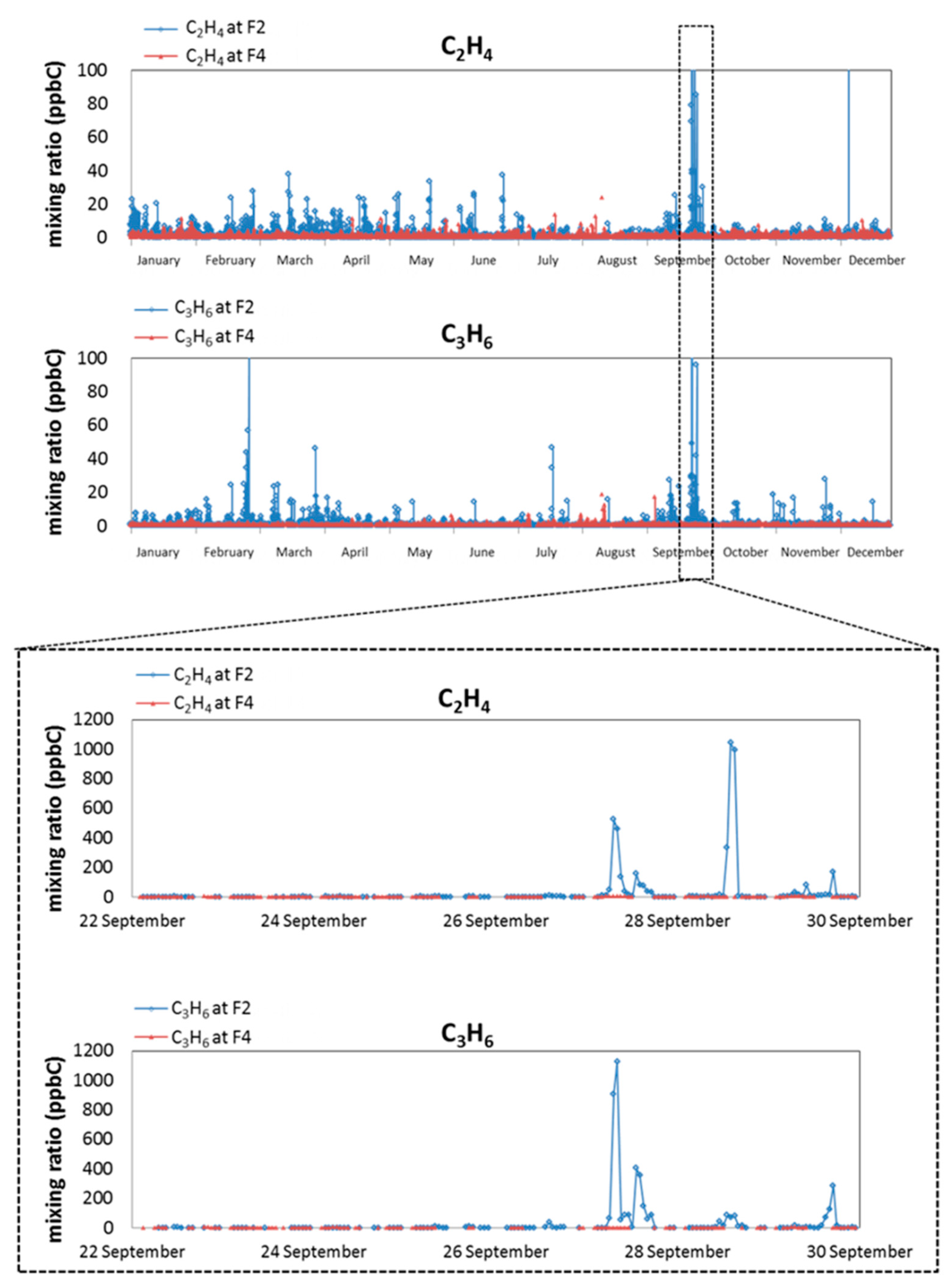
3.2. Ratios of P/A and E/A as Petro–Emission Indicators

It was found that ethene and propene were the two most pronounced compounds observed by PAMS, possibly owing to the extremely high volatility and the large quantities produced as feedstock of downstream plastic manufacture. Air masses coming from the Petro–complex are likely to be laden with these two very gaseous species. Although these two species do have a traffic source, the amounts were far less than the typical levels observed by the downwind PAMS sites. Concentrations of ethene and propene at F2 appeared as distinct spikes, as illustrated in Figure 4. Comparing F2 with F4, which are at the opposite directions of the Petro–complex on the northeast axis (see Figure 1), more spikes were encountered at F2 than at F4 owing to the dominant wind field of NEM in the region (upper two panels in Figure 4). These spike were often brief in time, for example, within a few hours, to suggest that the emissions coming off the Petro–complex were very direction sensitive. It appears that when the wind direction was in alignment with F2, ethene and propene as high as several hundred ppbv could be detected. The mixing ratios fell off rapidly and when the wind direction shifted even slightly to miss the monitoring site. As the area surrounding F2 is extremely rural, mixing ratios of ethene and propene were very close to the detection limits of the PAMS instrument. As a result, the sharp contrast between the sharp spikes and the low baseline was exploited as a form of indication of petro–emissions.

To exclude the traffic influence, a reference compound, ethyne (acetylene), which has no petro–sources and is mostly from car exhaust, is used as the common denominator in the ratios of ethene/ethyne (E/A) and propene/ethyne (P/A) to cancel off traffic contribution, as well as variability owing to air mixing. These three species can be obtained simultaneously from the PAMS network with hourly resolution. Thus, E/A and P/A were used as effective indicators of petro–emissions in the region, and the thresholds of E/A > 3 and P/A > 1.5 were set to differentiate air masses affected by the petro–emissions from those that are not affected [33]. The usefulness of the two ratio indicators is illustrated for the three characteristic seasonal wind fields as follows.

Under the NEM flow, which prevailed mostly in fall and winter, wind direction in the region was mainly between 315 and 45 degrees; hence, Site F2, in the southwest of the Petro–complex, would be more affected by the Petro–complex’s emissions than F4~F9, which are spread over from the north to the east of the Petro–complex and further inland. Under the SWM flow, which mostly prevailed in summer, wind direction was mostly between 135 and 225 degrees; hence, petro–emissions were more likely to affect site F4, situated at the north of the Petro–complex (see Figure 1 for site F4 location). Under the LCD flow, the affected downwind sites varied considerably owing to the rapidly changing wind direction, and the influences from the Petro–complex would be more towards the inland area than the coastal. Some typical cases are demonstrated in Figure 5. Under the NEM flow (Figure 5a), the simultaneous increase in PAMS–TNMHC mixing ratios as well as P/A and E/A ratios at site F2 indicated that this area was more affected by the petro–emissions during the evening hours. Although a concentration peak also appeared at F9, the lower–than–threshold in P/A and E/A values suggests that F9 was not affected by petro–emissions, but more likely by traffic sources. Under the SWM flow (Figure 5b), the wind field is nearly the opposite of NEM, and high PAMS–TNMHC mixing ratios appeared at night for all sites, but only at noon for site F4; however, the E/A and P/A ratios suggest that only site F4 was affected by petro–emissions at noon. Thus, F2 and F4 can be either the upwind or downwind site depending upon the seasonality and the prevailing wind field.

Under the LCD flow (Figure 5c), the PAMS–TNMHC mixing ratios varied dramatically within a time frame of only a few hours owing to the rapidly changing wind directions. The VOC–based ratios indicated that site F2 and F4 were highly influenced by the petro–emissions, whereas F9 was less affected mostly around noontime.

3.3. SO₂ and NO_x with Modeling to Indicate Stack Plumes

In addition to fugitive emissions and flaring, which can be detected by PAMS–derived indicators of E/A and P/A, flue gas released as plumes from stacks of the Petro–complex containing both VOCs as well as SO₂ and NO_x can be put to the test for the effectiveness as indicators. The idea is that SO₂ and NO_x in the plumes should be much higher in concentrations than outside the plumes. Although stack plumes from the petro–industry contain relatively high levels of SO₂ and NO_x, their specificity is generally low owing to the lack of compositional features. For instance, differentiation of plumes from the petro–industry from the plumes coming off the fire power plants can be difficult, as both types of sources contain high levels of the two pollutants. Unless plume detection by these two gases can be supported by other means, the specificity could be in question. As a supporting tool, air–quality modeling was used to enhance the petro–plume indication with SO₂ and NO_x. For demonstration, three characteristic wind fields of NEM, SWM, and LCD are exemplified as follows.

Despite the rather monotonous wind characteristics with the NEM flow, the source–receptor relationship can still be ambiguous at times. Figure 6 and Figure 7 illustrate an example of the wind direction affecting plume source identification. A large coal burning fire power plant (5824 mWatts), the second largest worldwide, located 60 km north of the Petro–region (as show in Figure 1), releases SO₂ and NO_x from stacks of 250 m height. At a very specific angle of the NEM flow, the smoke plumes from the power plant may merge with the plume tracks from the Petro–complex and become indistinguishable from the petro–plumes, and thus are often perceived as local petro–emissions. However, this misconception can be easily divulged by the combination of on–site measurements and modeling. Thus, hourly data of SO₂ and NO_x provided by AQS were examined for the plume influences on the Petro–region. Under the prevailed northeasterly wind, site F2, a downwind site of both the power plant and the Petro–complex, can receive the merged plumes or single plume form the Petro–complex. When the wind slightly shifted in direction, the merged plumes then diverged, and only F2, at the southwest of the Petro–complex, was affected by the Petro–complex’s stack emissions, as revealed by the elevated SO₂ level (black box in Figure 6 and Figure 7a). Moreover, site F4 is at the northeast of the Petro–region, and thus could not possibly be influenced by the Petro–complex under the prevailed northeasterly wind. Hence, the stack plumes elevated the SO₂ and NO_x concentrations at F4 at around 09:00, as indicated by the yellow box in Figure 6. Site F2, however, can receive the merged plumes. Figure 7b provides a complete pictorial view of the plume tracks from both sources under the particular wind flow. The slightly elevated SO₂ and NO_X levels at other sites to the east were mostly contributed by the power plant plumes. The divergence of the two plume tracks became even more obvious in the evening hours as the wind shifted from northeasterly to northerly. F9, the most inland and eastward site from the Petro–complex, was entirely affected by the power plant emissions and not by petro–plumes to show the highest levels of SO₂ and NO_X among all sites, as indicated by the red box in Figure 6 and the simulation in Figure 7c. As a result, using SO₂ and NO_x as plume indicators to investigate the source–receptor relationship can be obscure at times if not aided by other means such as modeling to provide a more realistic view (See Figure S2 for the comparison of simulations with observations on 10 October 2013).

Under the SWM flow, clean marine air was brought from the south to the Petro–region. All stations except F4 would show comparable and relatively low levels of pollutants owing to the influence from the clean marine air and greater mixing heights in warm seasons. However, site F4 would occasionally show elevated levels of SO₂ and NO_x when the petro–plumes arrives at the downwind site F4, as shown in Figure 8 for the observed concentration peaks (black box in Figure 8a) accompanied by simulation results (Figure 8b). Again, measurements and modeling combined are able to help investigate the source–receptor relationship with clarity (See Figure S3 for the comparison of simulations with observations on 19 June 2014).

Note that, although Figure 6, Figure 7, and Figure 8 only show brief periods of data, they are intended to illustrate typical features of the source–receptor relationship under the very repetitive and seasonal wind patterns. With the tools of modeling and densely deployed monitoring facilities, these features can be adequately characterized.

3.4. Test of SO₂ and NO_X as Petro–Emission Indicators

The PAMS derived ratios of E/A > 3 and P/A > 1.5 have proven to be effective petro–emission indicators. However, PAMS is usually not a typical establishment for air quality assessment worldwide. For general air quality indication, SO₂ and NO_x are more readily available as standardized methods adopted by environmental protection agencies. When assisted with model simulations, SO₂ and NO_x can be used as plume tracers, as illustrated earlier. However, when traffic source comes into play in more populated areas, the conditions of using SO₂ and NO₂ as petro–indicators have to be restricted by more stringent boundaries to be indicative enough of petro–emissions.

The attempt of using SO₂ and NO_x as petro–emission indicators was bound by the following three criteria. First, the Petro–complex has to be upwind of the given monitoring sites in the Petro–region under a given prevailing wind direction. Second, the SO₂ and NO_x data used for analysis are required to be significantly greater than the baseline values, that is, twice the standard deviations or higher. Note that the baseline values for the two gases were determined by the lowest 25% of the dataset. Third, SO₂ and NO_x should be free from prominent sources other than the Petro–complex, such as fire power plants, steel mills, and cement plants. For instance, if SO₂ and NO_x at both F2 and F4 exceeded the baseline criteria, then the downwind site (F2) was considered as polluted by other sources than the petro–emissions, and thus the data were excluded.

The percent time affected by Petro–complex emissions during 2014 and 2015 for the areas represented by F2, F4, and F9, representing south, north, and east, were calculated with the two years of hourly monitoring data based on the three different indicators of VOC ratios, SO₂, and NO_x. The percent time affected at F2 was 14.0%, 10.7%, and 9.7% for VOC ratios, SO₂, and NO_x, respectively; 1.8%, 3.4%, and 4.0% at F4, respectively; and 1.4%, 3.1%, and 5.1% at F9, respectively. Because the wind characteristics in the region are very seasonal and repetitive year after year, we believe the findings based on two years of hourly measurements are sufficiently representative of the region. It is evident that all three indicators were able to identify F2 as the most affected site by the Petro–complex, as it was in alignment with the Petro–complex under NEM, which is the dominant wind field in colder seasons with lower mixing heights and rather monotonous wind directions. In contrast, the other sites to the east (as represented by F9) or north (as represented by F4) were remarkably less affected by the Petro–complex. Although all three indicators resulted in similar findings of identifying F2 as the most affected site, the use of SO₂ and NO_x was subjected to many restrictions when to minimize traffic interference. Furthermore, the discrepancy between the three indicators for a given site could result from the incomplete removal of traffic interference despite strict reconditions set for SO₂ and NO_x. In this regard, VOC–based indicators can be more useful than other gases, as they can be extremely sensitive and better exempted from traffic interference owing to the compositional advantage.

4. Conclusions

A large Petro–complex in a rather rural area was exploited as a test ground for investigating petro–emission indicators. The extensively deployed PAMS and AQS sites in the region providing hourly data of speciated NMHCs, as well as SO₂ and NO_x, were utilized for indication of petro–emissions. Data quality of PAMS played a pivotal role in the data utilization, and thus was validated by comparison among PAMS sites and between AQS–TNMHC and PAMS–TNMHC to show internal consistency. The VOC ratios of E/A and P/A were found very useful as petro–emission indicators owing to the prominent emissions of ethene and propene from refinery. SO₂ can be used as an indicator for stack emissions if assisted with model simulations to decouple contribution from other prominent SO₂ sources such as distant fire power plants. When there is no PAMS available, SO₂ and NO_x can be used as emission indicators of the Petro–complex, provided that they are bound by stringent criteria to minimize traffic interference. Similar findings were observed with the three indicators of VOC ratios, SO₂, and NO_x to identify F2 as the most affected site owing to the dominant wind field of NEM in the region. The VOC–based indicators are more effective in tracing petro–emissions than other gases such as SO₂ or NO_x owing to the compositional advantage with the VOC data to minimize traffic interference.

References

1. Baltrėnas, P.; Baltrėnaitė, E.; Šerevičienė, V.; Pereira, P. Atmospheric BTEX concentrations in the vicinity of the crude oil refinery of the Baltic region. Environ. Monit. Assess. 2011, 182, 115–127. [Google Scholar] [CrossRef]
2. Nadal, M.; Schuhmacher, M.; Domingo, J.L. Long—Term environmental monitoring of persistent organic pollutants and metals in a chemical/petrochemical area: Human health risks. Environ. Pollut. 2011, 159, 1769–1777. [Google Scholar] [CrossRef]
3. Mo, Z.; Shao, M.; Lu, S.; Qu, H.; Zhou, M.; Sun, J.; Gou, B. Process–specific emission characteristics of volatile organic compounds (VOCs) from petrochemical facilities in the Yangtze River Delta, China. Sci. Total Environ. 2015, 533, 422–431. [Google Scholar] [CrossRef]
4. Kampeerawipakorn, O.; Navasumrit, P.; Settachan, D.; Promvijit, J.; Hunsonti, P.; Parnlob, V.; Nakngam, N.; Choonvisase, S.; Chotikapukana, P.; Chanchaeamsai, S.; et al. Health risk evaluation in a population exposed to chemical releases from a petrochemical complex in Thailand. Environ. Res. 2017, 152, 207–213. [Google Scholar] [CrossRef]
5. Hsu, C.-Y.; Chiang, H.-C.; Shie, R.-H.; Ku, C.-H.; Lin, T.-Y.; Chen, M.-J.; Chen, N.-T.; Chen, Y.-C. Ambient VOCs in residential areas near a large—Scale petrochemical complex: Spatiotemporal variation, source apportionment and health risk. Environ. Pollut. 2018, 240, 95–104. [Google Scholar] [CrossRef]
6. Cetin, E.; Odabasi, M.; Seyfioglu, R. Ambient volatile organic compound (VOC) concentrations around a petrochemical complex and a petroleum refinery. Sci. Total Environ. 2003, 312, 103–112. [Google Scholar] [CrossRef]
7. Tiwari, V.; Hanai, Y.; Masunaga, S. Ambient levels of volatile organic compounds in the vicinity of petrochemical industrial area of Yokohama, Japan. Air Qual. Atmos. Health 2010, 3, 65–75. [Google Scholar] [CrossRef] [Green Version]
8. Huang, Y.S.; Hsieh, C.C. Ambient volatile organic compound presence in the highly urbanized city: Source apportionment and emission position. Atmos. Environ. 2019, 206, 45–59. [Google Scholar] [CrossRef]
9. Zhang, Z.; Wang, H.; Chen, D.; Li, Q.; Thai, P.; Gong, D.; Li, Y.; Zhang, C.; Gu, Y.; Zhou, L.; et al. Emission characteristics of volatile organic compounds and their secondary organic aerosol formation potentials from a petroleum refinery in Pearl River Delta, China. Sci. Total Environ. 2017, 584–585, 1162–1174. [Google Scholar] [CrossRef] [Green Version]
10. Hu, B.; Xu, H.; Deng, J.; Yi, Z.; Chen, J.; Xu, L.; Hong, Z.; Chen, X.; Hong, Y. Characteristics and Source Apportionment of Volatile Organic Compounds for Different Functional Zones in a Coastal City of Southeast China. Aerosol Air Qual. Res. 2018, 18, 2840–2852. [Google Scholar] [CrossRef]
11. Gu, Y.; Li, Q.; Wei, D.; Gao, L.; Tan, L.; Su, G.; Liu, G.; Liu, W.; Li, C.; Wang, Q. Emission characteristics of 99 NMVOCs in different seasonal days and the relationship with air quality parameters in Beijing, China. Ecotoxicol. Environ. Saf. 2019, 169, 797–806. [Google Scholar] [CrossRef] [PubMed]
12. Carter, W.P.L. A detailed mechanism for the gas–phase atmospheric reactions of organic compounds. Atmos. Environ. Part A Gen. Top. 1990, 24, 481–518. [Google Scholar] [CrossRef]
13. Carter, W.P.L. Development of Ozone Reactivity Scales for Volatile Organic Compounds. Air Waste 1994, 44, 881–899. [Google Scholar] [CrossRef] [Green Version]
14. Seinfeld, J.H.; Pandis, S.N. Atmospheric Chemistry and Physics; Wiley: New York, NY, USA, 1998. [Google Scholar]
15. Atkinson, R.; Arey, J. Atmospheric Degradation of Volatile Organic Compounds. Chem. Rev. 2003, 103, 4605–4638. [Google Scholar] [CrossRef]
16. Hui, L.; Liu, X.; Tan, Q.; Feng, M.; An, J.; Qu, Y.; Zhang, Y.; Deng, Y.; Zhai, R.; Wang, Z. VOC characteristics, chemical reactivity and sources in urban Wuhan, central China. Atmos. Environ. 2020, 224, 117340. [Google Scholar] [CrossRef]
17. Huang, R.-J.; Zhang, Y.; Bozzetti, C.; Ho, K.-F.; Cao, J.-J.; Han, Y.; Daellenbach, K.R.; Slowik, J.G.; Platt, S.M.; Canonaco, F.; et al. High secondary aerosol contribution to particulate pollution during haze events in China. Nature 2014, 514, 218–222. [Google Scholar] [CrossRef] [Green Version]
18. Yao, L.; Garmash, O.; Bianchi, F.; Zheng, J.; Yan, C.; Kontkanen, J.; Junninen, H.; Mazon, S.B.; Ehn, M.; Paasonen, P.; et al. Atmospheric new particle formation from sulfuric acid and amines in a Chinese megacity. Science 2018, 361, 278–281. [Google Scholar] [CrossRef] [Green Version]
19. Xu, L.; Tsona, N.T.; You, B.; Zhang, Y.; Wang, S.; Yang, Z.; Xue, L.; Du, L. NOx enhances secondary organic aerosol formation from nighttime γ-terpinene ozonolysis. Atmos. Environ. 2020, 225, 117375. [Google Scholar] [CrossRef]
20. Chen, P.C.; Lai, Y.M.; Wang, J.D.; Yang, C.Y.; Hwang, J.S.; Kuo, H.W.; Huang, S.L.; Chan, C.C. Adverse effect of air pollution on respiratory health of primary school children in Taiwan. Environ. Health Perspect. 1998, 106, 331–335. [Google Scholar] [CrossRef]
21. Yang, C.-Y.; Wang, J.-D.; Chan, C.-C.; Hwang, J.-S.; Chen, P.-C. Respiratory symptoms of primary school children living in a petrochemical polluted area in Taiwan. Pediatric Pulmonol. 1998, 25, 299–303. [Google Scholar] [CrossRef]
22. Smargiassi, A.; Kosatsky, T.; Hicks, J.; Plante, C.; Armstrong, B.; Villeneuve Paul, J.; Goudreau, S. Risk of Asthmatic Episodes in Children Exposed to Sulfur Dioxide Stack Emissions from a Refinery Point Source in Montreal, Canada. Environ. Health Perspect. 2009, 117, 653–659. [Google Scholar] [CrossRef] [PubMed] [Green Version]
23. Huang, B.; Lei, C.; Wei, C.; Zeng, G. Chlorinated volatile organic compounds (Cl-VOCs) in environment—Sources, potential human health impacts, and current remediation technologies. Environ. Int. 2014, 71, 118–138. [Google Scholar] [CrossRef] [PubMed]
24. Huang, P.-C.; Liu, L.-H.; Shie, R.-H.; Tsai, C.-H.; Liang, W.-Y.; Wang, C.-W.; Tsai, C.-H.; Chiang, H.-C.; Chan, C.-C. Assessment of urinary thiodiglycolic acid exposure in school–aged children in the vicinity of a petrochemical complex in central Taiwan. Environ. Res. 2016, 150, 566–572. [Google Scholar] [CrossRef] [PubMed]
25. Yuan, T.-H.; Shen, Y.-C.; Shie, R.-H.; Hung, S.-H.; Chen, C.-F.; Chan, C.-C. Increased cancers among residents living in the neighborhood of a petrochemical complex: A 12–year retrospective cohort study. Int. J. Hyg. Environ. Health 2018, 221, 308–314. [Google Scholar] [CrossRef] [PubMed]
26. Yuan, T.-H.; Ke, D.-Y.; Wang, J.E.-H.; Chan, C.-C. Associations between renal functions and exposure of arsenic and polycyclic aromatic hydrocarbon in adults living near a petrochemical complex. Environ. Pollut. 2020, 256, 113457. [Google Scholar] [CrossRef] [PubMed]
27. Guttikunda, S.K.; Carmichael, G.R.; Calori, G.; Eck, C.; Woo, J.-H. The contribution of megacities to regional sulfur pollution in Asia. Atmos. Environ. 2003, 37, 11–22. [Google Scholar] [CrossRef]
28. Huang, J.-T. Sulfur dioxide (SO2) emissions and government spending on environmental protection in China – Evidence from spatial econometric analysis. J. Clean. Prod. 2018, 175, 431–441. [Google Scholar] [CrossRef]
29. Liu, F.; Choi, S.; Li, C.; Fioletov, V.E.; McLinden, C.A.; Joiner, J.; Krotkov, N.A.; Bian, H.; Janssens-Maenhout, G.; Darmenov, A.S.; et al. A new global anthropogenic SO2 emission inventory for the last decade: A mosaic of satellite-derived and bottom-up emissions. Atmos. Chem. Phys. 2018, 18, 16571–16586. [Google Scholar] [CrossRef] [Green Version]
30. Greenstone, M. Did the Clean Air Act cause the remarkable decline in sulfur dioxide concentrations? J. Environ. Econ. Manag. 2004, 47, 585–611. [Google Scholar] [CrossRef]
31. Taiwan Environmental Protection Agency. Taiwan Emission Data System. 2019. Available online: https://teds.epa.gov.tw/TEDS_10_10.aspx (accessed on 10 March 2020).
32. U.S Environmental Protection Agency. Sulfur Dioxide Emissions. 2020. Available online: https://cfpub.epa.gov/roe/indicator.cfm?i=22 (accessed on 10 March 2020).
33. Su, Y.-C.; Chen, S.-P.; Tong, Y.-H.; Fan, C.-L.; Chen, W.-H.; Wang, J.-L.; Chang, J.S. Assessment of regional influence from a petrochemical complex by modeling and fingerprint analysis of volatile organic compounds (VOCs). Atmos. Environ. 2016, 141, 394–407. [Google Scholar] [CrossRef]
34. Chang, C.-C.; Lo, S.-J.; Lo, J.-G.; Wang, J.-L. Analysis of methyl tert–butyl ether in the atmosphere and implications as an exclusive indicator of automobile exhaust. Atmos. Environ. 2003, 37, 4747–4755. [Google Scholar] [CrossRef]
35. Chang, C.-C.; Wang, J.-L.; Liu, S.-C.; Candice Lung, S.-C. Assessment of vehicular and non–vehicular contributions to hydrocarbons using exclusive vehicular indicators. Atmos. Environ. 2006, 40, 6349–6361. [Google Scholar] [CrossRef]
36. Shaw, M.D.; Lee, J.D.; Davison, B.; Vaughan, A.; Purvis, R.M.; Harvey, A.; Lewis, A.C.; Hewitt, C.N. Airborne determination of the temporo-spatial distribution of benzene, toluene, nitrogen oxides and ozone in the boundary layer across Greater London, UK. Atmos. Chem. Phys. 2015, 15, 5083–5097. [Google Scholar] [CrossRef] [Green Version]
37. Chen, S.-P.; Wang, C.-H.; Lin, W.-D.; Tong, Y.-H.; Chen, Y.-C.; Chiu, C.-J.; Chiang, H.-C.; Fan, C.-L.; Wang, J.-L.; Chang, J.S. Air quality impacted by local pollution sources and beyond—Using a prominent petro–industrial complex as a study case. Environ. Pollut. 2018, 236, 699–705. [Google Scholar] [CrossRef] [PubMed]
38. Su, Y.-C.; Chen, W.-H.; Fan, C.-L.; Tong, Y.-H.; Weng, T.-H.; Chen, S.-P.; Kuo, C.-P.; Wang, J.-L.; Chang, J.S. Source Apportionment of Volatile Organic Compounds (VOCs) by Positive Matrix Factorization (PMF) supported by Model Simulation and Source Markers—Using Petrochemical Emissions as a Showcase. Environ. Pollut. 2019, 254, 112848. [Google Scholar] [CrossRef]
39. Tullo, A.H. C&EN’s Global Top 50 chemical companies of 2018. Chem. Eng. News 2019, 97, 30. [Google Scholar]
40. Chen, S.-P.; Liu, T.-H.; Chen, T.-F.; Yang, C.-F.O.; Wang, J.-L.; Chang, J.S. Diagnostic Modeling of PAMS VOC Observation. Environ. Sci. Technol. 2010, 44, 4635–4644. [Google Scholar] [CrossRef]
41. Chiang, C.-K.; Fan, J.-F.; Li, J.; Chang, J.S. Impact of Asian continental outflow on the springtime ozone mixing ratio in northern Taiwan. J. Geophys. Res. Atmos. 2009, 114. [Google Scholar] [CrossRef] [Green Version]
42. Chen, S.-P.; Liao, W.-C.; Chang, C.-C.; Su, Y.-C.; Tong, Y.-H.; Chang, J.S.; Wang, J.-L. Network monitoring of speciated vs. total non-methane hydrocarbon measurements. Atmos. Environ. 2014, 90, 33–42. [Google Scholar] [CrossRef]
43. Dietz, W.A. Response Factors for Gas Chromatographic Analyses. J. Chromatogr. Sci. 1967, 5, 68–71. [Google Scholar] [CrossRef]
44. Scanlon, J.T.; Willis, D.E. Calculation of Flame Ionization Detector Relative Response Factors Using the Effective Carbon Number Concept. J. Chromatogr. Sci. 1985, 23, 333–340. [Google Scholar] [CrossRef]
Figure 1. Area within a 20 km radius of the Petro–complex is dubbed the Petro–region, as indicated by the white box on the left panel, within which nine air quality stations (AQSs) and photochemical assessment monitoring stations (PAMSs) of site F1–F9 are deployed, as indicated by the yellow triangles. Red box indicates the campus of the Petro–complex.
Atmosphere 11 00439 g001
Figure 2. High synchronicity of three PAMS sites (F7, F8, and F9 in Figure 1) in the Petro–region as a means of validation of data quality. TNMHC, total level of non–methane hydrocarbon.
Atmosphere 11 00439 g002
Figure 3. Mixing ratios (ppbC) of PAMS–TNMHC vs. those of AQS–TNMHC at site F1. (a) One–month continuous data in September 2014 to show high synchronicity; (b) scatter plot of a two–year dataset from October 2013 to September 2015 to show correlation.
Atmosphere 11 00439 g003
Figure 4. Plumes appeared as tall spikes of ethene and propene observed at F2 and F4 PAMS sites. The upper two panels are whole year hourly data. The bottom two panels are the enlargement of the September data of 2014.
Atmosphere 11 00439 g004
Figure 5. Typical cases under the three wind patterns to show a simultaneous increase in PAMS–TNMHC mixing ratios and two ratio indicators (ethene/ethyne (E/A) and propene/ethyne (P/A)) to suggest the detection of petro–emissions. (a) northeast monsoonal (NEM) flow; (b) southwest monsoonal (SWM) flow; (c) local circulation/diffusion (LCD) flow.
Atmosphere 11 00439 g005
Figure 6. Diurnal variations of SO2 and NOx observations (OBS) at eight AQSs on 10 October 2013.
Atmosphere 11 00439 g006
Figure 7. Progression of surface wind field (m/s), SO2, and NOx (ppbv) at local times (LT) of 5:00 (a), 10:00 (b), 20:00 (c) from simulations (SIM) under a typical NEM condition. Black box represents the Petro–region and small triangles represent the nine AQSs.
Atmosphere 11 00439 g007
Figure 8. (a) Diurnal variations of SO2 and NOx observations at eight AQSs on 19 June 2014. (b) Progression of surface wind field (m/s), SO2, and NOx (ppbv) from simulations under a typical SWM condition on 19 June 2014. The red box represents the Petro–region and the triangles represent AQSs.
Atmosphere 11 00439 g008