Abstract
The most frequently used boundary-layer turbulence parameterization in numerical weather prediction (NWP) models are turbulence kinetic energy (TKE) based-based schemes. However, these parameterizations suffer from a potential weakness, namely the strong dependence on an ad-hoc quantity, the so-called turbulence length scale. The physical interpretation of the turbulence length scale is difficult and hence it cannot be directly related to measurements or large eddy simulation (LES) data. Consequently, formulations for the turbulence length scale in basically all TKE schemes are based on simplified assumptions and are model-dependent. A good reference for the independent evaluation of the turbulence length scale expression for NWP modeling is missing. Here we propose a new turbulence length scale diagnostic which can be used in the gray zone of turbulence without modifying the underlying TKE turbulence scheme. The new diagnostic is based on the TKE budget: The core idea is to encapsulate the sum of the molecular dissipation and the cross-scale TKE transfer into an effective dissipation, and associate it with the new turbulence length scale. This effective dissipation can then be calculated as a residuum in the TKE budget equation (for horizontal sub-domains of different sizes) using LES data. Estimation of the scale dependence of the diagnosed turbulence length scale using this novel method is presented for several idealized cases.
1. Introduction
The parametrization of turbulence processes in the Atmospheric Boundary Layer (ABL) is an essential component of numerical weather prediction (NWP) and global circulation (GC) models.
The parametrizations are based on broad physical understanding from observations, as well as on the statistical properties of resolved-turbulence flows from finer-scale model simulations. The grid spacing determines the extent to which the turbulent motions are resolved. In the traditional NWP and GC models all turbulent motions are sub-grid and turbulence needs to be fully parametrized. Large Eddy Simulation (LES) models have a smaller grid spacing and therefore, resolve a part of the turbulent motions, namely the large energy-containing anisotropic turbulent eddies. Therefore, only the smaller isotropic eddies need to be parametrized in LES. Between the range of grid-sizes of classical NWP/GC models and LES lies the gray zone of turbulence [1,2,3], where turbulence parametrization is more difficult, because the anisotropic turbulent eddies are only partly resolved and the other part of their impact needs to be parametrized. Until recently, there was no need for such a gray-zone representation of turbulence. However, increases in computational power and the assumption that higher resolution models produce better forecast push the NWP/GC models towards the need for a representation of the gray zone of turbulence.
Presently, the most used turbulence schemes in NWP models are those based on the turbulence kinetic energy (TKE) closure (see e.g., [4]). The TKE schemes are relatively simple compared to other higher order closure schemes (see e.g., [5,6,7]), therefore the TKE schemes incur a relatively low numerical cost and imply better tractability. Moreover, the TKE schemes have a relatively good forecasting skill, because they employ a prognostic equation for the sum of the second order moments (variances of momentum), which enables the modeling of the temporal and spatial evolution of turbulence. However, the standard parametrizations based on the TKE equation suffer from a potential weakness, namely the strong dependence on a single quantity, the so-called turbulence length scale [8].
The role of the turbulence length scale, L, in these schemes is two-fold: (i) first, it is used to model the molecular dissipation, and secondly, (ii) it is used to compute the vertical turbulent fluxes, which are the primary quantities of interest produced by the turbulence parametrization in an NWP/GC model [9]. These fluxes are, in turn, also the main components of the shear and buoyancy production/destruction terms in the TKE equation. The determination of the turbulent fluxes is usually based on a down-gradient approach, where the turbulent flux is proportional to, and acts against, the gradient of the prognostic variable (see e.g., Stull, 1988). To ensure the realizability of the parametrization (always getting physically sound solutions), a local equilibrium in the TKE equation can be assumed no tendency and no transport of the TKE (see e.g., [10,11]). In this case, the two aspects of the length scale, the molecular dissipation of TKE and the turbulence fluxes, are directly linked, resulting in a single independent turbulence length scale.
There is yet another implicit influence of the turbulence length scale on the TKE scheme, hidden in the shape of the so-called stability functions (see e.g., [10,11]). The stability functions are derived by assuming steady state conditions for prognostic equations of all (co-)variances of the prognostic variables (usually all wind components and two conservative scalars, such as the liquid water potential temperature and the total specific water content). In these diagnostic equations, the turbulence length scale is used for the parametrization of all molecular dissipation terms. Hence, the resulting stability functions are also connected to the turbulence length scale via the parametrization of these dissipation terms.
The purpose of the turbulence length scale in a TKE scheme is to express turbulent fluxes and the loss of TKE via dissipation; however its own physical interpretation is difficult and cannot be directly related to measurements or LES data. Therefore, the turbulence length scale is mostly assessed via its influence on the mean prognostic variables [12,13], or alternatively on the turbulent fluxes, the TKE, and the TKE dissipation rate [14,15,16]. As a consequence, formulation for the turbulence length scale in basically all TKE schemes are based on simplified assumptions and are model-dependent.
The simplest formulations prescribe an algebraic height-dependent equation for the length scale (see e.g., [17,18]). Near the surface, this length scale is assumed to be proportional to the distance from the surface (see e.g., [9,19,20]) and above the surface the length scale is limited by a quantity proportional to the ABL height. In this case, the turbulence length scale is loosely interpreted as the characteristic size of turbulent eddies. The length scale can also be determined from the local TKE (calculated on the same level as the length scale) and made dependent on the local stratification, and the presence of clouds [21,22,23,24]. Ref [25] further developed a non-local relationship for the length scale that is based on the consideration how far a parcel with an initial kinetic energy equal to the TKE can travel before being stopped by buoyancy effects. To represent different ABL regimes, combinations of the above formulations are often used [16].
The above formulations neglect the time evolution and the transport of the length scale. To address this issue, a prognostic equation for the length scale has been stipulated by analogy to the TKE equation (see e.g., [8,26]). However, unlike the TKE equation, the prognostic equations for the length scale (or a derived variable such as the dissipation time scale, or the TKE multiplied by a power of the length scale) has little physical basis and may have difficulties near the surface or experience too strong sensitivity to certain conditions [23,26]. A compromise between prognostic and non-prognostic methods was proposed by [27], who use a prescribed length scale as a reference in a relaxation equation, which includes an advection and a turbulent transport term.
Separately from the above approaches, the turbulence length scale can also be interpreted from the perspective of the turbulence energy spectra (see e.g., [28]). The atmospheric turbulent kinetic energy spectra can be divided into three distinct sections: the energy production range, the inertial sub-range, and the dissipation range. In the energy production range, the TKE is generated by shear and generated or reduced by buoyancy and it is, therefore, dominated by anisotropic large eddies. In the isotropic inertial sub-range, the TKE is internally transported from larger eddies to smaller eddies. In the dissipation range, the TKE of the smallest eddies is dissipated by viscous effects. In the quasi-steady inertial sub-range, the net energy coming from the larger eddies is in equilibrium with the net energy cascading to smaller eddies, resulting in a constant slope of the log-log energy spectrum [29]. Reference [30] relate the turbulence length scale to a characteristic scale of the spectra. Some authors instead interpret the integral turbulence scale (characteristic size of the most energy-containing turbulence eddies) or the grid scale as the turbulence length scale [31,32].
Alternatively, the spectral form of TKE equation [4,33,34] can be used to estimate the turbulence length scale. The length scale is then usually associated with TKE loss via molecular dissipation and can be computed from the dissipation rate and the spectrally integrated TKE [15]. The dissipation rate can be determined from the constant slope of the log-log TKE spectra in the inertial sub-range [35]. The transfer of TKE across scales is though not considered, because it is either assumed that all turbulence motions are sub-grid, as in the case of low resolution NWP/GC regime, and hence the net sub-grid cross-scale transfer is equal to zero [28], or that the cross-scale TKE transfer is modeled explicitly, the case of the LES regime [36]. However, in the gray zone of turbulence, the effect of the sub-grid cross-scale TKE transfer should be accounted for and its influence could be included in the turbulence length scale.
The limitations of the TKE scheme in the gray zone can be partially solved by extending the TKE scheme with influence of the 3D turbulence [37,38] or by TKE blending [39]. Other authors propose to stay within the 1D TKE framework, and use a scale-dependent turbulence length scale. The turbulence scale is obtained by pragmatic blending between the NWP/GC length scale and a small-scale 3D mixing length scale [40,41,42]. The calibration of the blending is of critical importance in this approach.
In the present paper, we propose a new turbulence length scale diagnostic based on LES data that contains the influence of the sub-grid cross-scale TKE transfer. In the procedure, the sum of the molecular dissipation and the cross-scale TKE transfer are handled as an effective dissipation, which is associated with the new turbulence length scale. The effective dissipation is expressed as a residuum in the budget equations for the TKE and the scalar variances using LES data. The diagnosed turbulence length scale is thus resolution-aware and may serve as a basis for the development of turbulence length scale parameterizations for models operating in the gray zone of turbulence.
This paper is organized as follows. Section 2 gives an overview of the spectral TKE equation and the formulation of the new turbulence length scale is derived. In Section 3 a LES-based diagnostic of the new turbulence length scale is proposed. The diagnostic is evaluated in Section 4 on LES data from several simulations. The results are discussed in Section 5.
2. Theoretical Framework
2.1. Spectral TKE Equation
To understand the role of the molecular dissipation and the transfer of kinetic energy across scales, we look at the spectral representation of the TKE equation for horizontally homogeneous turbulence (see e.g., [4,34]):
where k is the wave number, is the molecular viscosity, are the cospectra of the corresponding covariances or TKE, is the convergence of TKE transport across the spectrum; and and are spectral representations of the vertical advection and turbulent transport, respectively. The averaged quantities are marked by a bar and the fluctuations from the mean are marked by a prime symbol. Integrating the TKE cospectra from some lower bound, , to infinity yields the sub-filter TKE:
The cross-scale TKE transfer is obtained by integrating the convergence term (see e.g., upper panel of Figure 5.16 in [4]):
The convergence term, , is a gain term in the dissipation range, and is negligible in the inertial sub-range (LES regime). The viscosity term in Equation (1) is significant only in the dissipation range and can be neglected otherwise. In the energy production range, the buoyancy and shear terms are non-zero. In this regime, acts as a loss term and replaces the molecular dissipation as the main loss term in the spectral TKE equation [28].
For NWP/GC models all turbulence motions are unresolved. Thus, the sub-filter TKE is equal to the full TKE (including all turbulence scales):
and the classical TKE equation for NWP/GC models is obtained by integrating the spectral TKE equation over the whole spectrum:
where is the TKE dissipation rate:
The cross-scale TKE transfer is equal to zero when computed over the whole turbulence spectrum:
and equal to when integrated from a cutoff in the inertial sub-range, :
For the gray zone of turbulence, the prognostic equation for the sub-filter TKE is obtained by integrating Equation (1) from a cutoff scale in the energy production range, represented by a wave number, :
Compared to Equation (5), the molecular dissipation rate is replaced by an effective dissipation rate, . The effective dissipation rate is then equal to the molecular dissipation rate minus the cross-scale TKE transfer at the cutoff scale:
As described above, is by definition equal to zero when all turbulence motions are sub-grid, or it is assumed to be modeled explicitly as part of the three-dimensional shear-production term in LES [36]. However, neither condition is met in the gray zone of turbulence for NWP/GC models. The cutoff wave number is in the energy-containing range, hence is non-zero. Also, the one-dimensional (vertical direction) shear term parametrization in NWP/GC models is unable to fully model the complex three-dimensional interactions between the different spatial scales, responsible for the cross-scale TKE transfer [28]. Because is always smaller than , the effective dissipation rate, , is always positive, representing a loss term in the TKE equation ().
2.2. Formulation of the New Turbulence Length Scale
Our goal is to replace the parametrization of the dissipation rate in a standard TKE scheme for NWP/GC models with a parametrization of the effective dissipation rate via modification of the turbulence length scale. The Reynolds averaged TKE equation for NWP (assuming horizontal homogeneity) that corresponds to Equation (5) is (see e.g., [4]):
where x, y, and z are horizontal and vertical coordinates; u, v and w are the corresponding components of the wind velocity; t is the time, p is the atmospheric pressure, is the TKE:
is the virtual potential temperature; is a reference virtual potential temperature; is a reference density; g is the gravitational field strength.
The first term on the right-hand side in Equation (11) represents the vertical turbulent transport of TKE, including the pressure correlation term. The second term is the shear-production term, representing kinetic energy transfer from mean to the turbulent scales. The third term is the buoyancy production/destruction term.
Following [29], the dissipation rate in the prognostic TKE equation is parametrized with the help of the turbulence length scale or the corresponding time scale [9]:
where is the classical turbulence length scale, is the dissipation time scale for TKE and is a closure constant (see e.g., [10,43]).
In the gray zone, the size of the grid elements, , lies in the energy production range of the turbulence. Hence, the turbulent flow is not anymore entirely sub-grid, but is partly resolved and partly sub-grid. The resolved TKE is implicitly modeled via the dynamics and only the sub-grid (or sub-filter if block filter is used) scale TKE needs to be parametrized. To underline this fact, we denote the average over a grid element of size with the operator, and the fluctuations from this average with :
where stands for any relevant quantity.
In LES, the cross-scale TKE transfer from the resolved scales to sub-grid scales is modeled together with the kinetic energy transfer from mean to the sub-grid scales via the three-dimensional gradient production term [36]. However, we intend to use the NWP/GC framework, where parametrizations are computed in vertical columns without any unresolved horizontal transport. Thus, the shear-production term for the sub-grid scale TKE is one-dimensional and contains only part of the cross-scale TKE transfer. To account for the influence of the cross-scale transfer in the sub-grid scale TKE equation, the molecular dissipation rate, , needs to be replaced with a reduced (by the one-dimensional resolved part of the cross-scale transfer) effective dissipation rate, (see Equation (10)).
For this purpose, we define a new turbulence length scale, valid also in the gray zone. In analogy with the traditional turbulence length scale, , defined by:
the new turbulence length scale, , depends on the sub-gridscale TKE, , and the effective dissipation rate, :
where is the sub-grid scale TKE corresponding to a grid of size . The corresponding sub-grid scale TKE equation becomes:
3. Method and Data
3.1. Estimation of the New Turbulence Length Scale
We estimate the turbulence length scale influenced by cross-scale TKE transfer, , using LES data. The traditional turbulence length scale, , can be diagnosed for different scales from LES data for a specific NWP/GC model resolutions according to Equation (15):
where:
Here is the TKE obtained by integrating the TKE cospectra from the smallest scales to the NWP cutoff. is the TKE corresponding to wave numbers larger than (cutoff wave number in the inertial sub-range, see Equation (8), and is equal to the sub-grid scale TKE in the LES model. The dissipation rate, , is available directly from the LES data and the TKE cospectra can be computed from the velocity fields via Fourier transformation.
The new scale-dependent length scale, , (see Equation (16)) can in principle be estimated in a similar way:
It is, however, costly to compute the contribution of the cross-scale TKE transfer to the effective dissipation rate in spectral space. Instead of integrating the TKE equation in spectral space (application of a clean wave-cutoff filter), we use volume averaging (application of a box filter in physical space) to compute the terms in the prognostic TKE equation (Equation (18)) and express the reduced effective dissipation rate, , as the residuum (see e.g., [44]):
The terms on the right-hand side of Equation (22) are computed from the LES data. To focus on the dependence of the length scale on horizontal resolution, the operator is interpreted as averaging over a rectangular horizontal sub-domain of size on each vertical model level.
Thus, the new scale-dependent length scale, , is computed by averaging over all sub-domains with size equal to (similar to [15]; see Figure 1 for TKE example):
where denotes the averaging operator over all sub-domains with size .
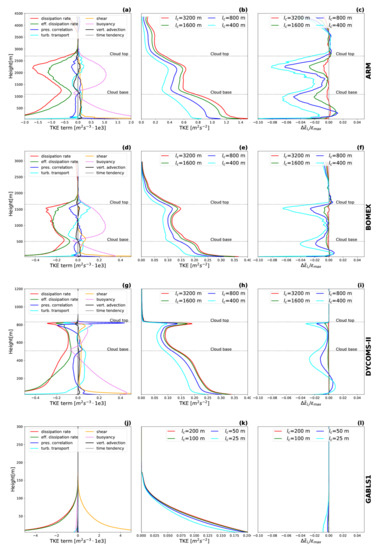
Figure 1.
The TKE budget terms (a,d,g,j), the TKE (b,e,h,k) and the normalized differences in the effective dissipation rate, , (c,f,i,l) for four cases: ARM (first row), BOMEX (second row), DYCOMS-II (third row), and GABLS1 (fourth row). The TKE budget terms are displayed for the smallest sub-domain size, where side of the sub-domain is equal to 1/32 of the side of the whole domain. The TKE and the differences in the effective dissipation rate are displayed for different sub-domain side sizes, .
For comparison, the classical turbulence length scale is estimated in the same manner:
where is assumed to be equal to the effective dissipation rate, , estimated from Equation (22) for the whole domain.
The number and the size of the sub-domains are chosen so that both samples are large enough to ensure the representativeness of the resulting quantities.
Also, LES domain size is chosen large enough to include a sufficient number of sub-domains with spatial scales above the energy production range of TKE. The smallest sub-domains have a spatial scale in the gray zone of turbulence. In this way, the scale dependence of the diagnosed turbulence length scale can be investigated from conventional to gray-zone resolutions.
To verify whether the sub-domains reach into the energy production range, their sizes are compared with the longitudinal integral turbulence length scales (see e.g., [45]):
which is an estimate of the size of the most energetic turbulent eddies. The integral length scales are computed from data of the whole domain, and the integration is done only up to the value where the auto-correlation function falls off to [45].
3.2. LES Simulations
The new length scale diagnostic is tested on four idealized cases, all developed by the Global Energy and Water Cycle Experiment (GEWEX): the drizzling stratocumulus case based on the first research flight (RF01) of the second Dynamics and Chemistry of Marine Stratocumulus (DYCOMS-II) field study [46], the continental cumulus case based on measurements over the Atmospheric Radiation Measurement (ARM) program Cloud and Radiation Testbed (CART) site in Oklahoma [47,48], the trade wind cumulus case based on observations from the Barbados Oceanographic and Meteorological Experiment (BOMEX) [49], and the fourth test case is based on the GEWEX Atmospheric Boundary Layer Study (GABLS1) project [50,51,52].
This relatively diverse set of cases is chosen to demonstrate the capabilities of the new turbulence length scale diagnostic in different ABL regimes. The results can additionally indicate, to what extent the turbulence length scale is case sensitive.
All simulations are performed with the MicroHH LES model [53,54]. MicroHH is setup and run according to the description of the cases. Moist thermodynamics is employed in the simulations for DYCOMS-II, ARM and BOMEX case. The GABLS1 simulation is run with dry thermodynamics. Parametrization of radiation and microphysics is used only in the DYCOMS-II case. These processes are deactivated in the remaining cases.
With the aim of gaining statistics for a wide range of horizontal scales, a relatively large horizontal domain size and high horizontal resolution are used for the LES runs. This enables study of the influence of the horizontal scale on the diagnosed turbulence length scale. The vertical domain size and resolution follow the description and recommendation in their respective inter-comparison studies (while maintaining a physically reasonable aspect ratio of the gird box). The resolutions, the sizes of the domain and the integration time are summarized in Table 1.

Table 1.
Horizontal and vertical domain size, horizontal and vertical resolution, and integration time for the LES runs.
The turbulence length scale is diagnosed on data from rectangular horizontal sub-domains. We construct the sub-domains by decomposing the whole domain into equal squares, with 1, 2, 4, 8, 16, and 32 sub-domains in each direction.
Example of sub-domains construction is displayed in Figure 2.
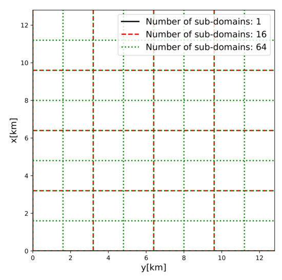
Figure 2.
Example of sub-domains construction.
For the turbulence length scale diagnostic, the TKE budget terms are averaged over all the sub-domains of the same size. The LES statistics are averaged over one hour in time.
All the MicroHH LES simulations reproduce the results of the respective LES inter-comparison studies.
3.3. Fit of Turbulence Length Scale
For demonstration, the diagnosed turbulence length scales are fitted with the following algebraic height-dependent relationship [16,18] :
where is the von Kármán constant, and are closure constants, is the ABL height; and , , and are shape constants. The length scales are fitted with the least-squares method implemented in the scipy Python package. and the shape constants are used as fitting constants. The bounds and the value of the first guess for the fitting constants are presented in Table 2.
Table 2.
First guess and bounds for the fitting constants in Equation (26).
3.4. Computation of Turbulence Fluxes
For illustration, the diagnosed turbulence length scales are used to compute the turbulence fluxes for the GABLS1 case, following the local down-gradient NWP turbulence parametrization of [11]:
where is a closure constant. The flux Richardson number, , the TKE, the potential temperature , and the wind components are obtained by time averaging the corresponding LES data. The turbulence length scale L stands for either the diagnosed turbulence length scale, , or the parametrized turbulence length scale, , according to Equation (18) in [16]. is computed as a minimum of an algebraic [18] and a TKE-based [25] turbulence length scale relationship:
where is given by the balance between TKE and local stability. and are upward and downward free paths, respectively.
3.5. Gravity Waves
The velocity fluctuations in the LES data are caused by both turbulent motions and by gravity waves [15]. The effect of gravity waves is particularly strong above the ABL in the convective cases (BOMEX and ARM). Since it is difficult to separate the TKE from the wave kinetic energy in this region, the estimation of TKE from the LES data is inaccurate. Therefore, we avoid this problematic region in the fitting procedure, and perform the fitting only on data below the cloud top. Cloud top and cloud base are defined in this paper as layers above/under the cloud, where the cloud fraction becomes smaller than .
4. Results
Results of the turbulence length scale diagnostic for the four idealized cases are presented next. We start with the input parameters to the diagnostic: the TKE and the effective dissipation rate (see Equation (23)). The vertical profiles of the sub-gridscale TKE, , and the normalized differences in the effective dissipation rate between the sub-domain and the whole domain, , are presented in Figure 1. The first column in Figure 1 also shows the TKE budget terms for the smallest sub-domain. The changes in the size of the sub-domain are interpreted as changes in the corresponding horizontal grid resolution in an NWP model (see Section 3).
The TKE dissipation rate, , is set to the value of the effective dissipation rate of the whole domain, whose scale is assumed to be above the energy-containing range. The LES data is sampled every 60 s. The LES statistics are obtained by averaging over the last hour of the integration for the ARM, BOMEX, and DYCOMS-II cases. For GABLS1, the LES statistics are obtained by averaging over 45 min after 5 h of integration. To avoid division by zero in the following length scale diagnostic, is limited by a minimal value of , much smaller than the typical values of .
We can see in Figure 1 that the TKE, , gradually decreases with the decreasing size of the sub-domain throughout the entire vertical profile. In comparison, there is more vertical variability in the changes in the effective dissipation rate, because these are dictated by the budget of the TKE. Higher values of source terms and transport terms are usually correlated with stronger changes in . Among the four cases, the GABLS1 case manifests the weakest scale dependence due to relatively low intensity of the TKE source terms. The remaining cases show a similar vertical pattern with increasing horizontal grid resolution for an NWP model: increase of near the surface layer, strong decrease of under the cloud base and under the cloud top, and low scale dependence around the middle of the cloud layer.
The longitudinal integral length scales (see Equation (25)), and , the diagnosed turbulence length scale, , its fit according to Equation (26), , and the parametrized turbulence length scale according to Equation (31), , are presented in Figure 3. The scale dependence of the classical length scale, diagnosed from , (see Equation (24), black and gray lines in Figure 3), is determined solely by changes in TKE. Therefore, the changes in mirror the changes in TKE and are thus relatively uniform with height. is, as expected, a monotonous function of the sub-domain size that converges linearly with to zero (see Equation (24)) for very small sub-domains. The behavior of the new length scale (see Equation (23)) is more complicated, because it depends on two factors, the TKE and . With an increase in resolution, the decrease of increases in comparison with . This effect can even lead to a growth of with increasing resolution. The dependence of on the sub-domain size is thus not always monotonous and can result in local maxima of for a specific resolution within the gray zone. Of course, should ultimately converges to zero for very small sub-domains. Reflecting the changes of , the resolution-dependence of changes with height. Obviously, the biggest differences between and are in the regions where the magnitude of is large: just below the cloud base and the cloud top in the three cloudy cases.
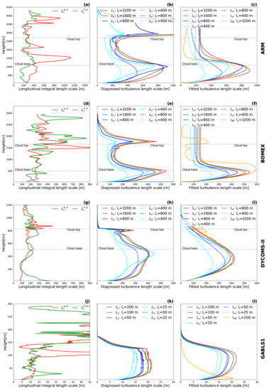
Figure 3.
As in Figure 1, but comparison of the longitudinal integral turbulence length scales (see Equation (25)) for the zonal wind, , and the meridional wind, is computed for the period one hour before the end of the simulation (a,d,g,j); diagnosed turbulence length scales computed from the effective dissipation rate, (see Equation (23)); and the dissipation rate, (see Equation (24)), (b,e,h,k); and their respective fits with the relationship in Equation (26) (c,f,i,l). The parametrized turbulence length scale according to Equation (18) in [16], , is also presented (c,f,i,l). The fits for the ARM and BOMEX cases are done only with data below the cloud top (indicated by horizontal line).
The changes in start to have a significant impact on the turbulence length scale diagnostic from a sub-domain size of 1.6 km × 1.6 km for the cloudy cases and at a sub-domain size of 50 m × 50 m for GABLS1. This can be interpreted as the beginning of the gray zone of turbulence. The largest impact of changes are to be expected at sub-domain sizes around the longitudinal integral length scale, which is approximately 200 m to 400 m for ARM and BOMEX, 100 m to 300 m for DYCOMS-II and 10 m to 30 m for GABLS1. For all cases, the smallest sub-domain sizes are slightly larger than the integral length scales. Hence, all sub-domain sizes are in the upper part of the energy-containing range of TKE, or above it. The setup of the sub-domain is thus suitable for the scale dependence analysis of the upper part of the gray zone.
The influence of makes more variable than , resulting sometimes in atypical vertical profiles compared to a classical turbulence length scale formulation. This is demonstrated via the fitting of with an algebraic height-dependent relationship (see Equation (26)). The fit works very well for the GABLS1 case, where and are very similar. In the cloudy cases, the curvature of the vertical profile of increases with resolution, especially under the cloud base. This strong curvature cannot be completely fitted with the prescribed algebraic formulation.
Additionally, it would be impossible to fit a second peak in the vertical profile of with the chosen algebraic formulation, because the formulation implicitly implies a single-peaked vertical distribution. However, the existence of a second peek under the cloud top in our data is disputable. The presence of gravity waves near the top of the ABL in ARM and BOMEX, make the estimation of TKE and unreliable there (see Section 3.5). The proper resolution of this issue would be to separate the velocity fluctuations caused by gravity waves from the turbulence fluctuations and diagnose arising only from the turbulence part of the flow. This is however beyond the scope of this paper. Therefore, we opt for a pragmatic approach, and we fit only the data under the cloud top for the ARM and BOMEX case. Concerning the DYCOMS-II case, it is well known that most LES models have difficulties in modeling stratocumulus cases, especially near cloud top [55,56]. This is also seen in our simulations. Hence the TKE budget analyses for the DYCOMS-II case near the cloud top is also not reliable. Data from runs with an enhanced LES code could improve the diagnostic of for this case.
The estimation of both and near the cloud top is strongly affected by inaccuracies in the data, because in this region the turbulence length scale is estimated as the ratio of two small numbers. To avoid this problem, the effective dissipation rate or the dissipation rate could be fitted/parametrized in a different way (e.g., direct parametrization without the need for a length or time scale ). This would, however, require a modification of the classical TKE scheme, which is beyond the scope of this paper.
To verify whether the diagnosed turbulence length scale is usable in a NWP turbulence scheme, it is compared with the parametrized turbulence length scale, (see Equation (31)). The diagnosed turbulence length scale for the larger sub-domains has a similar magnitude as . This confirms the validity of the turbulence length scale diagnostic for the NWP scales. There are differences in the shape between and , especially for the GABLS1 case. It is expected that the performance of an NWP turbulence parametrization would improve if or its fit would be used instead of for the computation of the turbulence fluxes (see Equations (27)–(29)). It must be however noted that the turbulence length scale is only one factor in the computation of the turbulence fluxes. The calibration of the closure constants, the shape of the stability functions, the choice of the stability parameter, and the parametrization of non-local effects also influence the quality of the turbulence scheme. Hence, the turbulence scheme should be tested as a whole and should be adjusted if a new turbulence length scale formulation is used. Such modifications are, however, beyond the scope of this paper.
For illustration, and instead of testing the fit of in an NWP parametrization, is used for the computation of the local down-gradient turbulence fluxes according to Equations (27)–(29) directly from the LES data. These fluxes are then compared with the turbulence fluxes computed using and with fluxes obtained directly from LES (see Figure 4) for the GABLS1 case. The cloudy cases are no included, because they would involve an additional parametrization of the non-local turbulence fluxes. The comparison in Figure 4 shows that the fit of and outperforms the parametrized in GABLS1. The turbulence fluxes computed with are in good agreement with the LES fluxes and show a similar scale dependence. As expected, the computed turbulence fluxes are getting smaller for smaller sub-domains, because both the TKE and the turbulence length scale are getting smaller. From the perspective of the NWP parameterization, this corresponds to the increase of the horizontal resolution, where larger turbulence eddies are being resolved. To avoid double counting, the computed sub-grid scale turbulent fluxes should become smaller. The difference between and for the smaller sub-domain (for larger sub-domains they are basically identical) shows that for the decrease of the turbulence fluxes is stronger than for . This is the direct consequence of accounting for the cross-scale TKE transfer in the turbulence length scale diagnostic, which results in a smaller effective dissipation rate weaker in comparison to the dissipation rate.
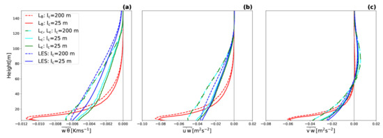
Figure 4.
The turbulent heat flux (a) and the turbulent momentum fluxes (b,c) for GABLS1. The turbulent fluxes are computed according to the local down-gradient formulation (see Equations (27)–(29)) using the fit of the diagnosed turbulent length scale, , (cyan lines), fit of (green lines), or the parametrized turbulence length scale according to Equation (18) in [16], , (red lines) for two sub-domain sizes (dashed lines versus solid lines). The turbulent fluxes acquired directly from LES are plotted with blue lines.
When compared with the LES results, the scale dependence of the turbulent fluxes is too strong for both and . However, the scale dependence caused by is smaller than the scale dependence cause by and is thus closer to the LES results. Quantification of scale dependence is important for future development of a scale-dependent turbulent length scale formulation.
5. Discussion
We have derived and presented a new turbulence length scale diagnostic based on LES data that contains the influence of the sub-grid (in an NWP context) cross-scale TKE transfer. Differently from the classical turbulence length scale, [15], (see Equation (15)) the new turbulence length scale, , is computed from the effective TKE dissipation rate, , instead of the TKE dissipation rate, . The effective dissipation rate takes into account the influence of the cross-scale transfer of TKE from the resolved to the sub-grid scales, which is non-zero in the gray zone of turbulence.
The effective dissipation rate is estimated from the TKE budget (see Section 2). The diagnostic of the associated turbulence length scale, , thus aims directly at the role of the turbulence length scale: parametrization of the TKE loss via dissipation and cross-scale TKE transfer. Thanks to this, does not require other simplified, limiting assumptions, compared to other formulations of the turbulence length scale (see Section 1). Consequently, our new approach offers a better reference for the parametrization of the turbulence length scale in the gray zone of turbulence, where neither the classical NWP or the LES assumptions are applicable. The new diagnostic can thus be used as a basis for a new scale-dependent turbulence length scale formulation suitable for the gray zone of turbulence.
The influence of the cross-scale TKE transfer in the upper part of the gray zone of turbulence on is presented in Section 4 for four LES cases: ARM, BOMEX, DYCOMS-II, and GABLS1. The differences between and basically indicate the largest scales at which the gray zone of turbulence starts to be significant, which in itself could be useful for gray zone detection.
Results in Section 4 show the shape of the vertical profile of varies more strongly with the horizontal scale than the shape of the profile, due to the influence of on .
In the gray zone, the vertical profiles of have thus a rather atypical shape and cannot be fitted with the usual algebraic height-dependent relationships.
To fit the diagnosed values a modification of the algebraic formulations would be required, such as an increase in curvature and possibly the addition of a secondary maxima. We plan to propose a new height-dependent algebraic formulation based on our results in future research. We must however point out that finding a generally valid algebraic formulation, might prove to be difficult, because the properties of are case sensitive. Therefore, this will require a considerable effort and the analyses of more simulations. Another possibility is to use a TKE dependent, or prognostic turbulence length scale formulations [21,22,23,24,25,27] (see Section 1), which correspond better to the actual state of the turbulent flow.
In the gray zone, the turbulence length scale should be a function of the grid resolution. One approach is the blending of an NWP/GC turbulence length scale and a small-scale 3D mixing length scale (see Section 1) [40,41,42]. These methods deliver a turbulence length scale that is a monotonous function of the resolution. The blending is also a height independent procedure. We have shown in Section 4 that the classical turbulence length scale, , is a monotonous function of the resolution and that its scale dependence does not change with height. These two properties are not always valid in the gray zone, as demonstrated by our new turbulence length scale, . This finding should be considered in the design of a new turbulence length scale parametrization in the gray zone of turbulence.
Our method of diagnosing the turbulence length scale for the purpose of NWP parameterization is universal, and should work for any turbulent flow. Nonetheless, the quality of the method is affected by the accuracy of the LES data. Above all, sufficiently large samples need to be used in the computation of the TKE budget terms. For this reason, relatively large horizontal domains and high horizontal resolutions are needed for the LES runs. Reliability of the diagnostic can be additionally affected by gravity waves, as has been discussed in Section 4. Separation of turbulence and gravity waves at the same scale is difficult, but, if possible, this would address the problem of the diagnostic of the turbulence length scale near cloud top for shallow convective cases. It should also be mentioned that LES models have their own inherent limitations. For example modeling of stratocumulus cases is not satisfactory with most LES models. There are proposals to mitigate this problem [55,56], and we would like to test data produced with such an enhanced LES code.
We have demonstrated that the fit of the diagnosed turbulence length scale has similar magnitudes as the parametrized turbulence length scale according to [16] (see Figure 3) and it performs well in a local down-gradient turbulence flux computation (see Figure 4). However, to assess the added value of the new turbulence length scale formulations, it needs to be tested in a full NWP parametrization.
Author Contributions
Conceptualization, I.B.Ď., J.S. and R.B.; methodology, I.B.Ď., J.S. and R.B.; software, I.B.Ď.; validation, I.B.Ď.; formal analysis, I.B.Ď.; investigation, I.B.Ď., J.S. and R.B.; resources, J.S. and I.B.Ď.; data curation, I.B.Ď.; writing—original draft preparation, I.B.Ď.; writing—review and editing, I.B.Ď., J.S. and R.B.; visualization, I.B.Ď.; project administration, I.B.Ď. and J.S.; funding acquisition, J.S. and I.B.Ď. All authors have read and agreed to the published version of the manuscript.
Funding
This research was funded by Hans Ertel Centre for Weather Research of DWD (3rd phase, The Atmospheric Boundary Layer in Numerical Weather Prediction) grant number 4818DWDP4. Ritthik Bhattacharya was supported by Meteo Swiss.
Acknowledgments
The authors would like to thank Chiel C. van Heerwaarden and T. J. Anurose who helped as technical support with running the LES code. The data for this study were generated with the LES model MicroHH, openly available in Zenodo at https://doi.org/10.5281/zenodo.822842 [54]. The configuration files and output statistics of the four simulations (ARM, BOMEX, GABLS1, and DYCMS-II) are openly available in Zenodo at https://doi.org/10.5281/zenodo.3685801 [57]. The simulations were performed on MISTRAL, DKRZ, Hamburg, Germany.
Conflicts of Interest
The authors declare no conflict of interest. The funders had no role in the design of the study; in the collection, analyses, or interpretation of data; in the writing of the manuscript, or in the decision to publish the results.
Abbreviations
The following abbreviations are used in this manuscript:
| ABL | Atmospheric Boundary Layer |
| ARM | Atmospheric Radiation Measurement |
| BOMEX | Barbados Oceanographic and Meteorological Experiment |
| DYCOMS-II | second Dynamics and Chemistry of Marine Stratocumulus |
| GABLS | GEWEX Atmospheric Boundary Layer Study |
| GC | Global Circulation |
| LES | Large Eddy Simulation |
| NWP | Numerical Weather Prediction |
| TKE | Turbulence Kinetic Energy |
References
- Wyngaard, J.C. Toward Numerical Modeling in the “Terra Incognita”. J. Atmos. Sci. 2004, 61, 1816–1826. [Google Scholar] [CrossRef]
- Honnert, R.; Masson, V.; Couvreux, F. A Diagnostic for Evaluating the Representation of Turbulence in Atmospheric Models at the Kilometric Scale. J. Atmos. Sci. 2011, 68, 3112–3131. [Google Scholar] [CrossRef]
- Honnert, R. Representation of the grey zone of turbulence in the atmospheric boundary layer. Adv. Sci. Res. 2016, 13, 63–67. [Google Scholar] [CrossRef]
- Stull, R.B. An Introduction to Boundary Layer Meteorology; Kluwer Academic Publishers: Amsterdam, The Netherlands, 1988. [Google Scholar]
- Mellor, G.L.; Yamada, T. A Hierarchy of Turbulence Closure Models for Planetary Boundary Layers. J. Atmos. Sci. 1974, 31, 1791–1806. [Google Scholar] [CrossRef]
- Golaz, J.C.; Larson, V.E.; Cotton, W.R. A PDF-Based Model for Boundary Layer Clouds. Part I: Method and Model Description. J. Atmos. Sci. 2002, 59, 3540–3551. [Google Scholar] [CrossRef]
- Mironov, D.V.; Machulskaya, E. A Turbulence Kinetic Energy—Scalar Variance Turbulence Parameterization Scheme. 2017. Available online: www.cosmo-model.org (accessed on 18 April 2020).
- Mellor, G.L.; Yamada, T. Development of a turbulence closure model for geophysical fluid problems. Rev. Geophys. 1982, 20, 851–875. [Google Scholar] [CrossRef]
- Redelsperger, J.L.; Mahé, F.; Carlotti, P. A Simple And General Subgrid Model Suitable Both For Surface Layer And Free-Stream Turbulence. Bound.-Layer Meteorol. 2001, 101, 375–408. [Google Scholar] [CrossRef]
- Cheng, Y.; Canuto, V.; Howard, A. An Improved Model for the Turbulent PBL. J. Atmos. Sci. 2002, 59, 1550–1565. [Google Scholar] [CrossRef]
- Bašták Ďurán, I.; Geleyn, J.F.; Váňa, F. A Compact Model for the Stability Dependency of TKE Production-Destruction-Conversion Terms Valid for the Whole Range of Richardson Numbers. J. Atmos. Sci. 2014, 71, 3004–3026. [Google Scholar] [CrossRef]
- Lenderink, G.; Holtslag, A.A.M. An updated length-scale formulation for turbulent mixing in clear and cloudy boundary layers. Q. J. R. Meteorol. Soc. 2004, 130, 3405–3427. [Google Scholar] [CrossRef]
- Sáanchez, E.; Cuxart, J. A buoyancy-based mixing-length proposal for cloudy boundary layers. Q. J. R. Meteorol. Soc. 2004, 130, 3385–3404. [Google Scholar] [CrossRef]
- Nakanishi, M. Improvement of the Mellor–Yamada Turbulence Closure Model Based on Large-Eddy Simulation Data. Bound.-Layer Meteorol. 2001, 99, 349–378. [Google Scholar] [CrossRef]
- Kitamura, Y. Estimating Dependence of the Turbulent Length Scales on Model Resolution Based on a Priori Analysis. J. Atmos. Sci. 2015, 72, 750–762. [Google Scholar] [CrossRef]
- Bašták Ďurán, I.; Geleyn, J.F.; Váňa, F.V.; Schmidli, J.; Brožková, R. A Turbulence Scheme with Two Prognostic Turbulence Energies. J. Atmos. Sci. 2018, 75, 3381–3402. [Google Scholar] [CrossRef]
- Blackadar, A.K. The vertical distribution of wind and turbulent exchange in a neutral atmosphere. J. Geophys. Res. (1896–1977) 1962, 67, 3095–3102. [Google Scholar] [CrossRef]
- Cedilnik, J. Parallel Suites Documentation. 2005. Available online: http://www.https.com//www.rclace.eu/file/physics/2005 (accessed on 18 April 2020).
- Von Karman, T. Mechanische Ähnlichkeit und Turbulenz. Nachr. Ges. Wiss. Göttingen 1930, 58–76, also Proceedings of the Third International Congress of Applied Mechanics. Stockholm 1930. [Google Scholar]
- Prandtl, L. Zur turbulenten Stromung in Rohren und langs Platten. Ergebnisse der Aerodynamischen Versuchsanstalt zu GöTtingen 1932, 4, 18–29. [Google Scholar]
- Deardorff, J.W. Stratocumulus-capped mixed layers derived from a three-dimensional model. Bound.-Layer Meteorol. 1980, 18, 495–527. [Google Scholar] [CrossRef]
- Teixeira, J.; Cheinet, S. A Simple Mixing Length Formulation for the Eddy-Diffusivity Parameterization of Dry Convection. Bound.-Layer Meteorol. 2004, 110, 435–453. [Google Scholar] [CrossRef]
- Nakanishi, M.; Niino, H. Development of an Improved Turbulence Closure Model for the Atmospheric Boundary Layer. J. Meteorol. Soc. Jpn. Ser. II 2009, 87, 895–912. [Google Scholar] [CrossRef]
- Bogenschutz, P.A.; Krueger, S.K. A simplified PDF parameterization of subgrid-scale clouds and turbulence for cloud-resolving models. J. Adv. Model. Earth Syst. 2013, 5, 195–211. [Google Scholar] [CrossRef]
- Bougeault, P.; Lacarrere, P. Parameterization of Orography-Induced Turbulence in a Mesobeta–Scale Model. Mon. Weather Rev. 1989, 117, 1872–1890. [Google Scholar] [CrossRef]
- Kantha, L.H. The length scale equation in turbulence models. Nonlinear Process. Geophys. 2004, 11, 83–97. [Google Scholar] [CrossRef]
- Zilitinkevich, S.; Elperin, T.; Kleeorin, N.; Rogachevskii, I.; Esau, I. A Hierarchy of Energy- and Flux-Budget (EFB) Turbulence Closure Models for Stably-Stratified Geophysical Flows. Bound.-Layer Meteor. 2013, 146, 341–373. [Google Scholar] [CrossRef]
- Wyngaard, J.C. Turbulence in the Atmosphere; Cambridge University Press: Cambridge, UK, 2010. [Google Scholar] [CrossRef]
- Kolmogorov, A. The local structure of turbulence in incompressible viscous fluid for very large Reynolds numbers. Proc. USSR Acad. Sci. 1941, 30, 299–303. (In Russian) [Google Scholar]
- de Roode, S.R.; Duynkerke, P.G.; Jonker, H.J.J. Large-Eddy Simulation: How Large is Large Enough? J. Atmos. Sci. 2004, 61, 403–421. [Google Scholar] [CrossRef]
- Cuxart, J.; Bougeault, P.; Redelsperger, J.L. A turbulence scheme allowing for mesoscale and large-eddy simulations. Q. J. R. Meteorol. Soc. 2000, 126, 1–30. [Google Scholar] [CrossRef]
- Peña, A.; Gryning, S.E.; Mann, J. On the length-scale of the wind profile. Q. J. R. Meteorol. Soc. 2010, 136, 2119–2131. [Google Scholar] [CrossRef]
- Weinstock, J. On the Theory of Turbulence in the Buoyancy Subrange of Stably Stratified Flows. J. Atmos. Sci. 1978, 35, 634–649. [Google Scholar] [CrossRef]
- Cheng, Y.; Li, Q.; Argentini, S.; Sayde, C.; Gentine, P. Turbulence Spectra in the Stable Atmospheric Boundary Layer. arXiv 2018, arXiv:1801.05847v3. [Google Scholar]
- O’Connor, E.J.; Illingworth, A.J.; Brooks, I.M.; Westbrook, C.D.; Hogan, R.J.; Davies, F.; Brooks, B.J. A Method for Estimating the Turbulent Kinetic Energy Dissipation Rate from a Vertically Pointing Doppler Lidar, and Independent Evaluation from Balloon-Borne In Situ Measurements. J. Atmos. Ocean. Technol. 2010, 27, 1652–1664. [Google Scholar] [CrossRef]
- Hatlee, S.C.; Wyngaard, J.C. Improved Subfilter-Scale Models from the HATS Field Data. J. Atmos. Sci. 2007, 64, 1694–1705. [Google Scholar] [CrossRef]
- Zhou, B.; Zhu, K.; Xue, M. A Physically Based Horizontal Subgrid-Scale Turbulent Mixing Parameterization for the Convective Boundary Layer. J. Atmos. Sci. 2017, 74, 2657–2674. [Google Scholar] [CrossRef]
- Zhang, X.; Bao, J.W.; Chen, B.; Grell, E.D. A Three-Dimensional Scale-Adaptive Turbulent Kinetic Energy Scheme in the WRF-ARW Model. Mon. Weather Rev. 2018, 146, 2023–2045. [Google Scholar] [CrossRef]
- Bhattacharya, R.; Stevens, B. A two Turbulence Kinetic Energy model as a scale-adaptive approach to modeling the planetary boundary layer. J. Adv. Model. Earth Syst. 2016, 8, 224–243. [Google Scholar] [CrossRef]
- Boutle, I.A.; Eyre, J.E.J.; Lock, A.P. Seamless Stratocumulus Simulation across the Turbulent Gray Zone. Mon. Weather Rev. 2014, 142, 1655–1668. [Google Scholar] [CrossRef]
- Efstathiou, G.A.; Beare, R.J. Quantifying and improving sub-grid diffusion in the boundary-layer grey zone. Q. J. R. Meteorol. Soc. 2015, 141, 3006–3017. [Google Scholar] [CrossRef]
- Kurowski, M.J.; Teixeira, J. A Scale-Adaptive Turbulent Kinetic Energy Closure for the Dry Convective Boundary Layer. J. Atmos. Sci. 2018, 75, 675–690. [Google Scholar] [CrossRef]
- Lilly, D. The representation of small-scale turbulence in numerical simulation experiments. In Proceedings of the IBM Scientific Computing Symposium on Environmental Sciences, New York, NY, USA, 14–16 November 1967; pp. 195–210. [Google Scholar]
- Heinze, R.; Mironov, D.; Raasch, S. Second-moment budgets in cloud topped boundary layers: A large-eddy simulation study. J. Adv. Model. Earth Syst. 2015, 7, 510–536. [Google Scholar] [CrossRef]
- O’Neill, P.; Nicolaides, D.; Honnery, D.; Soria, J. Autocorrelation functions and the determination of integral length with reference to experimental and numerical data. In Proceedings of the Fifteenth Australasian Fluid Mechanics Conference, Sydney, Australia, 13–17 December 2004; Behnia, M., Lin, W., McBain, G., Eds.; The University of Sydney: Sydney, Australia, 2004; pp. 1–4. [Google Scholar]
- Stevens, B.; Moeng, C.H.; Ackerman, A.S.; Bretherton, C.S.; Chlond, A.; de Roode, S.; Edwards, J.; Golaz, J.C.; Jiang, H.; Khairoutdinov, M.; et al. Evaluation of Large-Eddy Simulations via Observations of Nocturnal Marine Stratocumulus. Mon. Weather Rev. 2005, 133, 1443–1462. [Google Scholar] [CrossRef]
- Brown, A.R.; Cederwall, R.T.; Chlond, A.; Duynkerke, P.G.; Golaz, J.C.; Khairoutdinov, M.; Lewellen, D.C.; Lock, A.P.; MacVean, M.K.; Moeng, C.H.; et al. Large-eddy simulation of the diurnal cycle of shallow cumulus convection over land. Q. J. R. Meteorol. Soc. 2002, 128, 1075–1093. [Google Scholar] [CrossRef]
- Lenderink, G.; Siebesma, A.P.; Cheinet, S.; Irons, S.; Jones, C.G.; Marquet, P.; Müller, F.M.; Olmeda, D.; Calvo, J.; Sánchez, E.; et al. The diurnal cycle of shallow cumulus clouds over land: A single-column model intercomparison study. Q. J. R. Meteorol. Soc. 2004, 130, 3339–3364. [Google Scholar] [CrossRef]
- Siebesma, A.P.; Bretherton, C.S.; Brown, A.; Chlond, A.; Cuxart, J.; Duynkerke, P.G.; Jiang, H.; Khairoutdinov, M.; Lewellen, D.; Moeng, C.H.; et al. A Large Eddy Simulation Intercomparison Study of Shallow Cumulus Convection. J. Atmos. Sci. 2003, 60, 1201–1219. [Google Scholar] [CrossRef]
- Holtslag, B. Preface: GEWEX Atmospheric Boundary-layer Study (GABLS) on Stable Boundary Layers. Bound.-Layer Meteorol. 2006, 118, 243–246. [Google Scholar] [CrossRef]
- Beare, R.J.; Macvean, M.K.; Holtslag, A.A.M.; Cuxart, J.; Esau, I.; Golaz, J.C.; Jimenez, M.A.; Khairoutdinov, M.; Kosovic, B.; Lewellen, D.; et al. An Intercomparison of Large-Eddy Simulations of the Stable Boundary Layer. Bound.-Layer Meteorol. 2006, 118, 247–272. [Google Scholar] [CrossRef]
- Cuxart, J.; Holtslag, A.A.M.; Beare, R.J.; Bazile, E.; Beljaars, A.; Cheng, A.; Conangla, L.; Ek, M.; Freedman, F.; Hamdi, R.; et al. Single-Column Model Intercomparison for a Stably Stratified Atmospheric Boundary Layer. Bound.-Layer Meteorol. 2006, 118, 273–303. [Google Scholar] [CrossRef]
- van Heerwaarden, C.C.; van Stratum, B.J.H.; Heus, T.; Gibbs, J.A.; Fedorovich, E.; Mellado, J.P. MicroHH 1.0: A computational fluid dynamics code for direct numerical simulation and large-eddy simulation of atmospheric boundary layer flows. Geosci. Model Dev. 2017, 10, 3145–3165. [Google Scholar] [CrossRef]
- van Heerwaarden, C.; van Stratum, B.; Heus, T. microhh/microhh: 1.0.0. Zenodo 2017. [Google Scholar] [CrossRef]
- Pressel, K.G.; Mishra, S.; Schneider, T.; Kaul, C.M.; Tan, Z. Numerics and subgrid-scale modeling in large eddy simulations of stratocumulus clouds. J. Adv. Model. Earth Syst. 2017, 9, 1342–1365. [Google Scholar] [CrossRef]
- Shi, X.; Enriquez, R.M.; Street, R.L.; Bryan, G.H.; Chow, F.K. An Implicit Algebraic Turbulence Closure Scheme for Atmospheric Boundary Layer Simulation. J. Atmos. Sci. 2019, 76, 3367–3386. [Google Scholar] [CrossRef]
- Bastak Duran, I.; Schmidli, J.; Bhattacharya, R. Data for A budget-based turbulence length scale diagnostic. Zenodo 2020. [Google Scholar] [CrossRef]
© 2020 by the authors. Licensee MDPI, Basel, Switzerland. This article is an open access article distributed under the terms and conditions of the Creative Commons Attribution (CC BY) license (http://creativecommons.org/licenses/by/4.0/).