Projecting Changes in Temperature Extremes in the Han River Basin of China Using Downscaled CMIP5 Multi-Model Ensembles


Abstract
1. Introduction
2. Data and Methods
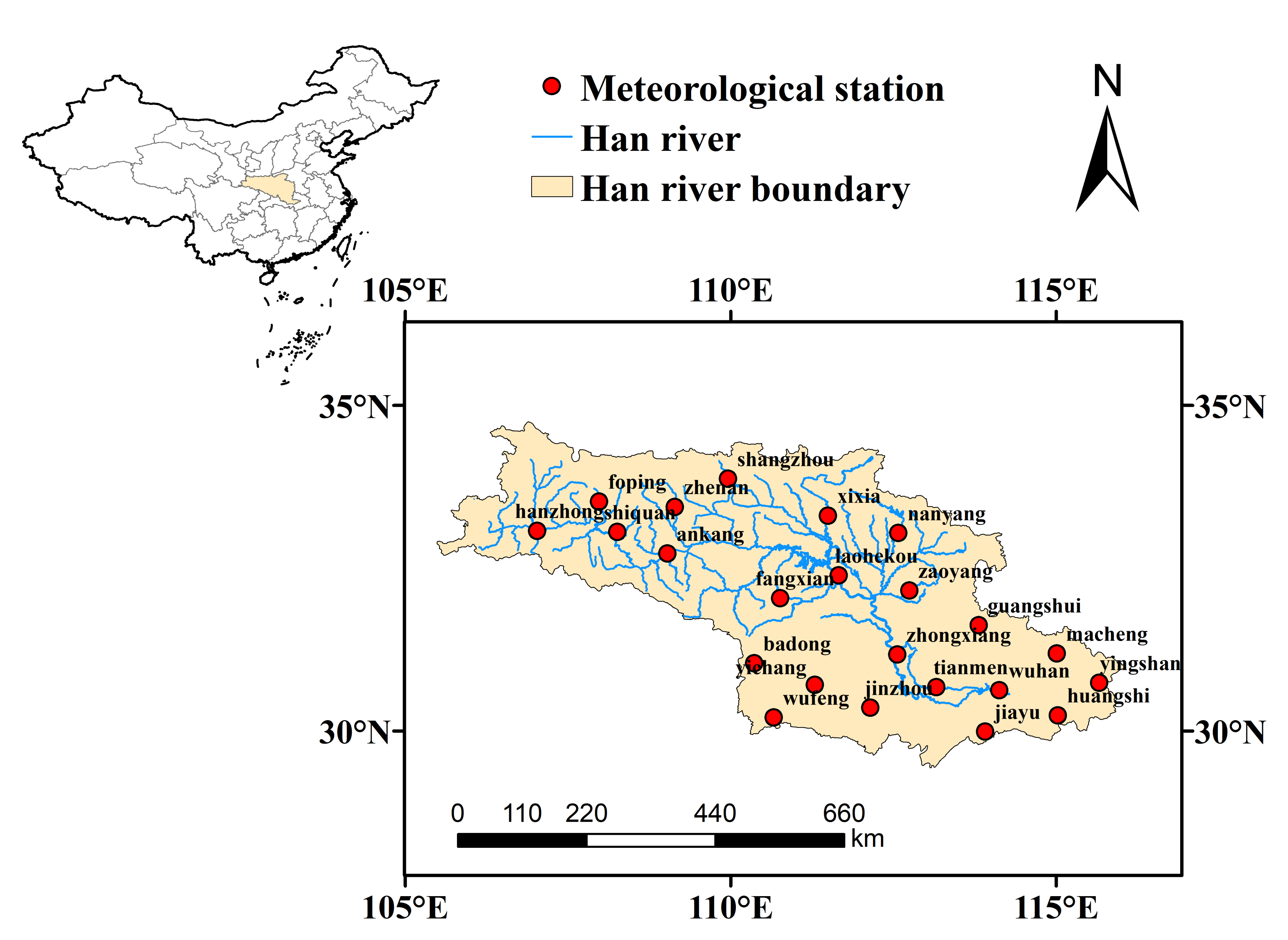
2.1. Study Area
2.2. Climate Data
2.3. Extreme Temperature Indices
2.4. Statistical Analysis
3. Results
3.1. Comparison between Observed and Projected Temperature Extremes during the Historical Period
3.2. Projected Changes of Temperature Extremes by Multi-Model Ensembles in the Future
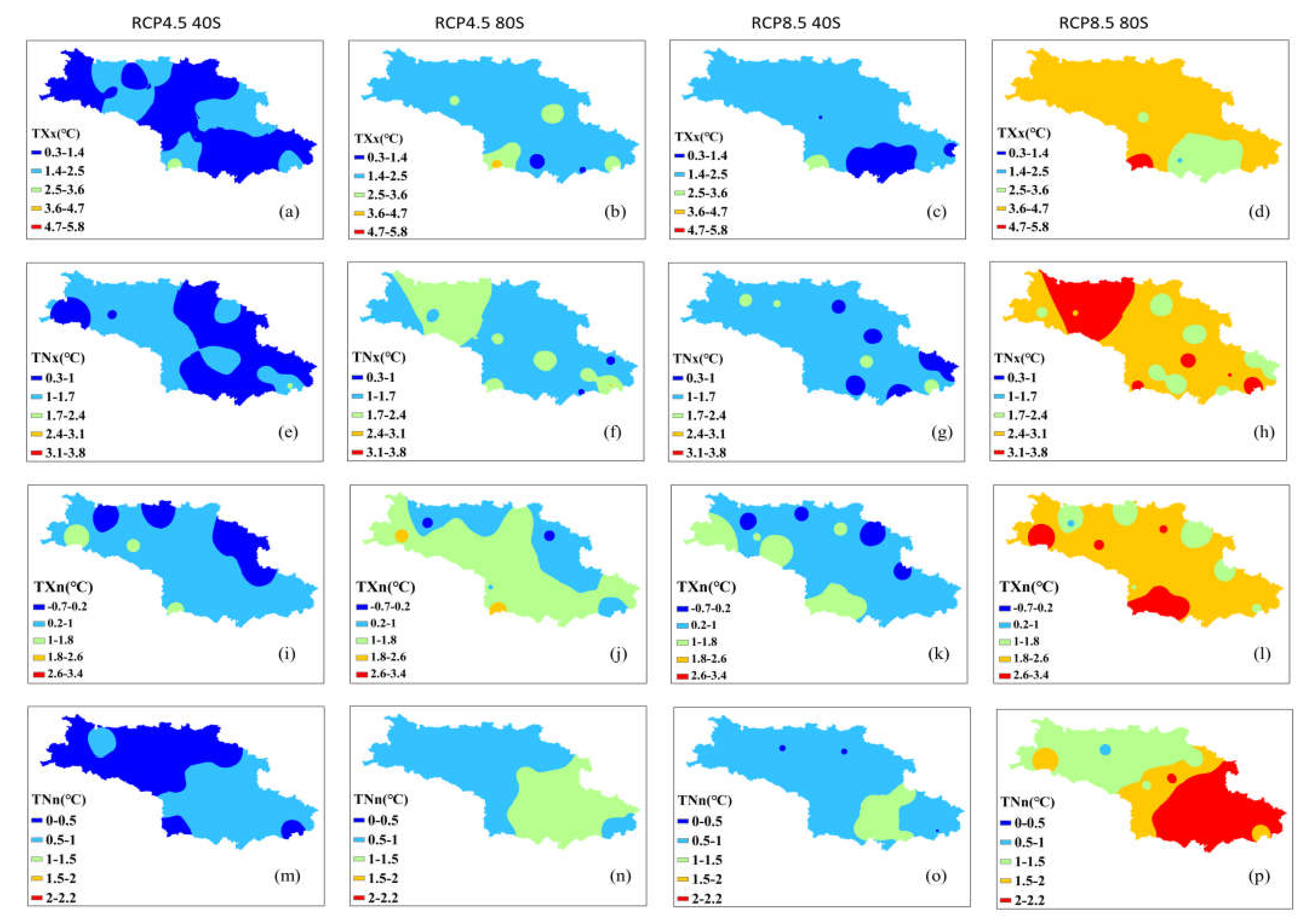
3.2.1. Projected Changes in the Four Intensity-Based Extreme Indices (TXx, TNx, TNn, TXn)
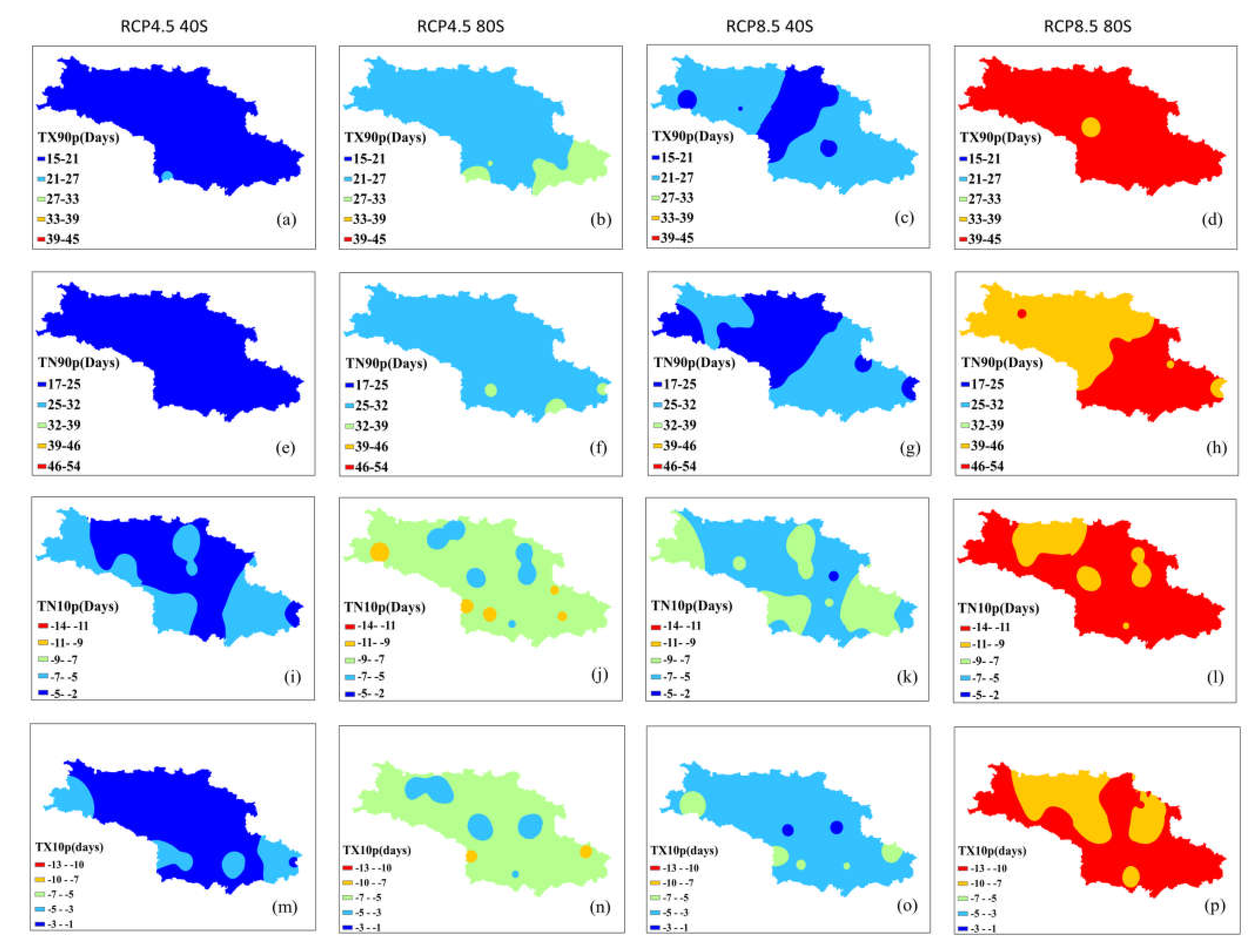
3.2.2. Projected Changes in the Four Percentile-Based Indices
3.2.3. Projected Changes in Four Spell Duration Indices
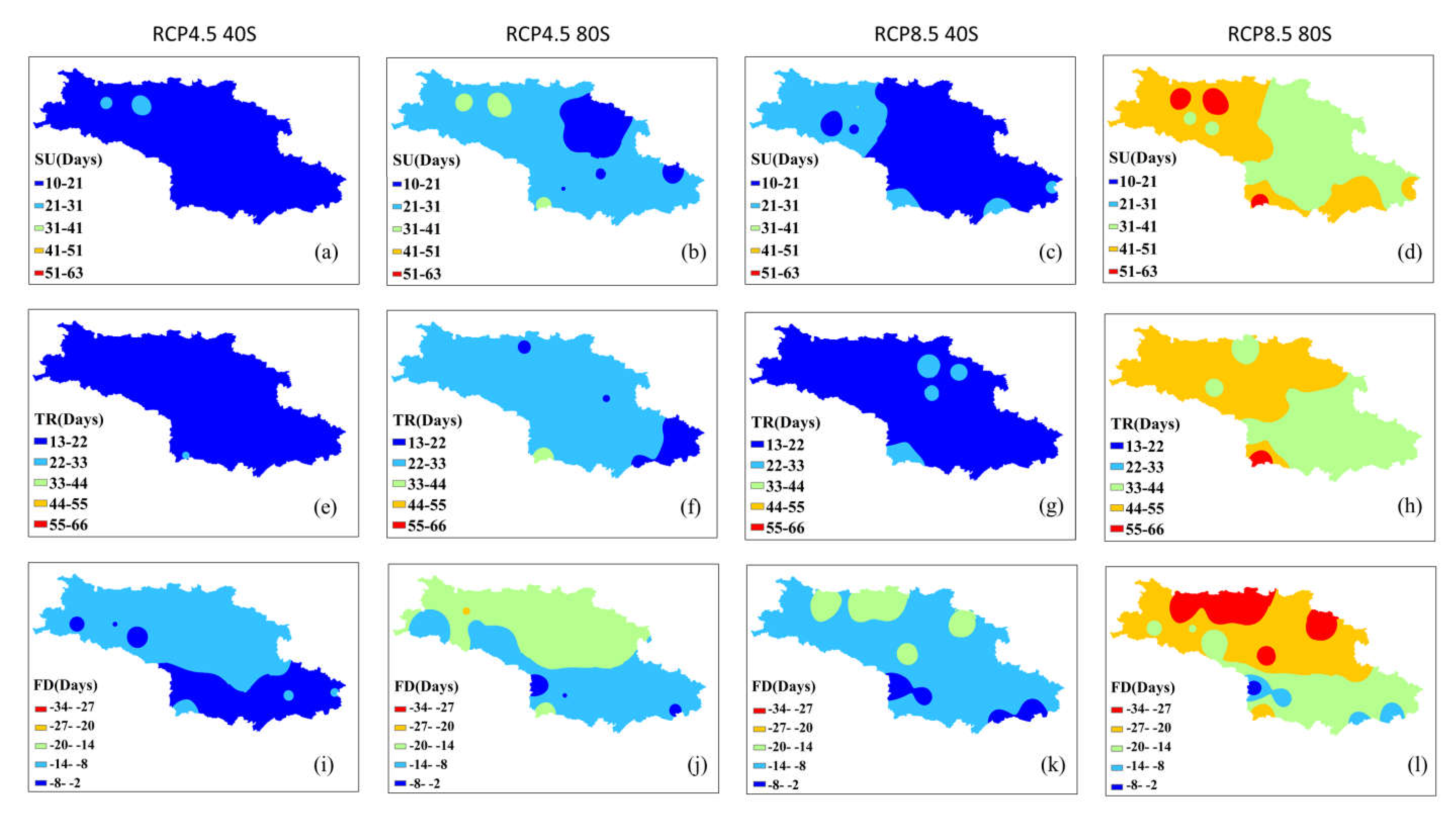
3.2.4. Future Changes in Four Fixed Threshold-Based Indices
4. Discussion
5. Conclusions
Supplementary Materials
Author Contributions
Funding
Acknowledgments
Conflicts of Interest
References
- Field, C.; Barros, V.; Stocker, T. Managing the risks of extreme events and disasters to advance climate change adaptation:Special report of the Intergovernmental Panel on Climate Change. J. Clin. Endocrinol. Metab. 2012, 18, 586–599. [Google Scholar]
- Fischer, E.M.; Knutti, R. Anthropogenic contribution to global occurrence of heavy-precipitation and high-temperature extremes. Nat. Clim. Chang. 2015, 5, 560–564. [Google Scholar] [CrossRef]
- IPCC. Climate Change 2013: The Physical Science Basis. Fifth Assessment Report of the Intergovernmental Panel Contribution of Working Group on Climate Change; Cambridge University Press: Cambridge, UK, 2013. [Google Scholar]
- Zhang, G.; Dong, J.; Zhou, C.; Xu, X.; Min, W.; Hua, O.; Xiao, X. Increasing cropping intensity in response to climate warming in Tibetan Plateau, China. Field Crop. Res. 2013, 142, 36–46. [Google Scholar] [CrossRef]
- Wang, B.; Liu, D.L.; Macadam, I.; Alexander, L.V.; Abramowitz, G.; Yu, Q. Multi-model ensemble projections of future extreme temperature change using a statistical downscaling method in south eastern Australia. Clim. Chang. 2016, 138, 85–98. [Google Scholar] [CrossRef]
- Allen, M.R.; Ingram, W.J. Constraints on future changes in climate and the hydrologic cycle. Nature 2002, 419, 228–232. [Google Scholar] [CrossRef] [PubMed]
- Easterling, D.R.; Meehl, G.A.; Parmesan, C.; Changnon, S.A.; Karl, T.R.; Mearns, L.O. Climate extremes: Observations, modeling, and impacts. Science 2000, 289, 2068–2074. [Google Scholar] [CrossRef] [PubMed]
- Alexander, L.V.; Zhang, X.; Peterson, T.C.; Caesar, J.; Gleason, B.; Tank, A.M.G.K.; Haylock, M.; Collins, D.; Trewin, B.; Rahimzadeh, F. Global observed changes in daily climate extremes of temperature and precipitation. J. Geophys. Res. Atmos. 2006, 111, 1042–1063. [Google Scholar] [CrossRef]
- Kharin, V.V.; Zwiers, F.; Zhang, X.; Wehner, M. Changes in temperature and precipitation extremes in the CMIP5 ensemble. Clim. Chang. 2013, 119, 345–357. [Google Scholar] [CrossRef]
- Schoof, J.T.; Robeson, S.M. Projecting changes in regional temperature and precipitation extremes in the United States. Weather Clim. Extrem. 2016, 11, 28–40. [Google Scholar] [CrossRef]
- Alexander, L.V.; Arblaster, J.M. Historical and projected trends in temperature and precipitation extremes in Australia in observations and CMIP5. Weather Clim. Extrem. 2017, 15, 34–56. [Google Scholar] [CrossRef]
- Nikulin, G.; Kjellström, E.; Hansson, U.; Strandberg, G.; Ullerstig, A. Evaluation and future projections of temperature, precipitation and wind extremes over Europe in an ensemble of regional climate simulations. Tellus 2011, 63, 41–55. [Google Scholar] [CrossRef]
- Shi, C.; Jiang, Z.-H.; Chen, W.-L.; Li, L. Changes in temperature extremes over China under 1.5 °C and 2 °C global warming targets. Adv. Clim. Chang. Res. 2018, 9, 120–129. [Google Scholar] [CrossRef]
- Tian, J.; Liu, J.; Wang, J.; Li, C.; Nie, H.; Yu, F. Trend analysis of temperature and precipitation extremes inmajor grain producing area of China. Int. J. Climatol. 2016, 37, 672–687. [Google Scholar] [CrossRef]
- Yang, T.; Li, H.; Wang, W.; Xu, C.Y.; Yu, Z. Statistical downscaling of extreme daily precipitation, evaporation, and temperature and construction of future scenarios. Hydrol. Process. 2012, 26, 3510–3523. [Google Scholar] [CrossRef]
- Li, L.; Yao, N.; Li, Y.; Liu, D.L.; Wang, B.; Ayantobo, O.O. Future projections of extreme temperature events in different sub-regions of China. Atmos. Res. 2019, 217, 150–164. [Google Scholar] [CrossRef]
- He, L.; Cleverly, J.; Wang, B.; Jin, N.; Mi, C.; Liu, D.L.; Yu, Q. Multi-model ensemble projections of future extreme heat stress on rice across southern China. Theor. Appl. Climatol. 2018, 133, 1107–1118. [Google Scholar] [CrossRef]
- Kang, L.; Peng, B.; Li, J.; Liu, C. Variability of temperature extremes in the Yellow River basin during 1961–2011. Quat. Int. 2014, 336, 52–64. [Google Scholar]
- Guan, Y.; Zhang, X.; Zheng, F.; Wang, B. Trends and variability of daily temperature extremes during 1960–2012 in the Yangtze River Basin, China. Glob. Planet. Chang. 2015, 124, 79–94. [Google Scholar] [CrossRef]
- Miao, C.; Xi, Y.; Wu, J.; Duan, Q.; Lei, X.; Li, H. Spatiotemporal changes in extreme temperature and precipitation events in the Three-Rivers Headwater region, China. J. Geophys. Res. Atmos. 2018, 123, 5827–5844. [Google Scholar]
- Zhao, Y.; Zou, X.; Cao, L.; Xu, X. Changes in precipitation extremes over the Pearl River Basin, southern China, during 1960–2012. Quat. Int. 2014, 333, 26–39. [Google Scholar] [CrossRef]
- Liu, S.; Huang, S.; Xie, Y.; Qiang, H.; Leng, G.; Hou, B.; Ying, Z.; Xiu, W. Spatial-temporal changes of maximum and minimum temperatures in the Wei River Basin, China: Changing patterns, causes and implications. Atmos. Res. 2018, 204, 1–11. [Google Scholar] [CrossRef]
- Nie, C.J.; Li, H.R.; Yang, L.S.; Ye, B.X.; Dai, E.F.; Wu, S.H.; Liu, Y.; Liao, Y.F. Spatial and temporal changes in extreme temperature and extreme precipitation in Guangxi. Quat. Int. 2012, 263, 162–171. [Google Scholar] [CrossRef]
- Taylor, K.E.; Stouffer, R.J.; Meehl, G.A. An overview of CMIP5 and the Experiment Design. Bull. Am. Meteorol. Soc. 2012, 93, 485–498. [Google Scholar] [CrossRef]
- Zhou, B.; Wen, Q.H.; Xu, Y.; Song, L.; Zhang, X. Projected Changes in Temperature and Precipitation Extremes in China by the CMIP5 Multimodel Ensembles. J. Clim. 2014, 27, 6591–6611. [Google Scholar] [CrossRef]
- Wang, X.; Yang, T.; Li, X.; Shi, P.; Zhou, X. Spatio-temporal changes of precipitation and temperature over the Pearl River basin based on CMIP5 multi-model ensemble. Stoch. Environ. Res. Risk Assess. 2017, 31, 1077–1089. [Google Scholar] [CrossRef]
- Xue, Y.; Vasic, R.; Janjic, Z.; Mesinger, F.; Mitchell, K.E. Assessment of Dynamic Downscaling of the Continental U.S. Regional Climate Using the Eta/SSiB Regional Climate Model. J. Clim. 2007, 20, 4172–4193. [Google Scholar] [CrossRef]
- Guo, J.; Huang, G.; Wang, X.; Li, Y.; Lin, Q. Dynamically-downscaled projections of changes in temperature extremes over China. Clim. Dyn. 2018, 50, 1045–1066. [Google Scholar] [CrossRef]
- Ayar, P.V.; Vrac, M.; Bastin, S.; Carreau, J.; Déqué, M.; Gallardo, C. Intercomparison of statistical and dynamical downscaling models under the EURO- and MED-CORDEX initiative framework: Present climate evaluations. Clim. Dyn. 2016, 46, 1301–1329. [Google Scholar] [CrossRef]
- Wilby, R.L.; Dawson, C.W.; Barrow, E.M. Sdsm—A decision support tool for the assessment of regional climate change impacts. Environ. Model. Softw. 2002, 17, 145–157. [Google Scholar] [CrossRef]
- Chen, Y.D.; Li, J.; Zhang, Q. Changes in site-scale temperature extremes over China during 2071–2100 in CMIP5 simulations. J. Geophys. Res. Atmos. 2016, 121, 2732–2749. [Google Scholar] [CrossRef]
- Li, Z.; Zheng, F.-L.; Liu, W.-Z.; Jiang, D.-J. Spatially downscaling GCMs outputs to project changes in extreme precipitation and temperature events on the Loess Plateau of China during the 21st Century. Glob. Planet. Chang. 2012, 82, 65–73. [Google Scholar] [CrossRef]
- Chen, Y.D.; Li, J.; Zhang, Q.; Gu, X. Projected changes in seasonal temperature extremes across China from 2017 to 2100 based on statistical downscaling. Glob. Planet. Chang. 2018, 166, 30–40. [Google Scholar] [CrossRef]
- Qi, W.; Li, H.; Zhang, Q.; Zhang, K. Forest restoration efforts drive changes in land-use/land-cover and water-related ecosystem services in China’s Han River basin. Ecol. Eng. 2019, 126, 64–73. [Google Scholar] [CrossRef]
- Ren, L.; Yin, S. Temperature Changes and its Impacts on Agriculture in the upper Reaches of Hanjiang River in Southern Shaanxi. Chin. J. Agrometeorol. 2013, 34, 272–277. [Google Scholar]
- Zhao, J.; Yang, X.; Xu, Y.; Zhou, Q. Research on the Variation of Extreme Temperature Index in Ankang, Shaanxi in Recent 50 Years. J. Catastrophol. 2016, 31, 89–94. [Google Scholar]
- Xiang, W.; Cheng, Z.; Zhou, B.; Bin, X.; Feng, D. Spatial heterogeneity of temperature extremes in the Qinling-Daba Mountains region in 1975–2016. Clim. Chang. Res. 2018, 14, 362–370. [Google Scholar]
- Liu, W.; Liu, G.; Liu, H.; Song, Y.; Zhang, Q. Subtropical reservoir shorelines have reduced plant species and functional richness compared with adjacent riparian wetlands. Environ. Res. Lett. 2013, 8, 4007. [Google Scholar] [CrossRef]
- Cai, S.; Chen, G.; Du, Y.; Wu, Y. Thoughts on sustainable development in the basin of Hanjiang River. Resour. Environ. Yangtze Basin 2000, 9, 411–418. [Google Scholar]
- Liu, D.L.; Zuo, H. Statistical downscaling of daily climate variables for climate change impact assessment over New South Wales, Australia. Clim. Chang. 2012, 115, 629–666. [Google Scholar] [CrossRef]
- Zhang, H.; Wang, B.; Zhang, M.; Feng, P.; Cheng, L.; Yu, Q.; Eamus, D. Impacts of future climate change on water resource availability of eastern Australia. J. Hydrol. 2019, 573, 49–59. [Google Scholar] [CrossRef]
- Kendall, M.G. Rank Correlation Methods; Charles Griffin: London, UK, 1975. [Google Scholar]
- Mann, H.B. Nonparametric tests against trend. Econometrica 1945, 13, 245–259. [Google Scholar] [CrossRef]
- Sen, P.K. Estimates of the Regression Coefficient Based on Kendall’s Tau. Publ. Am. Stat. Assoc. 1968, 63, 1379–1389. [Google Scholar] [CrossRef]
- Sang, Y.-F.; Wang, Z.; Liu, C. Spatial and temporal variability of daily temperature during 1961–2010 in the Yangtze River Basin, China. Quat. Int. 2013, 304, 33–42. [Google Scholar] [CrossRef]
- Linderholm, H.W. Growing season changes in the last century. Agric. For. Meteorol. 2006, 137, 1–14. [Google Scholar] [CrossRef]
- Hatfield, J.L.; Prueger, J.H. Temperature extremes: Effect on plant growth and development. Weather Clim. Extrem. 2015, 10, 4–10. [Google Scholar] [CrossRef]
- Jagadish, S.; Murty, M.; Quick, W. Rice responses to rising temperatures–challenges, perspectives and future directions. Plant Cell Environ. 2015, 38, 1686–1698. [Google Scholar] [CrossRef]
- Fowler, A.; Hennessy, K. Potential impacts of global warming on the frequency and magnitude of heavy precipitation. Nat. Hazards 1995, 11, 283–303. [Google Scholar] [CrossRef]
- Revadekar, J.V.; Preethi, B. Statistical analysis of the relationship between summer monsoon precipitation extremes and foodgrain yield over India. Int. J. Climatol. 2012, 32, 419–429. [Google Scholar] [CrossRef]


| Model Name | Abbreviation of GCM | Institution/Country |
|---|---|---|
| BCC-CSM1.1 | BC1 | BCC/China |
| BCC-CSM1.1(m) | BC2 | BCC/China |
| BNU-ESM | BNU | GCESS/China |
| CanESM2 | CaE | CCCMA/Canada |
| CCSM4 | CCS | NCAR/USA |
| CESM1(BGC) | CE1 | NSF-DOE-NCAR/USA |
| CMCC-CM | CM2 | CMCC/Europe |
| CMCC-CMS | CM3 | CMCC/Europe |
| CSIRO-Mk3.6.0 | CSI | CSIRO-QCCCE/Australia |
| EC-EARTH | ECE | EC-EARTH/Europe |
| FIO-ESM | FIO | FIO/China |
| GISS-E2-H-CC | GE2 | NASA GISS/USA |
| GISS-E2-R | GE3 | NASA GISS/USA |
| GFDL-CM3 | GF2 | NOAA GFDL/USA |
| GFDL-ESM2G | GF3 | NOAA GFDL/USA |
| GFDL-ESM2M | GF4 | NOAA GFDL/USA |
| HadGEM2-AO | Ha5 | NIMR/KMA Korea |
| INM-CM4 | INC | INM/Russia |
| IPSL-CM5A-MR | IP2 | IPSL/France |
| IPSL-CM5B-LR | IP3 | IPSL/France |
| MIROC5 | MI2 | MIROC/Japan |
| MIROC-ESM | MI3 | MIROC/Japan |
| MIROC-ESM-CHEM | MI4 | MIROC/Japan |
| MPI-ESM-LR | MP1 | MPI-M/Germany |
| MPI-ESM-MR | MP2 | MPI-M/Germany |
| MRI-CGCM3 | MR3 | MRI/Japan |
| NorESM1-M | NE1 | NCC/Norway |
| NorESM1-ME | NE2 | NCC/Norwa |
| Label | Description | Unit |
|---|---|---|
| TXx | Intensity-based Extreme Temperature Indices maximum value of daily T-max | °C |
| TNx | maximum value of daily T-min | °C |
| TXn | minimum value of daily T-max | °C |
| TNn | minimum value of daily T-min | °C |
| TN10p | Percentile-based Indices Annual count when T-min < 10th percentile of 1961–1990 | days |
| TX10P | Annual count when T-max < 10th percentile of 1961–1990 | days |
| TN90P | Annual count when T-min > 90th percentile of 1961–1990 | days |
| TX90P | Annual count when T-max > 90th percentile of 1961–1990 | days |
| FD | Fixed threshold-based Indices Annual count when daily minimum temperature < 0 °C | days |
| TR | Annual count when daily min temperature > 25 °C | days |
| SU | Annual count when daily max temperature > 25 °C | days |
| ID | Number of days when the daily maximum temperature < 0 °C | days |
| GSL | Spell Duration Indices Growing season length | days |
| WSDI | Annual count when at least 6 consecutive days of max temperature > 90th percentile of 1961–1990 | days |
| CSDI | Annual count when at least 6 consecutive days of min temperature < 10th percentile of 1961–1990 | days |
| DTR | Difference between daily max and min temperature | °C |
| GCMs | TXx | TNx | TXn | TNn | TN10p | TX10P | TN90P | TX90P | FD | TR | SU | ID | GSL | WSDI | CSDI | DTR |
|---|---|---|---|---|---|---|---|---|---|---|---|---|---|---|---|---|
| BC1 | 1.346 | 0.969 | 1.879 | 1.975 | 4.513 | 4.878 | 5.254 | 5.449 | 12.233 | 8.638 | 12.173 | 2.113 | 18.575 | 8.494 | 3.127 | 8.638 |
| BC2 | 1.519 | 0.993 | 2.054 | 1.885 | 4.466 | 5.409 | 5.220 | 6.384 | 10.310 | 8.839 | 12.851 | 2.455 | 15.122 | 8.628 | 3.231 | 8.839 |
| BNU | 1.326 | 0.963 | 1.693 | 1.762 | 3.864 | 4.707 | 5.216 | 5.824 | 10.900 | 8.956 | 12.418 | 2.159 | 16.523 | 8.894 | 2.746 | 8.956 |
| CAE | 1.351 | 0.983 | 1.916 | 1.914 | 4.652 | 4.912 | 5.333 | 4.951 | 11.508 | 7.077 | 10.532 | 2.397 | 18.021 | 8.439 | 2.994 | 7.077 |
| CCS | 1.397 | 0.981 | 1.857 | 1.750 | 4.639 | 5.795 | 6.386 | 6.722 | 11.459 | 8.338 | 9.989 | 2.625 | 18.955 | 8.969 | 3.021 | 8.338 |
| CE1 | 1.473 | 1.072 | 2.131 | 1.954 | 4.265 | 4.754 | 4.986 | 6.208 | 13.614 | 10.096 | 11.054 | 2.622 | 18.454 | 8.654 | 3.003 | 10.096 |
| CM2 | 1.365 | 1.002 | 1.945 | 1.957 | 4.599 | 5.317 | 5.933 | 5.922 | 11.380 | 7.220 | 10.524 | 2.583 | 17.501 | 9.157 | 3.023 | 7.220 |
| CM3 | 1.375 | 1.023 | 1.788 | 1.739 | 3.859 | 5.008 | 5.226 | 7.730 | 10.601 | 8.312 | 10.645 | 2.449 | 17.860 | 9.151 | 3.338 | 8.312 |
| CSI | 1.442 | 0.968 | 1.879 | 1.834 | 3.483 | 5.566 | 6.961 | 7.502 | 10.995 | 8.667 | 13.415 | 2.310 | 13.907 | 9.220 | 2.861 | 8.667 |
| ECE | 1.417 | 1.071 | 1.828 | 1.876 | 3.733 | 4.991 | 5.699 | 6.316 | 12.342 | 8.589 | 14.148 | 2.314 | 16.519 | 10.014 | 3.061 | 8.589 |
| FIO | 1.439 | 0.999 | 1.978 | 1.909 | 4.565 | 4.729 | 5.764 | 5.823 | 12.537 | 8.616 | 11.793 | 2.566 | 18.824 | 8.426 | 3.091 | 8.616 |
| GE2 | 1.362 | 1.042 | 1.813 | 1.835 | 4.090 | 4.210 | 5.168 | 5.703 | 12.436 | 8.671 | 10.467 | 2.576 | 17.770 | 8.736 | 3.019 | 8.671 |
| GE3 | 1.313 | 0.941 | 1.746 | 1.982 | 3.982 | 5.770 | 5.378 | 5.690 | 11.612 | 7.416 | 11.992 | 1.938 | 17.523 | 8.994 | 3.361 | 7.416 |
| GF2 | 1.301 | 0.937 | 2.124 | 2.009 | 3.950 | 5.158 | 6.397 | 6.703 | 14.283 | 7.592 | 11.368 | 2.629 | 20.630 | 9.607 | 2.858 | 7.592 |
| GF3 | 1.431 | 0.967 | 1.955 | 2.068 | 3.954 | 4.945 | 5.275 | 4.991 | 11.313 | 7.769 | 11.925 | 2.463 | 17.325 | 8.750 | 3.086 | 7.769 |
| GF4 | 1.431 | 1.008 | 1.936 | 2.036 | 4.375 | 5.399 | 5.896 | 6.623 | 11.487 | 8.446 | 10.503 | 2.527 | 16.480 | 8.168 | 3.034 | 8.446 |
| HA5 | 1.086 | 0.899 | 1.929 | 1.937 | 4.100 | 5.486 | 6.969 | 6.736 | 12.396 | 8.855 | 10.604 | 2.540 | 16.189 | 9.347 | 2.700 | 8.855 |
| INC | 1.416 | 1.012 | 1.973 | 2.118 | 3.324 | 5.651 | 4.956 | 6.854 | 11.536 | 8.762 | 12.293 | 2.547 | 14.542 | 7.817 | 2.668 | 8.762 |
| IP2 | 1.349 | 0.908 | 1.956 | 1.855 | 4.021 | 4.403 | 6.039 | 6.843 | 11.084 | 6.359 | 11.552 | 2.454 | 16.072 | 9.115 | 3.154 | 6.359 |
| IP3 | 1.400 | 0.981 | 1.793 | 1.793 | 4.317 | 5.159 | 6.058 | 7.353 | 10.785 | 7.522 | 12.405 | 2.497 | 14.169 | 9.335 | 2.918 | 7.522 |
| MI2 | 1.463 | 0.944 | 1.864 | 2.063 | 3.572 | 4.301 | 5.613 | 6.912 | 11.666 | 7.749 | 12.220 | 2.566 | 17.032 | 8.417 | 2.813 | 7.749 |
| MI3 | 1.340 | 0.965 | 1.869 | 1.908 | 4.972 | 6.451 | 6.333 | 6.934 | 11.309 | 8.441 | 13.390 | 2.346 | 15.773 | 8.266 | 4.081 | 8.441 |
| MI4 | 1.456 | 1.075 | 2.182 | 2.037 | 4.356 | 5.644 | 4.930 | 5.040 | 13.779 | 8.998 | 12.956 | 2.797 | 18.698 | 7.932 | 3.038 | 8.998 |
| MP1 | 1.410 | 0.962 | 2.174 | 1.749 | 3.800 | 4.831 | 5.563 | 6.172 | 12.897 | 8.713 | 10.323 | 2.593 | 16.810 | 8.180 | 2.979 | 8.713 |
| MP2 | 1.354 | 1.004 | 1.872 | 2.060 | 4.256 | 4.626 | 6.161 | 7.273 | 11.576 | 7.705 | 11.191 | 2.373 | 16.017 | 9.655 | 3.092 | 7.705 |
| MR3 | 1.449 | 0.978 | 1.993 | 1.924 | 4.082 | 4.444 | 5.082 | 6.587 | 11.861 | 9.295 | 13.798 | 2.973 | 15.935 | 8.860 | 3.085 | 9.295 |
| NE1 | 1.401 | 0.963 | 1.850 | 1.982 | 4.585 | 5.269 | 5.544 | 6.568 | 10.028 | 9.301 | 10.986 | 2.284 | 15.548 | 8.951 | 3.070 | 9.301 |
| NE2 | 1.306 | 0.948 | 1.981 | 2.079 | 4.823 | 5.103 | 5.757 | 5.892 | 12.734 | 9.233 | 11.176 | 2.642 | 15.935 | 9.092 | 3.540 | 9.233 |
| AM | 1.108 | 0.847 | 1.569 | 1.686 | 2.475 | 3.279 | 4.044 | 4.260 | 8.926 | 5.664 | 8.930 | 2.007 | 12.359 | 8.292 | 2.570 | 5.664 |
| Time Period | RCPS | TXx | TNx | TXn | TNn | TN10p | TX10P | TN90P | TX90P | FD | TR | SU | ID | GSL | WSDI | CSDI | DTR |
|---|---|---|---|---|---|---|---|---|---|---|---|---|---|---|---|---|---|
| 2021–2060 | 4.5 | 0.0313** | 0.0212** | 0.0231** | 0.0136** | −0.101** | −0.1125** | 0.3471** | 0.3155** | −0.1939** | 0.3669** | 0.3756** | −0.0167** | 0.2687** | 0.6371** | −0.0693** | 0.0082** |
| 8.5 | 0.0476** | 0.0341** | 0.0334** | 0.0188** | −0.1209** | −0.138** | 0.5696** | 0.5005** | −0.269** | 0.6083** | 0.5827** | −0.0188** | 0.3674** | 1.1724** | −0.0599** | 0.0105** | |
| 2061–2100 | 4.5 | 0.0077** | 0.0059** | 0.011** | 0.0069** | −0.0214** | −0.0191** | 0.1149** | 0.0952** | −0.0697** | 0.097** | 0.0947** | −0.007** | 0.0847** | 0.2433** | −0.0104* | 0.001 |
| 8.5 | 0.0575** | 0.0376** | 0.0331** | 0.0217** | −0.0443** | −0.0578** | 0.4913** | 0.4776** | −0.1856** | 0.5421** | 0.6095** | −0.0044** | 0.2113** | 2.03** | −0.0074** | 0.0116** | |
| 2021–2100 | 4.5 | 0.0202** | 0.0136** | 0.016** | 0.0111** | −0.0564** | −0.0623** | 0.2278** | 0.2033** | −0.1314** | 0.2329** | 0.233** | −0.0131** | 0.1776** | 0.4501** | −0.0397** | 0.0046** |
| 8.5 | 0.0528** | 0.0369** | 0.0357** | 0.0222** | −0.0842** | −0.0992** | 0.5521** | 0.4974** | −0.2423** | 0.5814** | 0.5801** | −0.0112** | 0.3026** | 1.6097** | −0.03** | 0.0106** |
© 2020 by the authors. Licensee MDPI, Basel, Switzerland. This article is an open access article distributed under the terms and conditions of the Creative Commons Attribution (CC BY) license (http://creativecommons.org/licenses/by/4.0/).
Share and Cite
Xiao, W.; Wang, B.; Liu, D.L.; Feng, P. Projecting Changes in Temperature Extremes in the Han River Basin of China Using Downscaled CMIP5 Multi-Model Ensembles. Atmosphere 2020, 11, 424. https://doi.org/10.3390/atmos11040424
Xiao W, Wang B, Liu DL, Feng P. Projecting Changes in Temperature Extremes in the Han River Basin of China Using Downscaled CMIP5 Multi-Model Ensembles. Atmosphere. 2020; 11(4):424. https://doi.org/10.3390/atmos11040424
Chicago/Turabian StyleXiao, Weiwei, Bin Wang, De Li Liu, and Puyu Feng. 2020. "Projecting Changes in Temperature Extremes in the Han River Basin of China Using Downscaled CMIP5 Multi-Model Ensembles" Atmosphere 11, no. 4: 424. https://doi.org/10.3390/atmos11040424
APA StyleXiao, W., Wang, B., Liu, D. L., & Feng, P. (2020). Projecting Changes in Temperature Extremes in the Han River Basin of China Using Downscaled CMIP5 Multi-Model Ensembles. Atmosphere, 11(4), 424. https://doi.org/10.3390/atmos11040424