Estimating Tropical Cyclone Intensity in the South China Sea Using the XGBoost Model and FengYun Satellite Images

Abstract

Conventional numerical methods have made significant advances in forecasting tropical cyclone (TC) tracks, using remote sensing data with high spatial and temporal resolutions. However, over the past two decades, no significant improvements have been made with regard to the accuracy of TC intensity prediction, which remains challenging, as the internal convection and formation mechanisms of such storms are not fully understood. This study investigated the relationship between remote sensing data and TC intensity to improve the accuracy of TC intensity prediction. An intensity forecast model for the South China Sea was built using the eXtreme Gradient Boosting (XGBoost) model and FengYun-2 (FY-2) satellite data, environmental data, and best track datasets from 2006 to 2017. First, correlation analysis algorithms were used to extract the TC regions in which the satellite data were best correlated, with TC intensity at lead times of 6, 12, 18, and 24 h. Then, satellite, best track, and environmental data were used as source data to develop three different XGBoost models for predicting TC intensity: model A1 (climatology and persistence predictors + environmental predictors), model A2 (A1 + satellite-based predictors extracted as mean values), and model A3 (A1 + satellite-based predictors extracted by our method). Finally, we analyzed the impact of the FY-2 satellite data on the accuracy of TC intensity prediction using the forecast skill parameter. The results revealed that the equivalent blackbody temperature (TBB) of the FY-2 data has a strong correlation with TC intensity at 6, 12, 18, and 24 h lead times. The mean absolute error (MAE) of model A3 was reduced by 0.47%, 1.79%, 1.91%, and 5.04% in 6, 12, 18, and 24 h forecasts, respectively, relative to those of model A2, respectively, and by 2.73%, 7.58%, 7.64%, and 5.04% in 6, 12, 18, and 24 h forecasts, respectively, relative to those of model A1. Furthermore, the accuracy of TC intensity prediction is improved by FY-2 satellite images, and our extraction method was found to significantly improve upon the traditional extraction method.

1. Introduction

Over the past 20 years, the use of numerical weather prediction models has improved the forecast accuracy of tropical cyclone (TC) track by about 50% for lead times of 24–72 h [1]. One of the main reasons for this improved accuracy is the use of high resolution remote sensing data. Satellite data are very important in the accurate tracking of fast-moving TCs, because they contain effective observational information for optimizing the initial numerical prediction field. Furthermore, high-spatiotemporal-resolution satellite measurements can provide observational data for areas lacking ground observational data [2]. For example, cloud data from satellite images have been employed to improve the accuracy of numerical prediction [3], and wind information contained in satellite data has been employed to improve TC forecast accuracy [4]. Despite the advancements in the use of numerical models, the past two decades have seen little improvement in the accuracy of TC intensity prediction for lead times of 24–72 h [5], and although meaningful improvements have been seen in TC intensity forecasting, such forecasting remains challenging, as the internal convection and formation mechanisms of such storms are not fully understood [6].

In addition to conventional numerical methods, the statistical-dynamical approach has been used as an operational guide for TC intensity prediction. The “statistical hurricane prediction scheme” (SHIPS) has used this approach successfully in the North Atlantic and East Pacific to predict TC intensity [7]. The first version of the “statistical typhoon intensity forecasting scheme” (STIPS) was developed by Knaff et al. [8] in 2002, to predict TC intensity based on the SHIPS. In 2003, the STIPS was improved and applied in operational settings. Following this, Gao and Chiu [9] attempted to predict TC intensity using an artificial neural network-based method; they proved that the accuracy of a scheme using neural network models was superior to that of one using multiple linear regression models, leading to the recent adoption of this method to predict TC intensity. In another study, in which the intensity of TCs was forecast using a radial-basis function network (RBFN), multilayer perceptron (MLP) model, and statistical multiple linear and ordinary linear regression [10], the MLP model was found to have the lowest forecasting error. Chandra and Dayal [11], predicted cyclone wind intensity in the South Pacific region using Elman recurrent neural networks, and Chaudhuri et al. [12] found a double hidden layer neural network to be more accurate than a single-layer network for forecasting typhoon intensity. Thus, as described above, most researchers use a non-linear model to predict TC intensity.

Given the advancements in satellite data, some researchers investigated the use of satellite data in TC intensity forecasting [13]. TC intensity in the North Indian Ocean was predicted by incorporating average values from satellite data into a set of predictors, and it was found that the addition of satellite data improved the prediction model [11]. Gao et al. predicted TC intensity using a decision tree and satellite data; they showed that employing the ocean coupling potential intensity index with satellite data reduced the accuracy of the TC intensity prediction [13]. The satellite predictors were extracted as area-averaged data, extracting detailed information using the mean results in the details being hidden or diluted. The satellite data are particularly rich around the center of the TC, and this data can describe the convective characteristics affecting TC intensity [14]. Wang [15] suggested that convection near the TC center is a key feature of overall convection in tropical cyclogenesis and that the spatial pattern of the convection intensity might also be important. Given such findings, a new extraction method that can comprehensively glean TC intensity information from remote sensing data could improve TC intensity prediction [16].

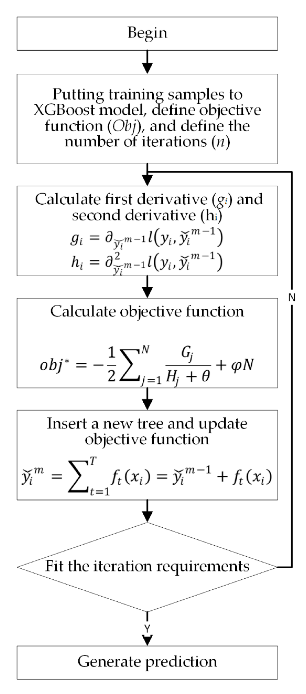
In recent years, some scholars have shown that the decision tree method can improve the accuracy of the TC intensity prediction. TC intensity in the western North Pacific was predicted using the decision tree method [17]. The theory and application of the decision tree method have developed significantly since Chen’s proposal of the eXtreme Gradient Boosting (XGBoost) model [18]; this model has been applied in several studies, on topics including image classification [19], speech recognition [20], and biomedical studies [21]. The XGBoost model has also proved to be useful in predicting TC intensity [22]. TC intensity is affected by several factors that are often ambiguous and uncertain. In this study, we used the XGBoost model to predict TC intensity, because its algorithm can handle many dimensions and be used to conduct multi-factor predictions. Factor mining has proved to be useful in forecasting model constructions [23,24]. The XGBoost model can also be used in conjunction with factor mining, which has proved to be useful in forecasting model construction. Furthermore, another advantage of the XGBoost model is its very low computational cost for users with a basic knowledge of TCs.

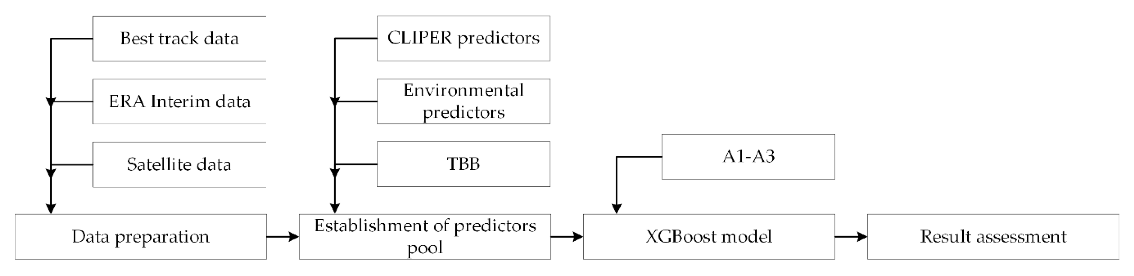
Therefore, we focused on using satellite predictors extracted via a new method, to establish a machine learning model for predicting TC intensity. This study aimed to establish an XGBoost-based framework to predict TC intensity in the South China Sea, using data from the China Meteorological Administration–Shanghai Typhoon Institute (CMA-STI) [25], meteorological variables from the European Centre for Medium-Range Weather Forecasts (ECMWF) [26], and satellite data from the National Satellite Meteorological Center FengYun Satellite Data Center, covering the period of 2006–2017. The differences between the predicted and observed data were used to analyze the dynamics of TC intensity development. The primary objectives of this study were: (1) to establish a South China Sea TC intensity prediction model based on the XGBoost framework and satellite-based potential predictors; (2) to analyze the influence of the FengYun-2 (FY-2) remote sensor data on TC intensity forecast results, and (3) to analyze the influence of the satellite data extraction method used on TC intensity forecast results.

2. Materials and Methods

We considered three types of potential predictors—satellite, best track, and environmental data—to establish a South China Sea TC intensity model, based on the framework shown in Figure 1. We prepared all the data and the theoretical basis for our models as described in Section 2.1 and Section 2.2. The formulation of the TC intensity prediction model is presented in Section 2.3.

2.1. Data

The South China Sea was chosen as the study area for three reasons. Firstly, TCs in the South China Sea include those generated locally and those that travel into the South China Sea from the western North Pacific Ocean [27]. Secondly, the accuracy of South China Sea TC track predictions in 2018 was significantly higher than that in 2017, but the accuracy of TC intensity predictions did not significantly improve in this time period [28]. Finally, several TCs with concentrated landing times have affected coastal areas of the South China Sea, and such storms may induce serious secondary disasters [29].

The datasets used in this study, including their spatial and temporal resolutions and temporal coverage, are described in

Table 1. Dataset characteristics.

Dataset		Spatial Resolution	Temporal Resolution	Spatial Coverage	Temporal Coverage
CMA-STI		0.1°	6 h	Northwest Pacific	1949–2017
ERA Interim		1° × 1°	6 h	Global	1979–2017
TBB	FY-2C	0.05° × 0.05°	1 h	Global	2006–2009
	FY-2E	0.05° × 0.05°	1 h	Global	2010–2017
	FY-2G	0.05° × 0.05°	1 h	Global	2015–2017

Note: TBB = blackbody temperature.

. Owing to the limitations of satellite data transmission time, the data used in this study relating to TCs and their surrounding environments in the South China Sea were limited to the period of 2006–2017. To ensure a well-constructed model, the ratio of training samples to experimental samples was approximately 7:3. TC data from 2006 to 2012 were selected for use as training samples and data from 2013 to 2017 were selected as the experimental samples. All TCs considered had been generated in or had entered the study area (105° E to 120° E, 10° N to 25° N) and had a minimum lifetime of 48 hours. The number of samples selected for each lead time is listed in

Table 2. Number of TC training and test samples used for 6, 12, 18, and 24 h lead-time assessments.

Lead Time (h)	All Samples (2006–2017)	Training Samples (2006–2012)	Test Samples (2013–2017)
6	1164	770	394
12	1041	697	344
18	922	625	297
24	808	557	251

.

The CMA-STI best track dataset includes the TC position (latitude and longitude), TC intensity category, minimum pressure near the TC center, and 2 min mean maximum sustained wind near the TC center. The 2006–2017 South China Sea TC datasets were downloaded from the CMA-STI best track dataset covering the western North Pacific (http://www.typhoon.gov.cn/) [25].

The environmental datasets were drawn from the ECMWF Re-Analysis (ERA-Interim) dataset [30]. This dataset provides assimilation analysis data four times daily at 00:00, 06:00, 12:00, and 18:00. Its spatial resolution is 1° × 1°. We selected environmental variables including relative humidity, temperature, divergence, and u- and v-wind at 200, 250, 300, 350, 400, 450, 500, 700, 750, 775, 800, 825, and 850 hPa. The maximum potential intensity (MPI) was estimated using sea surface temperature from the ERA-Interim dataset and CMA-STI best track dataset.

Remote sensing satellite data can provide high-precision meteorological information for TC intensity prediction [2]. In this study, satellite datasets were used to identify a convective intensity feature. The visible and infrared spin scan-radiometer sensor used on the CMA’s FY satellites is a scanning instrument that provides measurements of oceanic and atmospheric parameters relevant to regional water and energy cycles [31,32,33]. As different FY-series satellites operated during 2006–2017, data from the FY-2C, FY-2E, and FY-2G sensors were selected to cover the entire study period. The FY-2C satellite instrument was launched on October 19, 2004 and ceased operations on December 28, 2009, and the temporal coverage of the available data extended from May 2005 to January 2010. The FY-2E satellite instrument was launched on June 15, 2008 and ceased operations on June 2, 2015; the temporal coverage of the available data was from December 2009 to January 2019. The FY-2G satellite instrument was launched on June 3, 2015, and the temporal coverage of its available data extends from June 2015 to present. The FY-2 data obtained for this study were downloaded from the National Satellite Meteorological Center FengYun Satellite Data Center (http://satellite.nsmc.org.cn/PortalSite/Data/Satellite.aspx) [34]. The selected satellite product was the blackbody temperature (TBB), which represents the most primitive observational data for cloud formation and display enhancement.

2.2. Methods

2.2.1. XGBoost Theoretical Framework

The XGBoost model is a heavy end-to-end promoting tree system, that is improved based on a gradient-boosting decision tree algorithm [18]. XGBoost is an ensemble method that can integrate several weak learners into a powerful learner for prediction. XGBoost aims to prevent overfitting and decrease the cost of computing resources, by reducing the objective function using regularization terms. The prediction process using the XGBoost model is presented in Figure 2.

The XGBoost model generates a strong ensemble regression tree, through the combination of several weak regression trees. Firstly, according to the principles and requirements of the XGBoost model, we organized the training sample set, defined the objective function ($Obj$), and selected a number of iterations (n) for model training. Secondly, the first derivative $g_i={\partial }_{{\check{y_i}}^{m-1}}l\left(y_i,{\check{y_i}}^{m-1}\right)$ and second derivative $h_i={\partial }_{{\check{y_i}}^{m-1}}^{2}l\left(y_i,{\check{y_i}}^{m-1}\right)$ (calculated before the training) were summed, generating ($G_j$ and $H_j$). Thirdly, to prevent overfitting, we employed regularization and obtained a new objective function $ob{j}^{*}=-\frac{1}{2}{\displaystyle \sum }_{j=1}^N\frac{G_j}{H_j+\theta }+\phi N$. Fourth, we added a new tree to the original tree ${\check{y_i}}^m={\displaystyle \sum }_{t=1}^T{f}_t\left(x_i\right)={\check{y_i}}^{m-1}+f_t\left(x_i\right)$. After many iterations, the model’s ensemble regression trees were formed.

2.2.2. Embedded Selection Algorithm

Among the many predictors, predictor information is sometimes duplicated, and some predictors were not related to TC intensity. As inputting irrelevant predictors or predictors with repetitive information into the model reduces the model’s generalization ability, the embedded selection algorithm was used to select satellite predictors and remove irrelevant and duplicate predictors. Feature selection is automatically performed during the learning process of the algorithm, which can compensate for the shortcomings of the encapsulated and filtered feature selection algorithms. We used the learning model (XGBoost) to select the most valuable predictors for subsequent model design.

2.3. Formulation of the TC Intensity Prediction Model

A model for predicting the TC intensity in the South China Sea was established by applying XGBoost to FengYun satellite images. The predictor extraction and parameter adjustment methods employed in the TC intensity prediction model are discussed in Section 2.3.1 and Section 2.3.2, respectively, and our experimental design is presented in Section 2.3.3.

2.3.1. Predictor Extraction Method

This study aimed to develop a machine learning model for predicting TC intensity in the South China Sea, at lead times of 6, 12, 18, and 24 h. Climatology and persistence (CLIPER), environmental, and satellite-based predictors were used as input variables for the XGBoost model, and the output variable was TC intensity change.

Climatology and Persistence (CLIPER) Factors

Both linear and non-linear models have been built using CLIPER predictors to simulate TC intensity changes [35,36]. The CLIPER parameters values are computed in terms of TC location, pressure, and time of the year. To select relevant climatology and persistence factors, motion features and climatology and persistence factors at the initial time and during the previous period are described. The climatology and persistence variables used in this study were the same as those used by Baik [36] and Zhu [37], and because the month of occurrence of the TC and the intensity category of the TC affect the TC intensity, we added month and intensity categories based on the predictors proposed by Zhu [37]. The CLIPER predictors used in this study are given in

Table 3. Climatology and persistence, environmental, and satellite-based predictors used in this study.

Predictors	Description
Climatology and Persistence
Latitude	Latitude 0, 6, 12, 18, and 24 h ahead
Longitude	Longitude 0, 6, 12, 18, and 24 h ahead
Minimum pressure near the tropical cyclone (TC) center	Minimum pressure near the TC center 0, 6, 12, 18, and 24 h ahead
2 min mean maximum sustained wind near the TC center	2 min mean maximum sustained wind near the TC center 0, 6, 12, 18, and 24 h ahead
Month	Month of TC 0, 6, 12, 18, and 24 h ahead
Intensity category	TC intensity category 0, 6, 12, 18, and 24 h ahead
Environmental Factors
MPI	Maximum potential intensity based on equation (1) below
RHLO	Area-averaged (200–800 km) relative humidity at 700–850 hPa
RHHI	Area-averaged (200–800 km) relative humidity at 300–500 hPa
U200	Area-averaged (200–800 km) zonal wind at 200 hPa
T200	Area-averaged (0–1000 km) temperature at 200 hPa
D200	Area-averaged (200–800 km) divergence at 200 hPa
SHRS	Area-averaged (200–800 km) 500–850 hPa wind shear
SHRD	Area-averaged (200–800 km) 200–850 hPa wind shear
USHRS	Area-averaged (200–800 km) 500–850 hPa zonal wind shear
USHRD	Area-averaged (200–800 km) 200–850 hPa zonal wind shear
Vr850	Area-averaged (0–1000 km) 850 hPa relative vorticity
Satellite-based Factors
TBB	Equivalent blackbody temperature

. Following this preliminary selection, a set of potential CLIPER predictors for TC intensity at each lead time (6, 12, 18, and 24 h) was chosen. To fully show the effects of the CLIPER predictors, we established square terms based on the existing CLIPER factors. In addition to the predictors in Table 3, other potential predictors are described in Jin [22].

Environmental Factors

Table 3 also presents the environmental variables used in the study. Environmental factors were obtained according to the “perfect prog” theory [8,38]. Perfect prog is an ideal application environment, which generally uses a multiple linear regression model to process the output of a numerical model, which in this case is the predictors. In the experimental stage, we use reanalysis data to replace the output of the numerical model. The environmental factors selected in this study were divided into three categories, including factors related to sea surface temperature, moisture fields, and wind fields. The values for the first category were drawn from the ERA-Interim dataset and were interpolated into the TC center, and those for the latter two categories were averaged around the center.

Sea surface temperature (SST) primarily serves to estimate the upper bound of TC intensity. The best indicator to describe the upper bound of TC intensity is MPI. MPI values can be calculated theoretically [39,40,41] or empirically [8,39,42]. The empirical method was selected based on the approach of DeMaria and Kaplan [39]. The SST selected from the ERA-Interim dataset was interpolated to the TC center according to the best track data from 2006–2017, to determine the relationship between SST and TC intensity [9], as follows:

$$\mathrm{MPI}=\mathrm{A}+\mathrm{B}{e}^{C\left(T-T_0\right)}$$

(1)

The values were set as follows: A = 17.76 m/s, B = 49.69 m/s, C = 0.1218 °C⁻¹, and $T_0$ = 30.0 °C. The maximum value of MPI was 75 m/s. The CMA-STI best track dataset and 2 min sustained maximum wind speed were used to compute the correlation coefficient in our study, whereas Knaff used the JTWC best track dataset and 1 min sustained maximum wind speed to estimate the coefficient.

Because convection is the direct power source for a TC, variations in relative humidity can affect the TC intensity [9]. The average relative humidity at 700, 750, 800, and 850 hPa (RHLO); average relative humidity at 300, 400, 450, and 500 hPa (RHHI); zonal wind at 200 hPa (U200); temperature at 200 hPa (T200); divergence at 200 hPa (D200); relative vorticity at 850 hPa (Vr850); average zonal wind shear at 500, 700, 750, 800, and 850 hPa (USHRS); and average wind shear at 200, 250, 300, 400, 450, 500, 700, 750, 800, and 850 hPa (USHRD) were chosen as the environmental predictors to assess the potential impact of moisture and wind fields on TC intensity. As vertical wind shear has also been found to be crucial in predicting TC intensity [9,36,43], we considered two additional factors, defined as the difference between the 850 and 200 hPa horizontal wind vectors (SHRS) and the difference between the 850 and 500 hPa horizontal wind vectors (SHRD). We applied an environmental factor extraction method, based on the approach of Gao and Knaff [8,9,44]. To fully show the effects of environmental factors, we established some square and cubic terms based on the existing factors [8,9]. In addition to the predictors in Table 3, other potential predictors are described in Jin [22].

Satellite-Based Factors

The relationship between TBB and TC intensity has previously been quantified [45,46,47]. Weatherford and Gray [48] showed that TCs have fast outer-core winds that restrict inflow to the eye-wall; based on their results, Mundell [49] noted that a high ratio of inner-to outer-core convection indicates future intensification, as this suggest that the inner-core processes dominate over outer-core processes. Based on these findings, Fitzpatrick [47] showed in a study of TBB ranges from 0–6° in intervals of 1° that TBB data contain additional important convection information. Chen [45] applied predictors, including max, min, and mean TBB, within spatial regions to predict TC intensity. Chen’s findings regarding TBB, however, applied characteristics identified in earlier literature and produced no uniform law. To extract TBB features more precisely and accurately, we designated a spatial region based on a correlation coefficient. The 0.05° × 0.05° resolution of the FengYun satellite data used in this study is quite different from those used in previous studies and offers more detailed TBB information.

We analyzed the correlation between the satellite data and TC intensity. In Figure 3a, which shows the correlation coefficients (CCs) between TC intensity and TBB, there is a negative correlation in most areas; in other words, a lower TBB indicates stronger convection. Figure 3b–e show the maximum CCs between contemporary TBB data in the region and TC intensities at 6, 12, 18, and 24 h lead times, which were −0.56, −0.52, −0.47, and −0.41, respectively. The CCs between the TBB of the TC center and the TC intensity became smaller with longer lead times. Figure 3b–e show significantly negative correlations in areas spreading to the west as the lead time extended. The most important part of each figure is its center, corresponding to the clearly visible eye of the TC, at which the absolute value of the CC was less than the absolute value of the CC in the surrounding areas. This phenomenon suggests that the CC in the eye decreases with longer lead times. TBB data obtained from IR (infrared radiation) imagery contain important information regarding TC intensity. The figures show that negative correlations occurred at approximately 4° around each TC center, which was used to determine the TBB selection area radius of 4° in the next step.

We then extracted satellite-based predictors from the TBB images in Figure 4. Fitzpatrick [47] established radial areas of 0–1°, 0–2°, 0–4°, 0–6°, 1–2°, 2–4°, and 2–6°, with TBBs ranging from 193–218 K in 5 K increments. An examination of Figure 3 reveals that negative correlations were primarily distributed at 4° around the TC center. In our adaptation of Fitzpatrick’s methods, we processed radial annuli over 0–4°from the TC center in 0.1° increments. The corresponding TBB measurements were extracted from each of the 40 annuli. This approach allowed us to extract information regarding the TC in greater detail and to address the phenomenon of TC convection.

Table 4. Satellite-based predictors.

Predictors	Description
GAP0201_N	Number of infrared pixels in a radial area colder than 218 K at the N annuli band.
GAP0202_N	Number of infrared pixels in a radial area colder than 213 K at the N annuli band.
GAP0203_N	Number of infrared pixels in a radial area colder than 208 K at the N annuli band.
GAP0204_N	Number of infrared pixels in a radial area colder than 203 K at the N annuli band.
GAP0205_N	Number of infrared pixels in a radial area colder than 198 K at the N annuli band.
GAP0206_N	Number of infrared pixels in a radial area colder than 193 K at the N annuli band.
GAP02max_N	Max value of TBB in a radial area at the N annuli band.
GAP02maxc_N	Difference between the center TBB value and the max TBB within a radial area at the N annuli band.
GAP02mean_N	Mean TBB in a radial area at the N annuli band.
GAP02min_N	Min value of TBB in a radial area at the N annuli band.
GAP02minc_N	Difference between the center TBB value and the min TBB within a radial area at the N annuli band.
GAP02stand_N	Standard deviation TBB in a radial area at the N annuli band.

presents descriptions of the TBB-extracted factors. GAPRxTb_N represents the number of pixels in each radial area colder than a specified TBB, where Rx indicates the radial increment, Tb indicates the TBB value (193 K, 198 K, 203 K, 208 K, 213 K, and 218 K), and N indicates the location of rings. For example, the number of pixels in a 0–0.1° radial area that were colder than 193 K are denoted as GAP0206_1, and the number of pixels in a 2–2.1° radial area that were colder than 208 K are denoted GAP0206_21. GAP02max_N indicates the maximum TBB in each spatial area; for example, the maximum TBB in a 0–0.1° radial area is designated GAP02max_1. GAP02min_N indicates the minimum TBB in each radial area; for example, the minimum TBB in a 0–0.1° radial area is termed GAP02min_1. Similarly, GAP02mean_N indicates the mean TBB in each radial area; for example, the mean TBB in a 0–0.1° radial area is designated as GAP02mean_1. Finally, the differences between the TBB value of the center and the maximum and minimum values are designated as GAP02maxc_N and GAP02minc_N, respectively.

2.3.2. Parameters for Adjusting the TC Intensity Prediction Model

The resulting XGBoost model contained many important parameters that required adjustments to fit different scenarios. These included the eta parameter, which was designed to reduce the individual feature weights, avoid overfitting, and apply shrinkage steps in process updates; the gamma parameter, which was used to further partition the tree leaf nodes to reduce losses; the max_depth parameter representing the maximum depth of a tree; and the min_child_weight parameter, representing the minimum weight coefficient of the leaf nodes. We selected the best parameters for a 6 h lead time prediction model, corresponding to the eta, gamma, max_depth, and min_child_weight values of 0.1, 0.8, 8, and 4, respectively; the best parameters for 12 and 18 h lead times were determined to be eta, gamma, max_depth, and min_child_weight values of 0.1, 0.8, 6, and 4, respectively; and the best parameters for a 24 h lead time were found to be eta, gamma, max_depth, and min_child_weight values of 0.1, 0.8, 6, and 2, respectively.

2.3.3. Experiment

Table 5. Input and output parameters of the three prediction models.

Model	Input Parameters	Type	Output Parameters
A1	CLIPER + environmental predictors	XGBoost	TC intensity (t + ∆t) ∆t = 6, 12, 18, and 24 h, respectively.
A2	A1 + S_mean
A3	A1 + S_2

lists input and output parameters of the three models evaluated in the study. The input parameters include, CLIPER factors, environmental predictors, and satellite-based predictors. To assess various extraction methods for satellite-based predictors, we designed two methods to extract satellite-based predictors from brightness temperature images.

The first model, A1, served as a control in which CLIPER and environmental predictors were used as input parameters. The second model (A2) was developed using the XGBoost model based on the input parameters of the A1 model plus the satellite-based predictors. The average satellite-based predictor values (abbreviated as S_mean) were calculated within a range of 4° from the TC center. The satellite-based predictors were extracted via the traditional method widely used in the SHIPS model [7]. The third model (A3) was also developed using the XGBoost model, based on the input parameters of the A1 model plus the satellite-based predictors. However, the extraction method for the satellite-based predictors divided each image into 40 annuli bands of 2 pixels each around the TC center. For each band, the mean, standard deviation, minimum, maximum, difference between the center TBB value and the max TBB within a radial area, difference between the center TBB value and the min TBB within a radial area, number of infrared pixels in a radial area colder than 218 K, number of infrared pixels in a radial area colder than 213 K, number of infrared pixels in a radial area colder than 208 K, number of infrared pixels in a radial area colder than 203 K, number of infrared pixels in a radial area colder than 198 K, and number of infrared pixels in a radial area colder than 193 K, were calculated. Using this method, referred to as the “ring segmentation method” (S_2), 480 (12 × 40) predictors were extracted.

As shown in Table 5, each of these models contained different input parameters. The output parameter was TC intensity at 6, 12, 18, and 24 h. In this study, the TC samples from 2006–2012 were used for model training, and the remaining samples, from 2013–2017, were used for verification.

To evaluate the performance of each XGBoost model corresponding to a given lead time during the training and validation periods, we used the CC (correlation coefficient), mean absolute error (MAE), and normalized root mean square error (NRMSE).

3. Results

3.1. Feature Selection

To verify the relationship between the statistical information extracted from 40 circular bands and the TC intensity, a scatter plot of the satellite predictors and the TC intensity was generated using the correlation coefficient, as shown in Figure 5. The results showed that the number of pixels colder than 218, 213, 208, 203, 198, and 193 K in each ring had a positive correlation with TC intensity. As distance from the TC center increased, the correlation coefficient first increased and then decreased, indicating that the number of pixels colder than 218, 213, 208, 203, 198, and 193 K in each ring was indicative of the TC intensity. The maximum brightness temperature value in each ring had a negative correlation with the TC intensity. As the distance from the TC center increased, the correlation coefficient of brightness temperature and TC intensity first increased and then decreased, indicating that the maximum brightness temperature value in each ring could indicate the strength of the relationship with TC intensity.

The TBB information was fully extracted via the ring segmentation method, and 480 satellite predictors were obtained. However, among these 480 predictors, some predictor information was duplicated, or was not related to TC intensity. To properly control the number of selected factors, 10 prediction factors were selected as the model input based on the feature ranking of the learning model. The filtered information gain ranking results are shown in

Table 6. Selected satellite factors at lead times of 6, 12, 18, and 24 h.

	Time	6 h	12 h	18 h	24 h
No.
1		GAP02max_13	GAP02max_12	GAP0203_8	GAP0201_7
2		GAP02max_11	GAP02max_13	GAP02max_12	GAP0203_8
3		GAP0203_8	GAP02max_11	GAP02max_13	GAP02max_18
4		GAP02max_14	GAP0203_8	GAP02max_16	GAP0201_10
5		GAP0201_6	GAP02max_16	GAP0201_8	GAP02max_13
6		GAP02max_15	GAP0202_6	GAP0202_8	GAP02max_16
7		GAP0201_8	GAP0203_10	GAP02max_11	GAP0201_6
8		GAP0202_6	GAP02stand_2	GAP0204_10	GAP0201_8
9		GAP02max_12	GAP0203_7	GAP0202_6	GAP02max_11
10		GAP02max_17	GAP02max_15	GAP02stand_1	GAP02max_14

. The smaller the serial number, the higher the correlation between the predictor and the prediction result. The sorting results indicate that different satellite predictors were best suited for TC intensity prediction models with different lead times. The following main findings were found: (1) for a 6 h lead time, the selected satellite-based predictors included the maximum TBB in the 1.0–1.5° radial area, the maximum TBB in the 1.6–1.7° radial area, the pixels colder than 218 K at radii of 0.5–0.6° and 0.7–0.8°, the pixels at radii of 0.5–0.6° colder than 213 K, and the pixels at radii of 0.7–0.8° colder than 208 K; (2) for a 12 h lead time, the selected satellite predictors included the maximum TBB in the 1.0–1.3° radial area, the maximum TBB in the 1.4–1.6° radial area, the pixels colder than 213 K at radii of 0.5–0.6°, and the pixels colder than 208 K at radii of 0.7–1.0°; (3) for an 18 h lead time, the selected satellite predictors included the maximum TBB in the 1.0–1.3° radial area, the maximum TBB in the 1.5–1.6° radial area, the pixels colder than 218 K at radii of 0.7–0.8°, the pixels colder than 213 K at radii of 0.5–0.6° and 0.7–0.8°, the pixels colder than 208 K at radii of 0.7–0.8°, and the pixels colder than 203 K at radii of 0.9–1.0°; (4) for a 24 h lead time, the selected satellite predictors included the maximum TBB in the 1.0–1.1°, 1.2–1.4°, 1.5–1.6°, and 1.7–1.8° radial areas, the pixels colder than 218 K at radii of 0.6–0.8° and 0.9–1.0°, and the pixels colder than 208 K at radii of 0.7–0.8°. No good predictors were found outside of the first 20 rings (2.0°) and within the first five rings (0.5°); this supports the analysis utilized in other objective schemes such as the Advanced Dvorak Technique [50]. The aforementioned finding suggests that most of the information regarding TC intensity that can be obtained using IR imagery is within the inner core region, and this indicates that once the eye appears, less relevant information is available for TC intensity prediction. Thus, the selected satellite parameters were located in rings 6–17 (0.5–1.7° from the TC center) and included the number of pixels in these rings that were colder than 218, 213, 208, and 203 K.

3.2. TC intensity Prediction Accuracy

After the three types of predictors had been processed, the TC intensity prediction model was run. This section describes the training results of each model. The results concerning the test samples in the XGBoost model are introduced first, and then the prediction results for each lead time are presented.

TC intensity information from the South China Sea from 2006 to 2012 was used as training data for models A1, A2, and A3, and the TC intensity from 2013 to 2017 was predicted and verified.

Table 7. Errors of the TC intensity at 6, 12, 18, and 24 h lead times.

Lead Time	Models	Accuracy
		MAE	NRMSE	CC
6 h	A1	2.20	5.68	0.94
	A2	2.15	5.40	0.94
	A3	2.14	5.28	0.95
12 h	A1	3.56	9.19	0.82
	A2	3.35	8.33	0.86
	A3	3.29	8.19	0.87
18 h	A1	4.45	10.69	0.75
	A2	4.19	9.58	0.81
	A3	4.11	9.42	0.82
24 h	A1	4.96	11.33	0.69
	A2	4.96	10.80	0.73
	A3	4.71	10.51	0.75

Note: MAE: mean absolute error; NRMSE: normalized root mean square error; CC: correlation coefficient.

shows the TC intensity results (CCs, MAE, and NRMSE) for 6, 12, 18, and 24 h lead times. The best model for each lead time is indicated in bold. The A3 model (A1 + S_2) and A2 model (A1 + S_mean) produced better forecasts than the A1 model. Among the models, A3 had the lowest MAE and NRMSE values and the highest CC values. For all lead times, the MAE of model A3 was lower than that of both A1 and A2. These results indicate that the forecast skills of models A3 and A2, with their satellite-based predictors, were better than those of A1, which did not use satellite-based predictors. As shown in the table, as lead times increased, the MAE and NRMSE values became larger and the CC values became smaller. For example, in the A2 model at 6, 12, 18, and 24 h lead times, the MAE values were 2.15 m/s, 3.35 m/s, 4.19 m/s, and 4.96 m/s, and the CC values were 0.94, 0.86, 0.81, and 0.73, respectively. The NRMSE values were 5.40, 8.33, 9.58, and 10.80. The 6 h CC for model A3 was 0.95, and its 6 h MAE was 2.14 m/s. Its 6 h NRMSE was 5.28% lower than that of model A2. The 12 h CC for model A3 was approximately 0.87. The 12 h MAE for model A3 was 3.29 m/s lower than that of model A1. The 18 h CC for model A3 was approximately 0.82. The 24 h MAE for model A3 was approximately 4.71 m/s, and A3 produced the lowest MAE value for a 24 h lead time. These results suggest that the combination of predictors in A3 is well suited to forecasting TC intensity at lead times of 6, 12, 18, and 24 h. For each model, the CC values decreased with time, while the MAE and NRMSE values both increased. The CCs of model A3 were approximately 0.95, 0.87, 0.82, and 0.75 at lead times of 6, 12, 18, and 24 h, respectively. The MAEs of all models ranged from 2.14 to 2.20 m/s, 3.29 to 3.56 m/s, 4.11 to 4.45 m/s, and 4.71 to 4.96 m/s, at lead times of 6 12, 18, and 24 h, respectively. The NRMSEs of all models ranged from 5.28 to 5.68 m/s, 8.19 to 9.19 m/s, 9.42 to 10.69 m/s, and 10.51 to 11.33 m/s at lead times of 6 12, 18, and 24 h, respectively.

3.3. Comparison of the Different Models

Figure 6 (A1_6, A2_6, and A3_6) shows scatterplots of the intensity predictions produced by the three models and the actual intensity values at 6, 12, 18, and 24 h lead times. The overall model fit between the predicted values of model A1 and the actual values was fairly strong with a R² of 0.88, indicating that the model had a good ability to predict TC intensity. Model A2 added averaged satellite data to the predictors considered by model A1, and its R² and relative bias were slightly improved over that of the first model. Compared with model A1, the R² and relative bias of model A3 increased to 0.91 and the relative bias of model A3 decreased to 8.62%. The results show that the prediction ability of model A3 with a 6 h lead time was considerably better than those of models A1 and A2.

Figure 6 (A1_12, A2_12, and A3_12) shows scatterplots of the intensities predicted by the models at a 12 h lead time and the actual intensity values. The overall model fit between model A1’s predicted values and the actual values was fairly good, with a R² of 0.73. Model A2’s R² was 0.74, representing a slight improvement over that of A1. The R² of model A3 improved to 0.82. The relative bias of model A3 decreased to 12.57%. In the figure, the fitting line of model A3 is closer to that of the actual values (the red line), than those of models A1 and A2. These results show that the prediction ability of model A3 at a 12 h lead time is significantly better than that of models A1 and A2.

Figure 6 (A1_18, A2_18, and A3_18) shows scatterplots of the predicted intensity values of the three models with an 18 h lead time and the actual values. Model A1 achieved a R² of 0.61, which shows that the model had a good ability to predict TC intensity. Model A2’s R² improved slightly to 0.66, while A3’s R² increased to 0.73. Model A2’s relative bias decreased slightly to 17.96%, while A3’s relative bias decreased to 16.48%. The fitting line of model A3 was near that of the actual values (the red line) than were those of models A1 and A2. Thus, model A3 had a significantly better predictive ability than that of models A1 and A2 at an 18 h lead time.

Finally, Figure 6 (A1_24, A2_24, and A3_24) shows scatterplots of the predicted and actual intensity values at a 24 h lead time. A1 achieved a R² of only 0.51, indicating a poor ability to predict TC intensity. Model A2’s R² was slightly improved, at 0.56, and that of model A3 increased to 0.63. Model A2’s relative bias was slightly decreased, at 21.93%, and that of model A3 decreased to 19.04%. The fitting line of model A3 was closer to that of the actual values (red line) than were those of models A1 and A2. The results demonstrate that the predictive ability of model A3 at a 24 h lead time is significantly better than that of models A1 and A2.

Table 8. Comparative analysis of TC intensity prediction at 6, 12, 18, and 24 h lead times.

Lead Time	Model	Relative Bias (%)	R2
6 h	A1	9.58	0.88
	A2	9.22	0.88
	A3	8.62	0.91
12 h	A1	14.88	0.73
	A2	13.76	0.74
	A3	12.57	0.82
18 h	A1	20.99	0.61
	A2	17.96	0.66
	A3	16.48	0.73
24 h	A1	23.94	0.51
	A2	21.93	0.56
	A3	19.04	0.63

presents further comparison of the accuracy of the three models, including relative bias and R² values. In each case, A3 was found to offer the best perform for TC intensity prediction.

3.4. Forecast Skill at Different Intensities

3.4.1. Long Short-Term Memory (LSTM) Model

The long short-term memory (LSTM) model introduces an input gate, output gate and forgetting gate in each neuron of a recurrent neural network, to describe and predict the long-term dependence of time series data [51]. The model has been applied in many fields, such as tropical cyclone path prediction [52], traffic volume prediction [53], and future land-use prediction [54], demonstrating its popularity as a time series-based prediction model.

Figure 7 shows the structure of the LSTM model. The main components of the model include the input gate ($i_t$), output gate ($o_t$), update gate ($i{m}_t$), forget gate ($f_t$), cell memory ($C_t$), and cell output ($h_t$).

$W^i$, $W^f$, $W^{im}$, and $W^o$ represent the weight of the input gate, forget gate, update gate, and output gate, respectively. $b^{\left(i\right)}$, $b^{\left(f\right)}$, $b^{\left(im\right)}$, and $b^{\left(o\right)}$ represent the bias of the input gate, forget gate, update gate, and output gate, respectively. $\sigma$ represents sigmoid activation, and $tanh$ represents hyperbolic tangent activation. The main operative processes of the model are as follows:

$$f_t=\sigma \left(W^f·\left[h_{t-1},x_t\right]+b^{\left(f\right)}\right)$$

(2)

$$i_t=\sigma \left(W^i·\left[h_{t-1},x_t\right]+b^{\left(i\right)}\right)$$

(3)

$$i{m}_t=tanh\left(W^{im}·\left[h_{t-1},x_t\right]+b^{\left(im\right)}\right)$$

(4)

$$C_t=i_t·i{m}_t+f_t·C_{t-1}$$

(5)

$$o_t=\sigma \left(W^o·\left[h_{t-1},x_t\right]+b^{\left(o\right)}\right)$$

(6)

$$h_t=o_t·\tan \mathrm{h}\left(C_t\right)$$

(7)

where “·” represents the point multiplication operation of two vectors.

3.4.2. Comparative Analysis

To further study the prediction performance of model A3, we used the LSTM model to predict the intensity of TCs in the South China Sea, using the same predictors (hereafter referred to as the LSTM-TCIPS; model A3 will hereafter be referred to as XGB-TCIPS). As these two models yielded different results for TCs with different intensities, the TC intensities recorded in the South China Sea in 2013–2017 were used to analyze the models’ predictive abilities according to different TC intensity types at 6, 12, 18, and 24 h lead times.

Table 9. LSTM and XGBoost model errors for different tropical cyclone intensity levels at a 6 h lead time.

Type	LSTM		XGBoost
	MAE (m/s)	NRMSE	MAE (m/s)	NRMSE
Tropical depression	1.56	3.10	1.45	2.9
Tropical storm	2.07	4.05	1.89	4.21
Severe tropical storm	3.48	6.62	2.34	5.49
Typhoon	6.91	12.19	2.99	5.87
Severe typhoon	12.23	20.49	2.74	5.36
Super typhoon	19.77	32.73	13.91	24.6

Note: LSTM: long short-term memory; MAE: mean absolute error; NRMSE: normalized root mean square error.

,

Table 10. LSTM and XGBoost model errors for different tropical cyclone intensity levels at a 12 h lead time.

Type	LSTM		XGBoost
	MAE (m/s)	NRMSE	MAE (m/s)	NRMSE
Tropical depression	2.55	6.17	2.17	5.46
Tropical storm	2.72	5.65	2.66	6.14
Severe tropical storm	4.25	8.03	3.69	7.81
Typhoon	5.14	10.51	4.01	7.81
Severe typhoon	9.78	18.44	6.35	12.43
Super typhoon	18.12	31.03	20.15	34.66

Note: LSTM: long short-term memory; MAE: mean absolute error; NRMSE: normalized root mean square error.

,

Table 11. LSTM and XGBoost model errors for different tropical cyclone intensity levels at an 18 h lead time.

Type	LSTM		XGBoost
	MAE (m/s)	NRMSE	MAE (m/s)	NRMSE
Tropical depression	3.44	8.29	3.11	7.43
Tropical storm	3.22	6.67	3.42	7.31
Severe tropical storm	4.74	9.23	4.24	8.12
Typhoon	6.33	12.85	4.17	8.41
Severe typhoon	12.03	22.65	9.50	16.79
Super typhoon	21.69	36.12	21.20	35.39

Note: LSTM: long short-term memory; MAE: mean absolute error; NRMSE: normalized root mean square error.

and

Table 12. LSTM and XGBoost model errors for different tropical cyclone intensity levels at a 24 h lead time.

Type	LSTM		XGBoost
	MAE (m/s)	NRMSE	MAE (m/s)	NRMSE
Tropical depression	4.79	10.61	3.9	8.94
Tropical storm	3.67	7.47	3.82	7.95
Severe tropical storm	4.51	8.37	4.52	8.78
Typhoon	6.66	14.19	5.15	10.58
Severe typhoon	13.07	24.25	10.55	18.34
Super typhoon	22.04	36.24	22.61	37.86

Note: LSTM: long short-term memory; MAE: mean absolute error; NRMSE: normalized root mean square error.

compare the performances of the two models. It was found that at increased lead times, the LSTM-TCIPS model is more suitable for forecasting higher intensity levels, indicating that this model is more suitable for longer-term TC prediction, whereas the XGB-TCIPS model is better suited for short-term predictions. These conclusions were based on the following: (1) at a 6 h lead time, the XGB-TCIPS model had a smaller average absolute error than did the LSTM-TCIPS model for TCs of all intensity levels, and the XGB-TCIPS model was suitable for all intensity types. (2) At a 12 h lead time, the XGB-TCIPS model was more suitable for the prediction of tropical depressions, severe tropical storms, typhoons, and strong typhoons, whereas the LSTM-TCIPS model was better suited for the prediction of super typhoons. (3) At an 18 h lead time, the XGB-TCIPS model was better suited for the prediction of tropical depressions, severe tropical storms, typhoons, strong typhoons, and super typhoons, whereas LSTM-TCIPS was better suited for the prediction of tropical storms. (4) For a 24 h lead time, the XGB-TCIPS model was more suitable for the prediction of tropical depressions, typhoons, and strong typhoons, and the LSTM-TCIPS model was better suited for the prediction of tropical storms, severe tropical storms, and super typhoons.

4. Discussion

In this study, we developed a new TC intensity prediction model that is based on the XGBoost model; the proposed model integrates climatology and persistence, environmental, and satellite-based predictors. Climatology and persistence factors can provide a more detailed description of TC motion features. Environmental factors can reflect the synoptic features of TC in the South China Sea. The TBB features are used to characterize the structure and the development of convection. Our experimental results demonstrate that satellite data can improve the accuracy of TC intensity prediction, particularly when TBB is used as input data. The MAE of model A2, which included S_mean satellite predictors that were not considered in A1, produced improvements of 2.27%, 5.90%, 5.84%, and 0.00% over the MAEs of A1 at lead times of 6, 12, 18, and 24 h. However, the MAE of model A3, which includes satellite predictors extracted via method S_2, produced MAE improvements of 2.73%, 7.58%, 7.64%, and 5.04% for lead times of 6, 12, 18, and 24 h over those of model A1. The conclusions of model A3 were also consistent with those of STIPER (Statistical Typhoon Intensity Prediction including surface Evaporation and inner core Rainfall) [9].

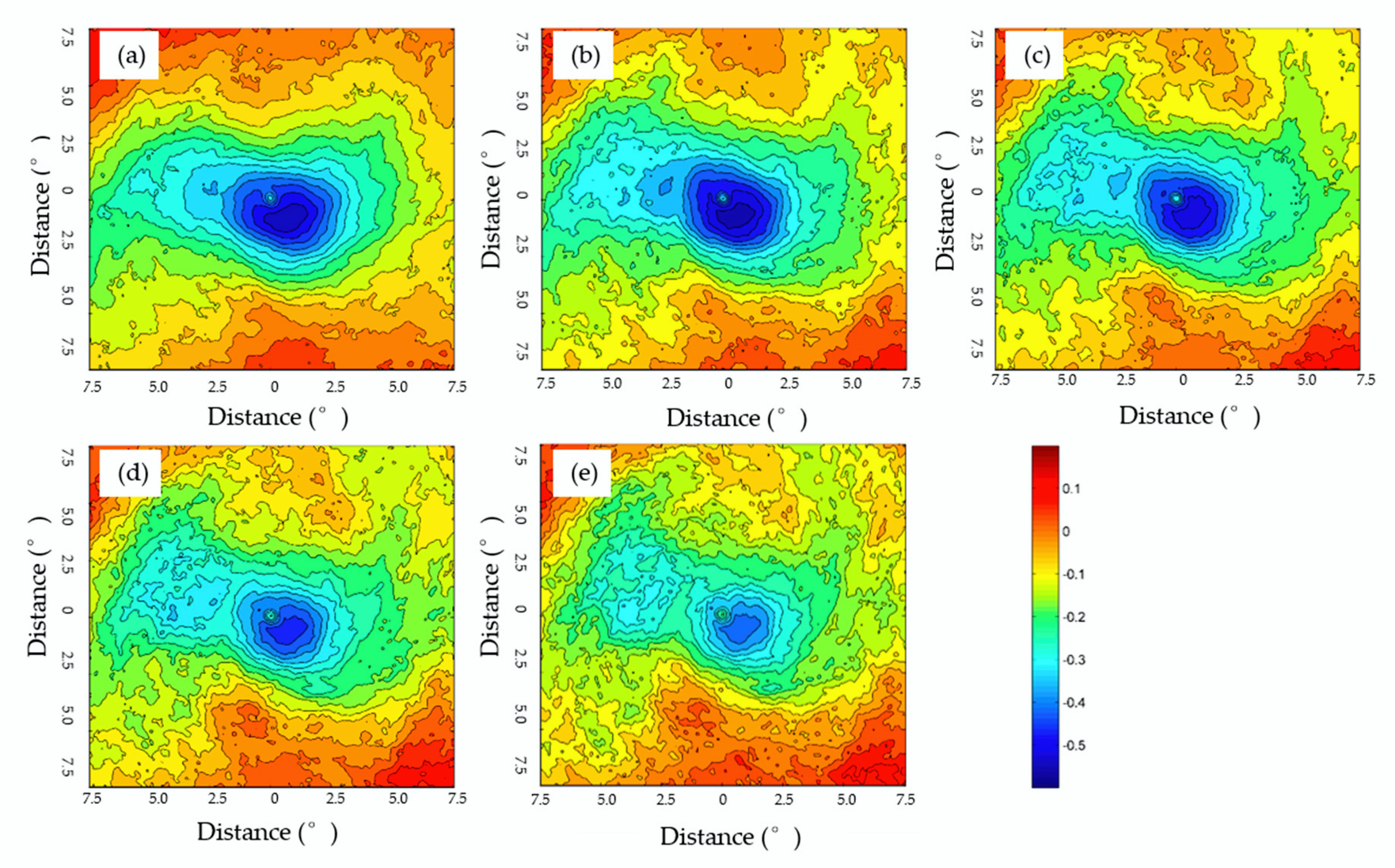
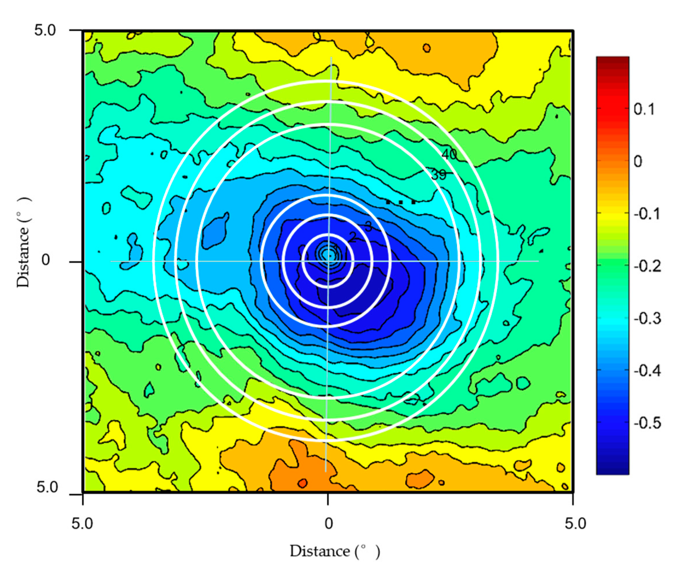
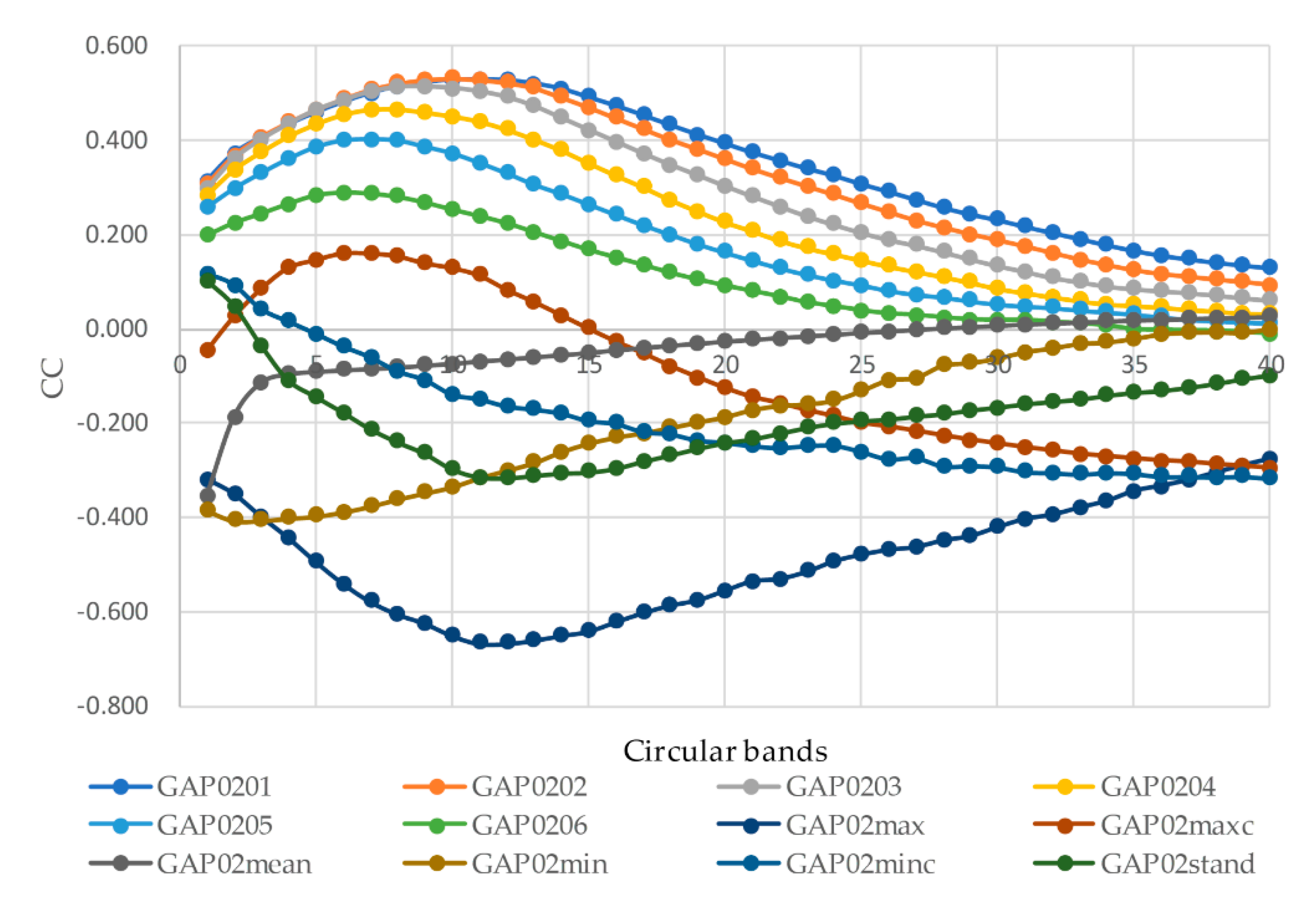
In this study, we developed a new extraction method (the “ring segmentation method”) for satellite image data. Our experimental results suggested that the ring segmentation method can improve the accuracy of TC intensity prediction. The MAE of model A3 (A1 + satellite-based predictors extracted via ring segmentation) decreased by 0.47%, 1.79%, 1.91%, and 5.04% at 6, 12, 18, and 24 h lead times, respectively, compared to those of model A2 (A1 + satellite-based predictors extracted as mean values). There are two possible reasons for this. The first is that high-resolution FY satellite data can provide detailed information on TC structure. For example, we noted that the TC intensity attributes extracted from TBB features in FY-2 images included the TC cloud-top convection strength, distribution, and size, all of which are closely related to TC intensity. The absolute CC values between the TBB values at the TC centers and the TC intensity become smaller at longer lead times. Muramatsu [55] suggested that TBB has a very high correlation with TC intensity and is therefore very important in TC prediction. High-resolution FY-2 satellite data allow TBB_C data to be extracted at smaller intervals (0.1°), allowing us to obtain 480 features from the TBB images by applying Fitzpatrick’s extraction method [47]. The factors related to TC intensity at lead times of 6, 12, 18, and 24 h were extracted using the ring segmentation method, and the small intervals at which these data could be extracted provided detailed descriptions of the relationships between the TBB and TC intensity. The pixels colder than a particular TBB at given radii were also helpful in improving TC intensity prediction. Pixels colder than 253.15 K at a radius of 2° were found to be a noteworthy predictor of intensity [56]. At a 24 h lead time, the highest predictive value was found for pixels colder than 218 K at radii of 0.6–0.7°. Pixels colder than 208 K represent a deep convective region [57]. At an 18 h lead time, the number of pixels colder than 208 K at radii of 0.7–0.8° was the most significant predictor of TC intensity, indicating that deep convection regions are also very important for predicting TC intensity at lead times close to 18 h. In another study, the highest correlation between the maximum TBB and TB intensity was found in the 1.4° radial area at a 0–36 h lead time [45]. In this study, the highest correlation between TBB and TC intensity was found in the 1.1–1.5° radial area at a 6–12 h lead time. Because our extraction method allowed us to employ high-resolution FY-2 satellite data, our results can be considered more precise than those found in previous studies.

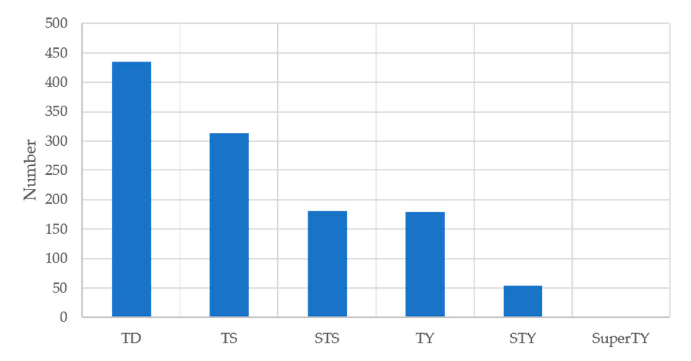
The second reason that the ring segmentation method led to better results is that the XGBoost model allows multi-predictor input. In this study, we assessed the response of the model to different combinations of input features related to TC intensity in the South China Sea, such as inner-core convection, climatology and persistence factors, and environmental factors. The resulting combination of predictors obtained from the TBB features derived from the FY-2 satellite data, the best track data taken from the CMA-STI, and environmental information obtained from the ERA-Interim dataset were then used to build the final model. Because the model primarily uses randomly selected features, each tree can be built from a random set of features rather than the overall set. Combining all trees constructed in this manner led to the most accurate predictions. In this study, we used approximately 100 predictors that did not produce any serious over-fitting in the XGBoost model, because an appropriate scale was used to select the eta hyperparameters. However, we did identify one limitation in our proposed model. Its errors when predicting the intensity of very strong storms in the “severe typhoon” and “super typhoon” intensity categories were substantially large at lead times of 6, 12, 18, 24 h. This limitation is likely attributable to the relatively low number of samples concerning high-intensity TC events, leading to larger model errors concerning these types of storms. Figure 8 shows the frequencies of different TC intensities in the South China Sea from 2006 to 2012. Cyclones in the severe typhoon and super typhoon categories have the lowest occurrence in the training data. Owing to the lack of training samples, the accuracy of the model, with regard to severe typhoons and super typhoons, is low.

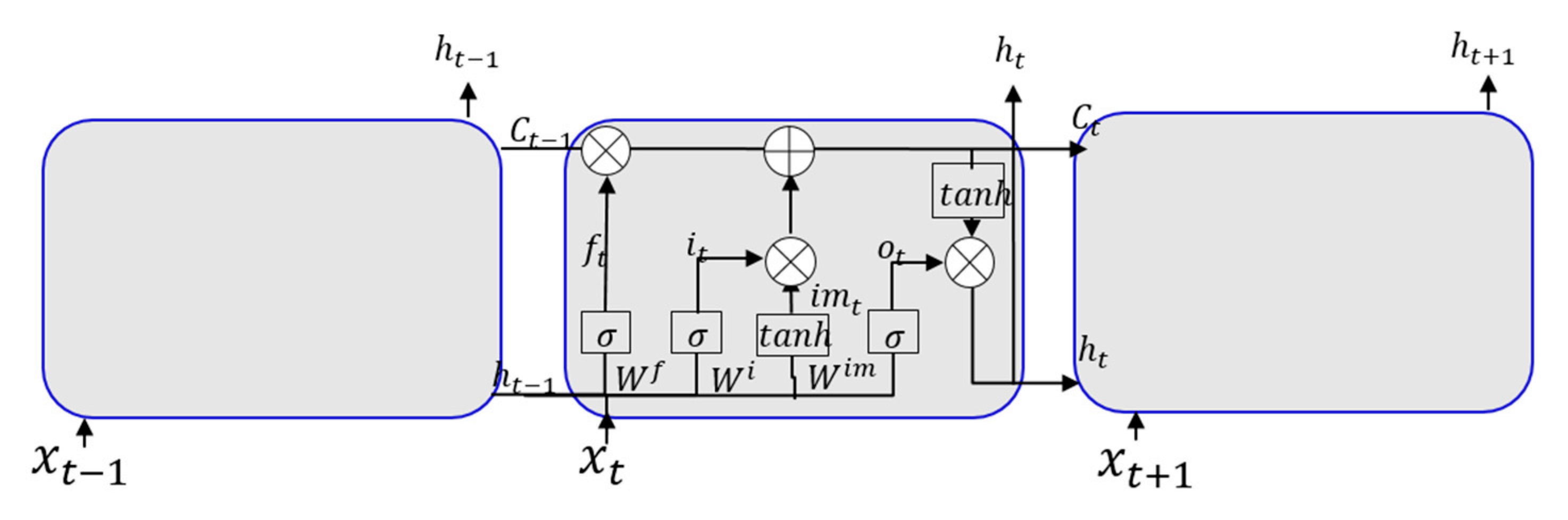
The XGBoost method and the LSTM method can both predict TC intensity from a non-linear perspective. The XGBoost method essentially incorporates the XGBoost algorithm into the TC intensity prediction model, which improves the average absolute error of the existing TC intensity model predictions. The combination of feature selection and the spatio-temporal consideration of the LSTM model can also improve TC intensity predictions. The performance of each of the models seems to be dependent on lead time; the XGBoost model is best applied to the prediction of TC intensity at short lead times. At a 6 h lead time, the MAE and NRMSE values obtained using the XGBoost model were better than those of the LSTM model, for storms of all intensity levels. The LSTM model can sometimes provide better performance than the XGBoost model at longer lead times. At a 24 h lead time, the LSTM model is better suited for the prediction of tropical storms, severe tropical storms, and super typhoons than is the XGBoost model. However, the XGBoost method and the LSTM method may not fit the prediction of the TC intensity in the South China Sea at 72 h lead time. This limitation is likely attributable to the relatively low number of samples concerning TC events at 72 h lead time. The lack of sample is one of the bottlenecks for predicting TC intensity using non-linear method [58]. Overall, both models offer improved Fengyun-2 satellite data utilization over that of other models and represent promising advances in TC intensity prediction at 6, 12, 18, and 24 h lead times.

5. Conclusions

Using TBB features derived from FY-2 satellite data, best-track data derived from the CMA-STI, and environmental information taken from the ERA-Interim dataset as input data, we used the XGBoost model to simulate and predict the intensity of TCs in the South China Sea, at lead times of 6, 12, 18, and 24 h. We analyzed the influence of satellite data utilization and explored the most accurate parameter sets under three scenarios. The examined prediction models were built based on climatology and persistence predictors, environmental predictors, and satellite-based predictors. The traditional extraction method for satellite image data directly extracts average values from the images, but it cannot fully reflect the cloud-based characteristics. Based on existing research, this study employed a high-precision and maneuverable ring segmentation method for satellite-based predictor extraction and compared its performance to that of the conventional method. We trained the models using TC event data from 2006–2012 and verified the accuracy of their TC-intensity predictions using TC event data from 2013–2017. The results were as follows.

(1) The Fengyun-2 satellite data can be used to increase the accuracy of TC intensity forecasts for the South China Sea at 6, 12, 18, and 24 h lead times. We analyzed the influence of satellite data on the accuracy of TC intensity forecasts under three models; the MAEs of models A2 and A3, which employed satellite-based prediction factors, were smaller than the MAE of model A1 at 6, 12, 18, and 24 h lead times.

(2) The ring segmentation method was found to be a suitable extraction method for satellite data. Compared with that of model A2 (which considered satellite predictors extracted as averages), the MAE of model A3 decreased by 0.47%, 1.79%, 1.91%, and 5.04% at 6, 12, 18, and 24 h lead times, respectively. The relative biases of model A3 were 8.62%, 12.57%, 16.48%, and 19.04% at 6, 12, 18, and 24 h lead times, respectively; the R squares of model A3 were 0.91, 0.82, 0.73, 0.63 at 6, 12, 18, and 24 h lead times, respectively; the NRMSEs of model A3 were 5.28, 8.19, 9.42, and 10.51 at 6, 12, 18, and 24 h lead times, respectively.

(3) The TC intensity forecast results of the LSTM and XGBoost models for the South China Sea from 2013 to 2017 were analyzed. The XGBoost model was found to be more stable and better suited for 6 h TC intensity predictions than the LSTM model.

Overall, these results suggest that the proposed XGBoost model and extraction method can be used to accurately estimate TC intensities in the South China Sea, using satellite data and optimized parameter sets. The MAE, NRMSE, and CC results used to compare the three different modeling approaches further suggest that satellite data might be the most important type of predictor and that the ring segmentation method might be the best available extraction method for such satellite data.

References

1. Demaria, M.; Sampson, C.R.; Knaff, J.A.; Musgrave, K.D. Is Tropical Cyclone Intensity Guidance Improving? Bull. Am. Meteorol. Soc. 2014, 95, 387–398. [Google Scholar] [CrossRef] [Green Version]
2. Kovordányi, R.; Roy, C. Cyclone track forecasting based on satellite images using artificial neural networks. ISPRS J. Photogramm. Remote. Sens. 2009, 64, 513–521. [Google Scholar] [CrossRef] [Green Version]
3. Ichikawa, H.; Masunaga, H.; Tsushima, Y.; Kanzawa, H. Analysis of Cloud Properties Associated with Tropical Convection in Climate Models and Satellite Data. J. Meteorol. Soc. Jpn. 2012, 90, 629–646. [Google Scholar] [CrossRef] [Green Version]
4. Mueller, K.J.; Demaria, M.; Knaff, J.; Kossin, J.P.; Haar, T.V. Objective Estimation of Tropical Cyclone Wind Structure from Infrared Satellite Data. Weather Forecast. 2006, 21, 990–1005. [Google Scholar] [CrossRef] [Green Version]
5. Ghosh, T.; Krishnamurti, T.N. Improvements in Hurricane Intensity Forecasts from a Multimodel Superensemble Utilizing a Generalized Neural Network Technique. Weather Forecast. 2018, 33, 873–885. [Google Scholar] [CrossRef]
6. Roy, C.; Kovordányi, R. Tropical cyclone track forecasting techniques―A review. Atmos. Res. 2012, 104–105, 40–69. [Google Scholar] [CrossRef] [Green Version]
7. DeMaria, M.; Mainelli, M.; Shay, L.K.; Knaff, J.A.; Kaplan, J. Further improvements to the Statistical Hurricane Intensity Prediction Scheme (SHIPS). Weather Forecast. 2005, 20, 531–543. [Google Scholar] [CrossRef] [Green Version]
8. Knaff, J.A.; Sampson, C.R.; Demaria, M. An Operational Statistical Typhoon Intensity Prediction Scheme for the Western North Pacific. Weather Forecast. 2005, 20, 688–699. [Google Scholar] [CrossRef] [Green Version]
9. Gao, S.; Chiu, L.S. Development of Statistical Typhoon Intensity Prediction: Application to Satellite-Observed Surface Evaporation and Rain Rate (STIPER). Weather Forecast. 2012, 27, 240–250. [Google Scholar] [CrossRef]
10. Chaudhuri, S.; Dutta, D.; Goswami, S.; Middey, A. Intensity forecast of tropical cyclones over North Indian Ocean using multilayer perceptron model: Skill and performance verification. Nat. Hazards 2013, 65, 97–113. [Google Scholar] [CrossRef]
11. Chaudhuri, S.; Dutta, D.; Goswami, S.; Middey, A. Track and intensity forecast of tropical cyclones over the North Indian Ocean with multilayer feed forward neural nets. Meteorol. Appl. 2015, 22, 563–575. [Google Scholar] [CrossRef]
12. Huang, Y.; Jin, L. A prediction scheme with genetic neural network and Isomap algorithm for tropical cyclone intensity change over western North Pacific. Theor. Appl. Clim. 2013, 121, 143–152. [Google Scholar] [CrossRef]
13. Gao, S.; Zhang, W.; Liu, J.; Lin, I.-I.; Chiu, L.S.; Cao, K. Improvements in Typhoon Intensity Change Classification by Incorporating an Ocean Coupling Potential Intensity Index into Decision Trees. Weather Forecast. 2016, 31, 95–106. [Google Scholar] [CrossRef]
14. Asif, A.; Dawood, M.; Jan, B.; Khurshid, J.; DeMaria, M.; Minhas, F.U.A.A. PHURIE: Hurricane intensity estimation from infrared satellite imagery using machine learning. Neural Comput. Appl. 2018. [Google Scholar] [CrossRef]
15. Wang, Z. What is the Key Feature of Convection Leading up to Tropical Cyclone Formation? J. Atmos. Sci. 2018, 75, 1609–1629. [Google Scholar] [CrossRef]
16. Fetanat Fard Haghighi, G. Tropical Cyclone Intensity Estimation Using Temporal and Spatial Features from Satellite Data. Ph.D. Thesis, North Carolina Agricultural and Technical State University, Greensboro, NC, USA, 2013. [Google Scholar]
17. Zhang, W.; Gao, S.; Chen, B.; Cao, K. The application of decision tree to intensity change classification of tropical cyclones in western North Pacific. Geophys. Res. Lett. 2013, 40, 1883–1887. [Google Scholar] [CrossRef]
18. Chen, T.; Guestrin, C. XGBoost: A Scalable Tree Boosting System. In Proceedings of the Acm Sigkdd International Conference on Knowledge Discovery & Data Mining, San Francisco, CA, USA, 13–17 August 2016. [Google Scholar]
19. Ren, X.D.; Guo, H.N.; Li, S.H.; Wang, S.L.; Li, J.H. A Novel Image Classification Method with CNN-XGBoost Model. In Digital Forensics and Watermarking; Kraetzer, C., Shi, Y.Q., Dittmann, J., Kim, H.J., Eds.; Springer: Berlin/Heidelberg, Germany, 2017; Volume 10431, pp. 378–390. [Google Scholar]
20. Chittaragi, N.B.; Koolagudi, S.G. Acoustic Features based Word Level Dialect Classification using SVM and Ensemble Methods. In Proceedings of the 2017 Tenth International Conference on Contemporary Computing, NOIDA, India, 10–12 August 2017; Aluru, S., Kalyanaraman, A., Ucar, B., Kothapalli, K., Halappanavar, M., Madduri, K., Govindaraju, M., Xia, Y., Prasad, S., Barnas, M., et al., Eds.; IEEE: New York, NY, USA, 2017; pp. 178–183. [Google Scholar]
21. Tahmassebi, A.; Wengert, G.J.; Helbich, T.H.; Bago-Horvath, Z.; Alaei, S.; Bartsch, R.; Dubsky, P.; Balizen, P.; Clausen, P.; Kapetas, P.; et al. Impact of Machine Learning With Multiparametric Magnetic Resonance Imaging of the Breast for Early Prediction of Response to Neoadjuvant Chemotherapy and Survival Outcomes in Breast Cancer Patients. Investig. Radiol. 2019, 54, 110–117. [Google Scholar] [CrossRef]
22. Jin, Q.; Fan, X.; Liu, J.; Xue, Z.; Jian, H. Using eXtreme Gradient BOOSTing to Predict Changes in Tropical Cyclone Intensity over the Western North Pacific. Atmosphere 2019, 10, 341. [Google Scholar] [CrossRef] [Green Version]
23. Yang, R.; Tang, J.; Sun, D. Association Rule Data Mining Applications for Atlantic Tropical Cyclone Intensity Changes. Weather Forecast. 2011, 26, 337–353. [Google Scholar] [CrossRef]
24. Yang, R.; Tang, J.; Kafatos, M. Improved associated conditions in rapid intensifications of tropical cyclones. Geophys. Res. Lett. 2007, 34. [Google Scholar] [CrossRef] [Green Version]
25. Ming, Y.; Wei, Z.; Hui, Y.; Lu, X.; Feng, J.; Fan, Y.; Zhu, Y.; Chen, D. An Overview of the China Meteorological Administration Tropical Cyclone Database. J. Atmospheric Ocean. Technol. 2014, 31, 287–301. [Google Scholar]
26. Kalnay, E.; Kanamitsu, M.; Kistler, R.; Collins, W.; Deaven, D.; Gandin, L.; Iredell, M.; Saha, S.; White, G.; Woollen, J.; et al. The NCEP/NCAR 40-year reanalysis project. Bull. Am. Meteorol. Soc. 1996, 77, 437–472. [Google Scholar] [CrossRef] [Green Version]
27. Huang, X.; Guan, Z.; He, L.; Huang, Y.; Zhao, H. A PNN prediction scheme for local tropical cyclone intensity over the South China Sea. Nat. Hazards 2016, 81, 1249–1267. [Google Scholar] [CrossRef]
28. Longsheng, L.; Xinyan, L.; Shuanzhu, G. Overview of typhoon activities over western North Pacific and the South China Sea. J. Mar. Meteorol. 2019, 39, 1–12. [Google Scholar]
29. Loy, K.C.; Sinha, P.C.; Liew, J.; Tangang, F.; Husain, M.L. Modeling storm surges associated with super typhoon durian in South China Sea. Nat. Hazards 2014, 70, 23–37. [Google Scholar] [CrossRef]
30. Berrisford, P.; Dee, D.P.; Poli, P.; Brugge, R.; Mark, F.; Manuel, F.; Kållberg, P.W.; Kobayashi, S.; Uppala, S.; Adrian, S. The ERA-Interim Archive Version 2.0; ECMWF: Shinfield Park, Reading, UK, 2011. [Google Scholar]
31. Zhu, P.J.; Zheng, Y.G.; Zheng, P.Q. Asymmetric Distribution of Convection Associated with Tropical Cyclones Making Landfall on the East China Coast. J. Trop. Meteorol. 2012, 18, 436–444. [Google Scholar]
32. Wang, X.; Guo, Q.; Wen, R. Inner dynamic mechanism analysis for tropical cyclone rapid intensification based on FY-2 cloud motion. J. Infrared Millim. Waves 2018, 37, 790–798. [Google Scholar] [CrossRef]
33. Zhou, Y.S.; Wu, T.Y. Composite analysis of precipitation intensity and distribution characteristics of western track landfall typhoons over China under strong and weak monsoon conditions. Atmos. Res. 2019, 225, 131–143. [Google Scholar] [CrossRef]
34. FENGYUN Satellite Data Center. Available online: http://satellite.nsmc.org.cn/PortalSite/Data/Satellite.aspx (accessed on 24 June 2019).
35. Aoki, T. A Statistical Prediction of the Tropical Cyclone Position Based on Persistence Climatological Factor in the Western North Pacific (the PC method). Geophs. Mag. 1979, 38, 17–27. [Google Scholar]
36. Baik, J.J.; Paek, J.S. A neural network model for predicting typhoon intensity. J. Meteorol. Soc. Jpn. 2000, 78, 857–869. [Google Scholar] [CrossRef] [Green Version]
37. Dongqing, Z. Research on Tropical Cyclone in the South China Sea Forecast; Nanjing Normal University: Nanjing, China, 2012. [Google Scholar]
38. Kalnay, E. Atmospheric Modeling, Data Assimilation and Predictability; Cambridge University Press: Cambridge, UK, 2003. [Google Scholar]
39. Demaria, M.; Kaplan, J. Sea Surface Temperature and the Maximum Intensity of Atlantic Tropical Cyclones. J. Climate 1994, 7, 1324–1334. [Google Scholar] [CrossRef] [Green Version]
40. Holland, G.J. The Maximum Potential Intensity of Tropical Cyclones. J. Atmos. Sci. 1997, 54, 2519–2541. [Google Scholar] [CrossRef]
41. Miller, B.I. O the Maximum Intensity of Hurricanes. J. Atmos. Sci. 1958, 15, 184–195. [Google Scholar] [CrossRef] [Green Version]
42. Merrill, R.T. An experiment in the statistical prediction of tropical cyclone intensity change. In Proceedings of the 17th Conference on Hurricanes and Tropical Meteorology, Miami, FL, USA, 7–10 April 1987. [Google Scholar]
43. Wikle, C.K. Atmospheric Modeling, Data Assimilation, and Predictability. Technometrics 2002, 47, 521. [Google Scholar] [CrossRef]
44. Geng, H.; Sun, J.; Wei, Z.; Chao, H. Study on Index Model of Tropical Cyclone Intensity Change Based on Projection Pursuit and Evolution Strategy. In Proceedings of the 2015 IEEE Symposium Series on Computational Intelligence (SSCI), Cape Town, South Africa, 7–10 December 2015. [Google Scholar]
45. Chen, P.Y.; Duan, Y.H.; Yu, H.; Hu, C.M. Application of equivalent black body temperature in the forecast of tropical cyclone intensity. Acta Meteorol. Sin. 2007, 21, 465–475. [Google Scholar]
46. Steranka, J.; Rodgers, E.B.; Gentry, R.C. The Relationship between Satellite Measured Convective Bursts and Tropical Cyclone Intensification. Mon. Weather. Rev. 1986, 114, 1539. [Google Scholar] [CrossRef] [Green Version]
47. Fitzpatrick, P.J. Understanding and forecasting tropical cyclone intensity change with the Typhoon Intensity Prediction Scheme (TIPS). Weather Forecast. 1997, 12, 826–846. [Google Scholar] [CrossRef]
48. Weatherford, C.L.; Gray, W.M. Typhoon Structure as Revealed by Aircraft Reconnaissance. Part I: Data Analysis and Climatology. Mon. Weather Rev. 1988, 116, 1032–1043. [Google Scholar] [CrossRef] [Green Version]
49. Mundell, D.B. Prediction of Tropical Cyclone Rapid Intensification Intensification; Colorado State University: Fort Collins, CO, USA, 1990. [Google Scholar]
50. Olander, T.L.; Velden, C.S. The Advanced Dvorak Technique: Continued Development of an Objective Scheme to Estimate Tropical Cyclone Intensity Using Geostationary Infrared Satellite Imagery. Weather Forecast. 2007, 22, 287–298. [Google Scholar] [CrossRef]
51. Hochreiter, S.; Schmidhuber, J. Long Short-Term Memory. Neural Comput. 1997, 9, 1735–1780. [Google Scholar] [CrossRef]
52. Gao, S.; Zhao, P.; Pan, B.; Yaru, L.I.; Zhou, M.; Jiangling, X.U.; Zhong, S.; Shi, Z. A nowcasting model for the prediction of typhoon tracks based on a long short term memory neural network. Acta Oceanol. Sin. 2018, 37, 8–12. [Google Scholar] [CrossRef]
53. Ma, X.L.; Tao, Z.M.; Wang, Y.H.; Yu, H.Y.; Wang, Y.P. Long short-term memory neural network for traffic speed prediction using remote microwave sensor data. Transp. Res. Pt. C-Emerg. Technol. 2015, 54, 187–197. [Google Scholar] [CrossRef]
54. Kong, Y.L.; Huang, Q.; Wang, C.; Chen, J.; Chen, J.; He, D. Long Short-Term Memory Neural Networks for Online Disturbance Detection in Satellite Image Time Series. Remote Sens. 2018, 10, 452. [Google Scholar] [CrossRef] [Green Version]
55. Muramatsu, T. Diurnal Variations of Satellite-Measured TBB Areal Distribution and Eye Diameter of Mature Typhoons. J. Meteorol. Soc. Jpn. 2007, 61, 77–90. [Google Scholar] [CrossRef] [Green Version]
56. DeMaria, M.; Zehr, R.M.; Kossin, J.P.; Knaff, J.A. The use of GOES imagery in statistical hurricane intensity prediction. In Proceedings of the 25th Conference on Hurricanes and Tropical Meteorology, San Diego, CA, USA, 29 April–3 May 2002; pp. 120–121. [Google Scholar]
57. Ruan, Z.X.; Wu, Q.Y. Precipitation, Convective Clouds, and Their Connections with Tropical Cyclone Intensity and Intensity Change. Geophys. Res. Lett. 2018, 45, 1098–1105. [Google Scholar] [CrossRef] [Green Version]
58. Pradhan, R.; Aygun, R.; Maskey, M.; Ramachandran, R.; Cecil, D. Tropical Cyclone Intensity Estimation Using a Deep Convolutional Neural Network. IEEE Trans. Image Process. 2018, 27, 692–702. [Google Scholar] [CrossRef]
Figure 1. Flowchart of proposed TC intensity prediction model.
Atmosphere 11 00423 g001
Figure 2. Principles of the XGBoost algorithm used as a predictive model.
Atmosphere 11 00423 g002
Figure 3. Correlations between South China Sea tropical cyclone (TC) intensity at various forecast lengths and the surrounding equivalent blackbody temperature (TBB). The center of each figure corresponds to the center of the TC. Forecast lengths depicted are (a) 0, (b) 6, (c) 12, (d) 18, (e) and 24 h.
Atmosphere 11 00423 g003
Figure 4. Annulus around the tropical cyclone (TC) center. The center of each figure corresponds to the TC eye. The innermost annulus is called the first annuli band, and the outermost annulus is called the 40th annuli band.
Atmosphere 11 00423 g004
Figure 5. Correlation coefficients (CCs) between 480 predictors and tropical cyclone (TC) intensity.
Atmosphere 11 00423 g005
Figure 6. Scatter plots of the actual intensity and the intensities predicted by models A1, A2, and A3 at 6, 12, 18, and 24 h lead times. Actual intensity values are shown along the abscissa axes and predicted intensity values along the ordinate axes.
Atmosphere 11 00423 g006
Figure 7. Structure of the long short-term memory (LSTM) model.
Atmosphere 11 00423 g007
Figure 8. Frequencies of tropical cyclones of different intensities in the South China Sea from 2006 to 2012. TD: Tropical depression; TS: tropical storm; STS: severe tropical storm; TY: Typhoon; STY: Severe typhoon; SuperTY: Super typhoon.
Atmosphere 11 00423 g008