Abstract
Climate is a key factor in agriculture, but we are unable to adequately predict future climates. Although some studies have addressed the short and long-run impacts of climate change on agriculture, few of them specifically focused on the analysis of its thermal component. Climatic regions with an extreme thermal range are a special case, as seasonal contrasts complicate the picture. Based on the above, the purpose of the paper is twofold. First, we review methods and indices used for the estimation of changes in the thermal component of the climate and demonstrate the usefulness of a sensitivity assessment methodology that gives some indication of the likely spatial extent of areas of high or low sensitivity to climate change and the size of the potential impact of that change, which is specifically beneficial in regions with high temperature extremes. Secondly, we constructed a composite indicator, called the Growing Degree Day Sensitivity Index (GDDSI) and defined as the percentage change in Growing Degree Day (GDD) for warming scenarios +1, +2 and +3 °C. GDDs were calculated for threshold base air temperatures of 0, 5, 10 and 15 °C, and a high-temperature limit of 30 °C. A GDD sensitivity analysis was applied to the thermally extreme climate of the Russian Far East. We analyzed the data of 50 weather stations across the study region over the period 1966–2017. The results show a strong GDDSI north-to-south gradient. In most cases, the sensitivity does not increase significantly as the warming rate increases. The higher the base threshold, the higher the sensitivity: GDDs with a threshold at 15 °C had the highest sensitivity in the far north of the study area where conditions are currently marginal for crop growth. The sensitivity analysis circumnavigates the difficulty of uncertainty in knowing what future climate to expect and informs planning decisions. The mapped results are useful for identifying areas of high sensitivity to climate change as well as the magnitude of the potential impact of that change.
1. Introduction
As our society is currently facing a huge and significantly growing number of environmental threats, a vulnerability analysis is of critical importance in the science of sustainable development [1,2,3,4]. In the discussion of global climate change problems, vulnerability is specified by IPCC as “the degree to which a system is susceptible to, or unable to cope with, adverse effects of climate change, including climate variability and extremes” [5], spanning all the antecedent and successor traditions by research on vulnerability to the impacts of climate change [6]. Furthermore, vulnerability depends on “the character, magnitude, and rate of climate change and variation to which a system is exposed, its sensitivity, and its adaptive capacity” [5,7].
In this context, sensitivity assessments give a generalized view of potential impact of climate change [6,8]. By identifying sensitivity to change and evaluating it in terms of the capacity of those involved in activities of various climate-sensitive sectors to adapt to it, the vulnerability of an exposure unit to the changing climate may be defined. In this manner, a range of planning decisions (adaptations) might be usefully considered without knowing precisely the change that will occur [9]. Regions that are more or less sensitive to change may be identified, and appropriate plans or adjustments may be made either to take advantage of beneficial effects or to reduce the undesirable consequences of a potential change [10,11,12,13].
The international research community is largely focused on the impact of climate change on the agricultural sector of economy, as it is closely linked to the food security of the population [11,12,13,14,15,16,17,18,19,20]. Forecasts of future climate are required for effective decision making by those involved in agriculture, but such forecasts are accompanied by uncertainties that are likely to continue into the future [11,21]. These decision makers need to work towards adjustment strategies to mitigate impacts or to take advantage of changed opportunities [13,22,23]. This requires knowledge of the future climate as well as methods capable of transforming the knowledge into likely agricultural effects.
The sensitivity assessment approach is one of the most useful methods [12], addressing the difficulty of uncertain future climate by identifying regions of high vulnerability to climate change. In agriculture, for example, different climates can be portrayed and appraised on the basis of this sensitivity, since a particular change affects some climatic types more than others [8,13,24,25].
Using this methodology, first, the sensitivity of an agricultural activity to climate should be assessed and then the following question should be asked: what is the net effect of change on agricultural or other activity? By identifying sensitivity to climate change and evaluating it in terms of the adaptive capacity of the activity in question (i.e., ‘exposure unit’), vulnerability to change can be determined and assessed [24]. Thus, even without knowing what future climatic conditions will prevail, informed planning is possible without knowing precisely the magnitude of climate change that will occur [12].
In many environmental applications, such a hydrological [12,26,27,28] or evapotranspiration [29,30,31,32,33,34] studies, or health risk research [35], different sensitivity coefficients are ascertained, depending on the objective of the research. A curve construction as a sensitivity assessment is the easiest and most basic method for plotting relative changes in a dependent variable in relation to independent variable(s). Moreover, a mathematically defined sensitivity coefficient is commonly used to characterize sensitivity by using a non-dimensional relative sensitivity coefficient [12,29,30,31].
Research dealing specifically with the spatial aspects of climate change sensitivity has focused on examining the possible shift of boundaries of highly productive agricultural zones for specific crops [10,23,25,34,36,37,38,39]. An agricultural margin is identified as a transition zone that marks the edge of a crop’s ideal climatic regime; locations within agricultural margins show the greatest sensitivity [10,23,36]. The spatial shift of these margins caused by changing climatic conditions gives an indication of the location of the impact.
Based on the above, the purpose of the paper is twofold. First, we show methods and indices used for estimation of thermal component of climate for agriculture and its temporal changes and demonstrate the usefulness of a sensitivity assessment methodology that gives some impression of the likely spatial extent of areas of high or low sensitivity to climate change, specifically beneficial at the regions with high temperature extremes. Secondly, we construct a composite indicator, called the Growing Degree Day Sensitivity Index (GDDSI), and demonstrate the usefulness of a sensitivity assessment methodology that gives some impression of the likely spatial extent of areas of high or low sensitivity to climate change and size of the potential impact of that change. In this context, we produce what is known as Climate Change Sensitivity Index (CCSI) maps [12] that provide a concise summary of the impact on the spatial redistribution of agro-climatic resources for a crop growth due to changed climatic conditions.
2. Background
The success or profitability of agriculture depends on several environmental factors, but climate is one of the most significant [8,10,11,40,41,42,43,44]. Among the variables often found in standard climatic datasets, air temperature and precipitation are the most important [45]. Air temperature is a key factor in agriculture and crop production, so any change in it will affect the heat supply as a climatic resource of the region. Air temperature is a particularly important indicator variable because it is connected directly or indirectly with other key variables, among them, solar radiation, photoperiodicity and soil temperature. Additionally, the low air temperature prevalent in high and mid latitudes is the main limiting factor for plant development here [42]. Temperature is also one the most important variables affecting the productivity and quality of crops largely because photosynthesis is temperature-dependent. The cumulative effect of daily air temperature is an especially significant index for plant growth and potential crop yield [46,47].
The concept of accumulated heat units necessary for plant development was proposed almost 300 years ago by de Réaumur. Since then, a set of agro-climatic indices based on air temperature has been devised for use mainly in agricultural management practices [8,11,25,43,48,49,50]. Several measures have been proposed that seek to summarize temperature records into a single numerical value that helps understand differences in crop growing conditions in various parts of the world. These include the Average Growing Season Temperature, Huglin Index, Biological Temperature, Cool Night Index, Warm Index, Effective Temperature Sum, Effective Accumulated Temperature, Growing Degree Days (GDD), etc.
Average growing season temperature is defined as the mean temperature during the growing season, averaging air temperatures from April to October in Northern Hemisphere, and from October to April in Southern hemisphere, and bounding general climate suitability for agriculture [44,51,52]. The Huglin Index is based on estimation of temperatures above 10 °C and is used for assessments of viticultural climates for grape-growing and wine-making zoning [52,53]. Cool Night Index gives a measure of ripening potential providing suitability of a region with relation to secondary metabolites (polyphenols, aroma compounds and aroma precursors), and is crucial for estimation of ripening of grapes, but is used worldwide as an indicator of night temperature conditions during maturation [52,53,54]. While Biological Temperature represents the mean temperature within the vegetative growth range of plant, depending on plant variety [45,55,56], Warm Index estimates accumulation of temperatures over 5 °C, and is used for assessment of heat accumulation during growing season for a majority of plant species in both sub-tropical and temperate climates [45,54]. Among others, Effective Accumulated Temperature refers to the annual accumulated sum of air temperatures above 0 °C during period when daily mean air temperature is higher than a specified baseline, which is 10 °C in most applications [8,54]. The concept of Effective Temperature Sum (ETS) is based on the same idea of heat accumulation during the growing season. It describes the annual accumulated sum of air temperatures above a specified baseline temperature, representing a minimum requirement for the commencement of active plant growth, which is commonly 5 °C [57].
Previously, various approaches to the expression of accumulated heat supply have been discussed by Grigorieva et al. [44], who argued that those using growing degree days are among the most useful. GDD is probably the most widely used and most useful to examine how growing conditions change both in space and time, incorporating air temperatures into thermal potential of a region, with different temperature thresholds depending on the crop [58].
Most analyses of regional temperature datasets in GDD research projects have used growing season averages or time series of monthly mean temperatures; only fewer studies have been done using daily time series, which may give results that are not the same as those using monthly mean statistics [59,60]. More recently, several studies have focused on agroclimatic indices per se rather than on sensitivity evaluations [37,44,61,62,63,64,65].
Changes in temperature and its flow-on effects are critical to many ecosystems in that it not only affects corresponding changes in heat supply for agriculture, but also fire risk, heat waves, drought persistence etc. [66,67]. To examine the response of exposure unit to climatic change, its sensitivity should be analyzed, explaining “the inherent stability of a model, its effective range of operation and its potential applicability to climate change experiments” [68]. As climate changes cannot be denoted correctly, different “scenarios” are adopted to forecast future situations, which should be realistic from a climatological and meteorological point of view, and easily accessible. Different scenarios are applied for assessment of climate change effect on agriculture in a future, warmer world [8,69].
The first are analogue methods, in which the patterns of past warm climates are used to construct scenarios of a warming world as analogues for a future warm climate, based on proxy or instrumental data, both in regional and (or) seasonal scales [70]. They are based on actually existing warm climatic patterns, induced by changes in orography, topography, land-sea distribution, etc., and use for estimations of specific individual year(s) with warmer conditions [57]. At the same time, the main disadvantage of this method is that it is based on a short-run variability of climate, rather than long-run climatic changes [8,70]. Researchers argued that these variations during analogue year(s) may be significantly different from other models [71].
Secondly, to quantify climate changes caused by CO2 and other trace gases, physical methods using numerous global climate models, such as three-dimensional general circulation models under different emissions scenarios, are applied to construct climate scenarios [8,45,72,73,74,75,76]. Their main disadvantage is based on the ultra-complicated and complex character of the actual climate system and the inherent inability to construct a model that can be its perfect copy [8]. Even the most elaborated climate models are not yet lifelike enough to provide the necessary spatial details with a sufficient degree of reliability [8,70].
Sometimes, very sophisticated circulation models cannot realistically describe future climate conditions on a regional scale. In their absence, synthetic scenarios are used to express climatic changes in a form that has a direct meaning for the exposure unit and are useful in some regions for testing the sensitivity of impact models. Synthetic scenarios combine climatic data that are produced arbitrarily and randomly to imitate a climatic change. A popular approach is to modify the climatic input data to a model by regular increments above or below the baseline values, e.g., at intervals of 1 °C for temperatures, and (or) 10% for precipitation, and to examine responses of an exposure unit to these changes using linear shifts in the “long-term average” scenario [8,12]. For example, modest arbitrary changes in temperatures of +0.5, +1.0 and +1.5 °C were adopted to simulate situations of hypothetical regional warming, representing conditions intermediate between the present and 2 × CO2 climates [11,76,77].
With the above in mind, synthetic scenarios are a useful tool to suggest the magnitude of future spatial and temporal climatic changes at a regional scope [8,10,11,12,24,57,76,77]. Three warming scenarios +1, +2 and +3 °C are suggested for application, as they represent simulations of temperature changes in the regions under different emission scenarios based on the consensus of the World Climate Research Programme Coupled Model Intercomparison Project [1,2,3,4,5,72,73,74,75,76,78,79,80,81,82].
Taking into consideration the foregoing, the present study evaluates the sensitivity of the GDD index to temperature change using synthetic scenarios. It examines the utility of GDD as an agro-climate indicator of the sensitivity to climate change at the regional scale in a thermally extreme mid-latitude climate. Because of the close relationship of certain air temperature thresholds with the onset of various stages in crop development, GDD indicators of sensitivity to change are generated and applied in that part of the Russian Far East with the largest annual temperature amplitude, namely, its southern region.
3. Materials and Methods
3.1. Study Area and Data
The study area is a vast region at the southern part of the Russian Far East, extending from longitude 127 to 143° E and from latitude 43 to 59° N. The topography is varied; it includes extensive mountainous regions stretching mainly from south-west to north-east, namely Mountains Malyi Khingan, Sikhote-Alin, Dzugdzur, Bureyan Upland and other low and middle mountains, with a maximum of 2078 m above sea level, and wide plains in the Amur River valley, namely Zeya-Bureyan Plain, Amur-Zeya Plain, Middle Amur Plain, and Low-Amur Depression (Figure 1).
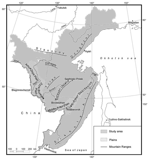
Figure 1.
The topography of the southern part of the Russian Far East.
As the study region stretches along the coast of the Pacific Ocean from south to north, it has from Warm Summer Continental to Subarctic Continental Climates, according to the Köppen-Geiger climatic classification [83,84]. An extreme continental annual temperature regime typifies the climate of the area. The annual temperature norm (1961–1990) varies between –5.4 °C at Ekimchan to 5.7 °C at Pogranichnyi, and the annual temperature ranges change from 28.2 °C over the coastal zone to 52.7 °C in the continental interior [44].
The aily maximum and minimum air temperatures from a network of 50 weather stations (Table 1) across the study region were used to generate GDD and GDDSI for the period 1966 to 2017. The minimum and maximum temperatures for each day are those recorded by minimum and maximum thermometers.

Table 1.
Weather stations in the Russian Far East region used in the current study.
3.2. Method
GDD is an index linked to plant development, reflecting the fact that growth will take place only when the temperature is above a certain threshold for a specified number of days. The construction of GDD incorporates information on both the passage of time and the temperature experienced by a plant during the growing season. It is a widely used temperature-related agro-climatic indicator since a change in GDDs can lead to significant changes in the phenology of plants and, consequently, changes in agricultural production. It is a measure of the heat a plant needs to produce a successful crop. A limitation is that it does not take in account other environmental factors and different responses of plants to the same temperature during various stages of their growth; nevertheless, it has been shown to be useful in agricultural, phenological and other applications [42,44,46,59]. For instance, GDDs have been used to predict the growth stages of a variety of crops, mid-latitude crops in particular, such as maize, wheat and soya bean; it is also useful in planning defensive actions against insects and diseases that negatively affect crops [40,41,42,46,48,85,86].
There are several ways of calculating GDD; each model has its strengths and weaknesses [86]. To achieve the goal of the current research, we used the approach suggested by Grigorieva et al. [44], where the number of growing degree days required for plant growth and maturation (GDD) is given by
where Ti is the mean air temperature (°C), Tmax is the daily maximum air temperature (°C), Tmin is the daily minimum air temperature (°C), Tbase is the base or threshold temperature (°C), and i = 1, 2, … m—days with a higher threshold temperature Tbase during the growing season.
Ti = (Tmax + Tmin)/2
Plants adapt to climatic conditions over time; they develop best above a certain temperature below which there is little or no plant growth. However, each crop type has its own base temperature threshold (Tbase) [44]. Because of the close connection of 0, 5, 10 and 15 °C limits with the onset and end of the crop growth, these temperatures are normally used as the threshold or base temperatures in common estimations of thermal influence on plants [41,44,50]. Based on Gordeev et al. [50], the following descriptions are applied:
- >0 °C:
- onset of ‘warm season’;
- >5 °C:
- commencement of period of active crop growth;
- >10 °C:
- beginning of period for the cold-resistant crop development;
- >15 °C:
- conditions suited to heat-reliant plants.
A comparison with Tbase must be done individually for Tmax and Tmin before calculating the mean value: if Tmax < Tbase then Tmax = Tbase, and if Tmin < Tbase then Tmin = Tbase.
The matter of upper threshold temperature is important as it is well known that the hot-season upper limit of 35 °C has significance for various agricultural impacts, such as heat shock in wheat [87]. High air temperatures may considerably decrease plant growth and development rates or even suppress growth [46,48,86]. There are various ways of estimation this, discussed in detail in Grigorieva et al. [44]. In the current work, the method using a horizontal high-temperature threshold cut-off with upper threshold of 30 °C (TUT) is applied as explained by Matzarakis et al. [85]. All values Ti, Tmax or Tmin are thrown off to TUT if they surpass TUT [44,85].
The concept of a GDD Sensitivity Index (GDDSI) is used to assess the sensitivity of agricultural practices to changed thermal conditions. GDDSI is defined as the percentage change in GDD for a particular warming scenario. In light of the above discussion of crop sensitivity and thermal thresholds, GDDSI is calculated for GDD to base 0 °C (GDD0), 5 °C (GDD5), 10 °C (GDD10), and 15 °C (GDD15).
Three warming scenarios +1, +2 and +3 °C are used with thresholds similar to those used elsewhere by adding 1, 2 or 3 °C to daily temperatures at each site [66]. According to Hennessy and Pittock [66], this presupposes that daily temperature variation and autocorrelation remain the same; although, in reality, things will be more complex. GDDSI is expressed as a percentage of the base value. For example, taking GDD15, GDDSI for the +3 °C scenario is
where GDD15 is calculated using data for the period 1966–2017. CCSI maps for various GDDSI scenarios are produced to provide a concise summary of the impact on the spatial redistribution of crop growth due to changed climatic conditions.
GDD15SI+3 = GDD15+3/GDD15 × 100
4. Results
To begin with, four threshold temperatures were applied for GDD calculations with results shown in Supplementary Materials, Table S1, along with standard deviations for each GDD, and in maps (Figure 2). The base temperature 0 °C (GDD0) indicates the beginning of the warm or growing season. The coastal locations along the cold sea shore of the Sea of Japan and the Okhotsk Sea show the maritime influence of the Pacific Ocean with sufficiently lower values and are more than two times lower than in continental locations in the southern portion of the study area; GDD0 in elevated locations has intermediate values (Figure 2A).
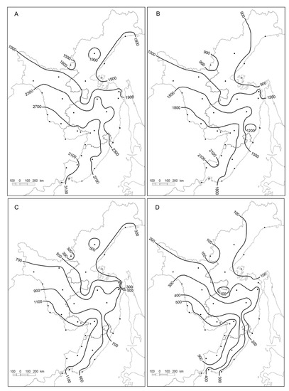
Figure 2.
Growing degree days (GDD) in the Russian Far East for period 1966–2017 for four thresholds: (A) GDD0, (B) GDD5, (C) GDD10, and (D) GDD15.
The 5 °C temperature threshold (GDD5) marks the beginning of the period with active growth of a plant. Spatial distribution of GDD5 is similar to GDD0 (Figure 2B). The values of GDD5 range from nearly 700 °C in Okhotsk in the northern coastal part of the study area to GDD5 more than 2100 over the continental locations at the south with almost thrice the spatial differences. The coldest areas are in the elevated regions of the north-west and in the mountains.
The spatial variability of GDD10 characterizes the onset of the main period of active growth for most crops. The highest values found in the far south, which are almost five times higher than at the north (Figure 2C). There is a big difference in GDD10 between continental and coastal parts at roughly the same latitude. Southern locations show a 2.3 times difference, with Yekaterino-Nickolskoe (1226 °C) versus to Zolotoy (520 °C) as an example. The contrast in the far north is not as large when GDD10 in inland elevated areas are compared with the coastal regions (Figure 2C).
The best climatic conditions for heat-reliant plants are described by GDD15. The difference in GDD15 between the north and the south of the region is up to 11 times, from about 20 °C in Okhotsk to more than 600 °C in Sviyagino. This illustrates the great contrast in the conditions between the two geographical extremes in the summer (Figure 2D). The spatial pattern is similar to that described for GDD0, GDD5 and GDD10, but with considerably lower absolute values, where isotherm boundaries reflect topographical and coastal influences (Figure 1).
There is a positive relationship between the value of growing degree days for 5, 10 and 15 °C thresholds and its standard deviation (SD), and this association is more pronounced for the higher threshold of 15 °C (Figure 3).
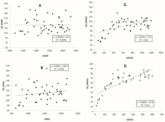
Figure 3.
Relationship between growing degree days (GDD) for locations in the Russian Far East for period 1966–2017 for four thresholds: (A) GDD0, (B) GDD5, (C) GDD10, and (D) GDD15, and correspondent standard deviation (SD).
Both GDDs and standard deviations depend on the latitude of the location, and this dependence is apparent for all temperature thresholds. As an example, we show the plots for GDD15 and corresponding values of SD. Figure 4 demonstrates the relationship between GDD15 and its SD with latitude: the further to the north, the lower the GDD15, with SD showing results for the continental weather stations (Figure 4A,B) and for maritime locations (Figure 4C,D). The response of both GDD15 and its SD on latitude is more evident for the coastal weather stations.
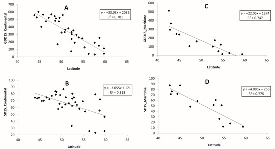
Figure 4.
Relationship between growing degree days with 15 °C threshold (GDD15), its standard deviation (SD15) and latitude for locations in the Russian Far East for period 1966–2017: (A,B) continental weather stations, (C,D) maritime weather stations.
Outputs for GDDSI are given in Supplementary Materials, Table S2, keeping in mind that GDDSI is defined as the percentage change in GDD using Equation (3) for three warming scenarios (+1, +2, +3 °C) and four GDD base thresholds (GDD0, GDD5, GDD10 and GDD15). The results show the non-linear response of GDDs to incremental warming depending on base temperatures. GDDSI for the threshold of 0 °C gives values from 7% to 13% for +1 °C; from 5% to 27% for +2 °C; and from 20% to 41% for the +3 °C scenario. Sensitivity for the 5 °C base temperature delivers slightly higher values: from 9–20% to 6–41% and 25–65% for the +1, +2, +3 °C warming scenarios, respectively. Considerably bigger results can be found for GDD10 with 12–40%, 5–88% and 33–142%. The highest sensitivity is shown for the GDD15: 19–153%, 4–496%, and as high as 65%—more than 1000% for the +3 °C warming scenario. The results indicate that the higher the base threshold, the higher the sensitivity. Highest sensitivity is for GDD15 at Okhotsk in the far north.
In general, sensitivity does not increase significantly as warming rate increases. In Skovorodino, Yekaterino-Nickolskoye and Sviyagino (all inland locations) sensitivity varies from 7 to 65–66, versus Bolshoy Shantar and Okhotsk, maritime areas, where sensitivity fluctuates from 12–13 to 800–1000.
It is interesting to note the lower sensitivity for the +2 °C warming scenario compared with +1 °C at some southern continental weather stations. Examples of this are Timiryazevskyi and Dalnerechensk, which can be explained by the cut off when daily temperatures exceed the upper threshold of 30 °C in very hot summer conditions. Except for those cases, generally larger values are found for the higher thresholds and the higher warming scenario.
Both sensitivity indices and their standard deviations depend on the latitude of the location, its elevation and proximity to the coastline. Figure 5, Figure 6, Figure 7 and Figure 8 show the results of +3 °C warming for two thresholds, 0 °C (Figure 5 and Figure 6) and 15 °C (Figure 7 and Figure 8).
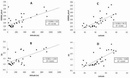
Figure 5.
Dependence of Sensitivity Index for growing degree days with 0 °C threshold (GDD0SI) and its standard deviation (SD) for a GDD0+3 scenario on altitude and latitude for continental locations in the Russian Far East for the period 1966–2017: (A,B) altitude (m), (C,D) latitude.
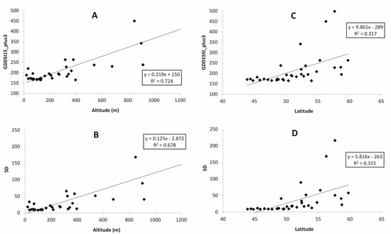
Figure 6.
Dependence of Sensitivity Index for growing degree days with 15 °C threshold (GDD15SI) and its standard deviation (SD) for a GDD15+3 scenario on altitude and latitude for continental locations in the Russian Far East for the period 1966–2017: (A,B) altitude (m), (C,D) latitude.
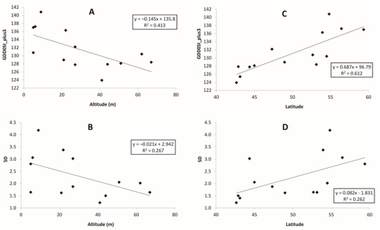
Figure 7.
Dependence of Sensitivity Index for growing degree days with 0 °C threshold (GDD0SI) and its standard deviation (SD) for a GDD0+3 scenario on altitude and latitude for maritime locations in the Russian Far East for the period 1966–2017: (A,B) altitude (m), (C,D) latitude.
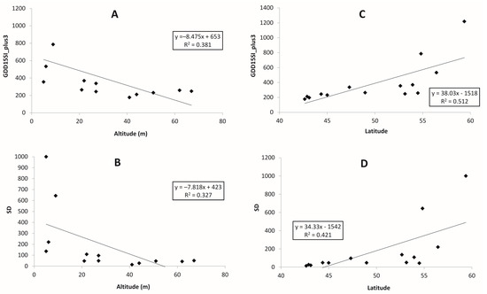
Figure 8.
Dependence of Sensitivity Index for growing degree days with 15 °C threshold (GDD15SI) and its standard deviation (SD) for a GDD15+3 scenario on altitude and latitude for maritime locations in the Russian Far East for the period 1966–2017: (A,B) altitude (m), (C,D) latitude.
The relationship for 5 and 10 °C is very similar. Sensitivity indices for continental stations depend on their altitude: the higher the location, the greater the sensitivity, and this relationship shows up for all temperature thresholds for both sensitivity indices and their temporal variability, whereas the effect on latitude is less pronounced (Figure 5 and Figure 7). The climate sensitivity at maritime locations for all temperature thresholds depends on latitude: the further north, the higher sensitivity (Figure 6 and Figure 8).
Mapped Results
One of the aims of the study was to produce CCSI maps that set apart zones of different magnitudes of sensitivity to climate change. The results show areas of high and low sensitivity to change as well as the relative level of the potential effect. To describe the spatial distribution of temperature sensitivity to warming, Figure 9 and Figure 10 give the maps of CCSI: a GDD5+3 scenario in Figure 9, illustrating GDD5SI+3 for the study area, where GDD5SI+3 = GDD5+3/GDD5 × 100.
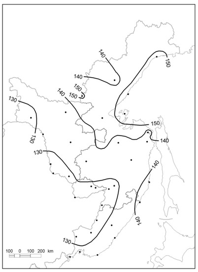
Figure 9.
CCSI map for a GDD5+3 scenario showing GDD5SI+3 for the Russian Far East, where GDD5SI+3 = GDD5+3/GDD5 × 100. The areas bounded by isolines indicate zones of increasing sensitivity expressed as the percentage change in GDDs5 brought about by the changed climatic conditions.
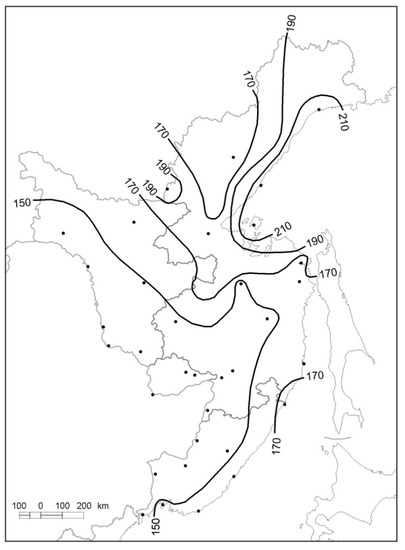
Figure 10.
CCSI map for a GDD10+3 scenario showing GDD10SI+3 for the Russian Far East study area, where GDD10SI+3 = GDD10+3/GDD10 × 100. The areas bounded by isolines indicate zones of increasing sensitivity expressed as the percentage change in GDDs10 brought about by the changed climatic conditions.
The areas bounded by isolines indicate zones of increasing sensitivity expressed as the percentage change in GDDs brought about by the changed climatic conditions. Figure 10 shows spatial pattern for a GDD10+3 scenario with much higher values but with very similar spatial variations.
Sensitivity to a warming shows the inverse relationship to the temperature: the higher the value of the GDD, the lower the sensitivity index. Figure 11 shows the results for the GDD15 for all warming scenarios with the relationship more pronounced for the higher +3 °C warming scenario. In all cases, the colder the climate, the higher the sensitivity to the warming, as would be expected, although the extent of the effect varies.
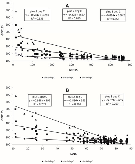
Figure 11.
Relationship between growing degree days with 15 °C threshold (GDD15), its standard deviation (SD15) and Sensitivity Index (GDD15SI) for locations in the Russian Far East for the period 1966–2017 for +1, +2 and +3 °C warming scenarios: (A) for GDD15, (B) for SD15.
Changes in sensitivity are also influenced by the standard deviation. Figure 11B demonstrates the same dependence of the sensitivity index on the temporal variability of GDD: the larger the standard deviation, the lower the sensitivity index. A general rule is that for sites with currently similar GDD, the impact of each degree of warming is greater when the mean and the standard deviation are smaller.
Figure 12 shows the dependence of sensitivity of GDDS with regard to temporal and spatial variability. Using GDD15 is an example typical of all warming scenarios; Figure 12A is plotted for the SD near 25, which shows the weakest relationship with sensitivity. The strength of the relationship increases with rising of the SD: Figure 12B shows the results for an SD near 55, while Figure 12C,D—for SD near 75 and 85, respectively. At places with the same standard deviation, the sites with lower values of GDDs are more sensitive and this relationship is more apparent for the larger warming scenario.
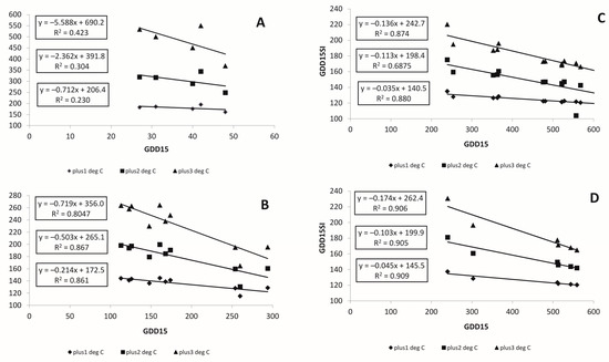
Figure 12.
Relationship between growing degree days with 15 °C threshold (GDD15) and Sensitivity Index (GDD15SI) depending on its standard deviation (SD15) for locations in the Russian Far East for the period 1966–2017 for +1, +2 and +3 °C warming scenarios: (A) for SD15 near 25, (B) for SD15 near 55, (C) for SD15 near 75, (D) for SD15 near 85.
5. Discussion
The thermal supply of the region expressed in GDD values varies spatially and as a whole, follows the main geographical patterns of temperature distribution moderated proximity to large water bodies (Amur River and the Pacific Ocean), coastline and relative relief of the land. Generally, the magnitude of the GDD increases from north to south and decreases towards the coast. It also decreases from lowland areas to higher land. The gradient is less further to the north due to the influence of elevated terrain and its spatial distribution. The most noticeable spatial gradient is for locations at similar latitudes, which is explained by the distance from the coastal waters of the Pacific Ocean.
Since the study area is covered by discontinuous permafrost at the north and is characterized by long-term seasonal soil freezing, or sporadic permafrost in mountains at the middle [88], only plains at the southern part can be used for crop production [50]. Our study confirms previous research that heat supply here is sufficient for grain crops (wheat, oats, barley, and even rice at the southernmost locations), vegetables and soybeans [23,44,50,57]. As it is very cold in winter and snow cover is low, only spring varieties are grown. Due to low thermal resources at places in the north, in the mountains and at the coastal locations, they are good enough only for some forage crops and potatoes and for cultivating vegetables in greenhouses [44].
CCSI maps show zones of different degrees of sensitivity to global warming by revealing the changed spatial redistribution of climate-determined temperature resources for agriculture. The method allows the estimation of temperature resource change for zones within the study area. The results show the size and location of impact. On the whole, the larger the GDDSI, the more sensitive the climate is to warming in terms of crop growing conditions. In most cases, sensitivity does not increase significantly as the warming rate increases.
Different places respond to warming in different ways. Both CCSI maps (Figure 9 and Figure 10) show the dependence of sensitivity indices on the closeness to the coast line and relief of the area, reflecting the effects of both mountain ranges and plains (Sikhote-Alin and Dzugdzur, Middle-Amur Plain and Low-Amur Depression, Figure 1). A noticeable feature of the study is that the sensitivity generally increases from south to north: the colder the climate the higher the sensitivity to the warming; it varies considerably from one location to another—especially coastal versus continental locations.
For sites that have a similar GDD, the effect of each degree of warming is greater where both the mean and the standard deviation are lower. These results are in contrast to those of Hennessy and Pittock [66], who found that the response to incremental warming is greater where the mean temperature is higher and the standard deviation is lower, and where the warmer sites are more sensitive for sites with the same standard deviation. At sites with the same standard deviation, those with lower GDDs are more sensitive and this relationship is more conspicuous for higher warming scenarios.
The method used represents the sensitivity of crop yield using percentage changes in GDD with average temperatures change, which is quite effective only in regions where plant growth is strongly constrained by thermal supply, without moisture restrictions. This definition of sensitivity makes sense only where plant growth is strongly and nearly linearly related to accumulated temperature. It would probably not be applied in agricultural regions where heat is always sufficient, with excess heat and moisture supply being the main limiting factors.
The region studied presents a strong heat limited regime. The results confirm that GDD is a robust agro-climatic indictor of the impact temperature change at the regional scale on crop growth in a thermally extreme mid-latitude climate. This coincides with the findings [39,43,45,61,63,64] in different climates regimes. Clearly, a full impact assessment should include the role of other climate variables such as precipitation and soil moisture deficit, evapotranspiration, solar radiation [39,45,64]. However, research on annual and especially warm-period precipitation trends for the Russian Far East, characterized by very high precipitation in summer time show insignificant impact compared to inter-annual variability of climate [89]. This suggests a minor role of changes in precipitation versus a major impact temperature on the functioning of plant ecosystems in the study area, the reason our research is focused on changes of thermal supply only.
In our approach, we assume variability will remain unchanged. However, climate variability changed through past decades, so we might expect the same in a warming future. In fact, future climate is expected to manifest itself in temperature regimes that are more complex, involving changes in the temperature distribution, changes in the seasonality of the temperature, and changes in temperature extremes. Nevertheless, the methodology presented in this study is attractive as it is uncomplicated. Furthermore, temperature thresholds and warming scenarios can be adjusted as required. In areas of highly variable topography, or those in close proximity to large water bodies, the sensitivity to warming can be deduced from shifts in risk boundaries.
Although the topography of the study region is very complex, some general spatial patterns can be defined. For instance, since agricultural thermal supply is generally declining northward, the same absolute temperature increase has a greater relative impact on crop potential at higher latitudes than at lower latitudes. Regions with higher sensitivity to heat supply at higher thermal thresholds are likely to have more advantages due to the warming effect, which can be used in adaptation strategies, e.g., when predicting farm investments in crop production in northern or coastal areas. In case of future climate changes, local governments should take appropriate agricultural management measures to reduce its negative impact on crop production. If we forecast an increase in heat supply, the adaptation program should include appropriate spatial redistribution of crops, shifting agricultural production further north, introducing crop varieties adapted to warmer conditions, etc. [8,11,23,36]. In some cases, warmer and milder summers might have a beneficial effect on plant development, creating favorable conditions for certain crops [11,23]. The method used in study enables the evaluation of impact potential without having to continually re-run transfer functions. Non-climate experts such as planners and other decision makers can use the schemes to assess and re-assess impact according to their expectation of climate change or variability and review the relative merits of various response and/or adjustment strategies [13,38]. As there are no comparable studies in the literature on similar climatic regions and at equivalent latitudes, further research may produce results on which comparisons can be valuably made.
6. Conclusions
The present study examines the utility of GDDs and its changes as an agro-climatic indicator of the sensitivity to climate change at the regional scale in a thermally extreme mid-latitude climate, namely, the vast area that is the Russian Far East, the region with the largest annual temperature amplitude.
GDDSI, defined as the percentage change in GDD for a particular warming scenario, is used to assess the sensitivity of agricultural practices to changed thermal conditions. Generally, sensitivity increases from south to north: the colder the climate the higher the sensitivity to the warming; the highest sensitivity is for GDDs with a threshold at 15 °C in the far north of the study area where conditions currently are marginal for crop growth. More specifically, GDDSI can serve as a measure of the likely success in the growth of a particular crop.
CCSI maps for various warming scenarios are produced to provide a concise summary of the impact, indicating magnitude of the potential impact due to changed climatic conditions, and its possible effect on the spatial redistribution of crop growth. The results provide a basis for identifying sensitive regions in climate change vulnerability assessments.
The methodology used in sensitivity studies such as presented here is both straightforward and flexible. Any of a variety of threshold temperatures can be used depending on the purpose of the research and nature of the impact assessment. Moreover, sensitivity to a changed climate in places with highly variable topography can be construed from shifts in boundaries of isotherms and impact risks considered. Clearly, however, a comprehensive impact assessment would have to incorporate other climatic variables, such as precipitation and evapotranspiration, along with temperature. Further research should be done to estimate the impact of possible adaptation measures in the long-run perspective, and their efficiency on the Russian agriculture as a whole.
Supplementary Materials
The following are available online at https://www.mdpi.com/2073-4433/11/4/404/s1, Table S1: Growing degree days (GDD) for locations in Russian Far East for period 1966–2017 for four thresholds, namely, GDD0, GDD5, GDD10, and GDD15, and standard deviation SD, Table S2: GDDSI for three warming scenarios (+1, +2, +3 °C) and four GDD base thresholds (GDD0, GDD5, GDD10 and GDD15).
Funding
This research received no external funding and was performed according to the topic research of ICARP FEB RAS.
Acknowledgments
This research is dedicated to the memory of Chris de Freitas (1948–2017), who provided extremely valuable insights and ideas about the testing and application of the GDDSI.
Conflicts of Interest
The author declares no conflict of interest.
References
- Smith, J.B.; Schellnhuber, H.-J.; Mirza, M.M.Q. Vulnerability to climate change and reasons for concern: A synthesis. In Climate Change 2001: Impacts, Adaptation and Vulnerability. IPCC Working Group II; McCarthy, J.J., Canziani, O., Leary, N.A., Dokken, D.J., White, K.S., Eds.; Cambridge University Press: Cambridge, UK, 2001; pp. 914–967. [Google Scholar]
- Robinson, J.; Bradley, M.; Busby, P.; Connor, D.; Murray, A.; Sampson, B.; Soper, W. Climate change and sustainable development: Realizing the opportunity. AMBIO J. Human Environ. 2006, 35, 2–9. [Google Scholar] [CrossRef]
- United Nations. Transforming our World: The 2030 Agenda for Sustainable Development. 2015. Available online: https://sustainabledevelopment.un.org/content/documents/21252030%20Agenda%20for%20Sustainable%20Development%20web.pdf (accessed on 10 March 2020).
- Boswell, M.R.; Greve, A.I.; Seale, T.L. Climate Change Vulnerability Assessment. In Climate Action Planning; Island Press: Washington, DC, USA, 2019. [Google Scholar] [CrossRef]
- IPCC. 2014: Climate Change 2014: Synthesis Report. Contribution of Working Groups I, II and III to the Fifth Assessment Report of the Intergovernmental Panel on Climate Change; Core Writing Team, Pachauri, R.K., Meyer, L.A., Eds.; IPCC: Geneva, Switzerland, 2014; p. 151. Available online: https://epic.awi.de/id/eprint/37530/1/IPCC_AR5_SYR_Final.pdf (accessed on 10 March 2020).
- Adger, W.N. Vulnerability. Glob. Environ. Chang. 2006, 16, 268–281. [Google Scholar] [CrossRef]
- Füssel, H.-M. Review and Quantitative Analysis of Indices of Climate Change Exposure, Adaptive Capacity, Sensitivity, and Impacts; World Bank: Washington, DC, USA, 2010; Available online: https://openknowledge.worldbank.org/bitstream/handle/10986/9193/WDR2010_0004.pdf?sequence=1&isAllowed=y (accessed on 10 March 2020).
- Parry, M.; Carter, T. The Assessment of Effects of Climatic Variations on Agriculture: Aims, Methods and Summary of Results. In The Impact of Climatic Variations on Agriculture; Vol. 1: Assessment in cool temperate and cold regions; Parry, M.L., Carter, T.R., Konijn, N.T., Eds.; Springer: Dordrecht, The Netherlands, 1988; pp. 11–96. [Google Scholar] [CrossRef]
- Anwar, M.R.; Feng, H.; Macadam, I.; Kelly, G. Adapting agriculture to climate change: A review. Theor. Appl. Clim. 2013, 113, 225–245. [Google Scholar] [CrossRef]
- Parry, M.L.; Carter, T.R.; Konijn, N.T. Planned Responses in Agricultural Management under a Changing Climate. In The Impact of Climatic Variations on Agriculture; Parry, M.L., Carter, T.R., Konijn, N.T., Eds.; Springer: Dordrecht, The Netherlands, 1988. [Google Scholar] [CrossRef]
- Parry, M.N. Climate Change and World Agriculture; Earthscan: London, UK, 1990. [Google Scholar] [CrossRef]
- de Freitas, C.R.; Helbig, M.; Matzarakis, A. Hydroclimatic assessment of water resources of low Pacific islands: Evaluating sensitivity to climatic change and variability. Int. J. Clim. 2014, 34, 881–892. [Google Scholar] [CrossRef]
- Bannayan, M.; Paymard, P.; Ashraf, B. Vulnerability of maize production under future climate change: Possible adaptation strategies. J. Sci. Food Agric. 2016, 96, 4465–4474. [Google Scholar] [CrossRef]
- Wall, E.; Smit, B. Climate Change Adaptation in Light of Sustainable Agriculture. J. Sustain. Agric. 2005, 27, 113–123. [Google Scholar] [CrossRef]
- Springmann, M.; Charles, H.; Godfray, J.; Rayner, M.; Scarborough, P. Analysis and valuation of the health and climate change cobenefits of dietary change. Proc. Natl. Acad. Sci. USA 2016, 113, 4146–4151. [Google Scholar] [CrossRef]
- Farooq, M.; Rehman, A.; Pisante, M. Sustainable Agriculture and Food Security. In Innovations in Sustainable Agriculture; Farooq, M., Pisante, M., Eds.; Springer: Cham, Switzerland, 2019. [Google Scholar] [CrossRef]
- Paloviita, A.; Järvelä, M. Multilevel Governance for Climate Change Adaptation in Food Supply Chains. In Sustainable Solutions for Food Security; Sarkar, A., Sensarma, S., vanLoon, G., Eds.; Springer: Cham, Switzerland, 2019. [Google Scholar] [CrossRef]
- Praveen, B.; Sharma, P. A review of literature on climate change and its impacts on agriculture productivity. J. Public Aff. 2019, e1960. [Google Scholar] [CrossRef]
- Tian, Z.; Xu, H.; Zhong, H.; Sun, L.; Liu, J. Agricultural Adaptation to Climate Change in China. In Adaptation to Climate Change in Agriculture; Iizumi, T., Hirata, R., Matsuda, R., Eds.; Springer: Singapore, 2019. [Google Scholar] [CrossRef]
- Pandey, D. Agricultural Sustainability and Climate Change Nexus. In Contemporary Environmental Issues and Challenges in Era of Climate Change; Singh, P., Singh, R., Srivastava, V., Eds.; Springer: Singapore, 2020. [Google Scholar] [CrossRef]
- Barnett, J. Adapting to Climate Change in Pacific Island Countries: The Problem of Uncertainty. World Dev. 2001, 29, 977–993. [Google Scholar] [CrossRef]
- Smit, B.; Pilifosova, O. Adaptation to climate change in the context of sustainable development and equity. In Climate Change 2001: Impacts, Adaptation and Vulnerability. IPCC Working Group II; McCarthy, J.J., Canziani, O., Leary, N.A., Dokken, D.J., White, K.S., Eds.; Cambridge University Press: Cambridge, UK, 2001; pp. 877–912. [Google Scholar]
- Belyaeva, M.; Bokusheva, R. Will climate change benefit or hurt Russian grain production? A statistical evidence from a panel approach. Clim. Chang. 2018, 149, 205. [Google Scholar] [CrossRef]
- de Freitas, C.R.; Fowler, A.M. Identifying sensitivity to climatic change at the regional scale: The New Zealand example. In Proceedings of the 15th Conference New Zealand Geographical Society; New Zealand Geographical Society Conference Series No 15; Welch, R., Ed.; New Zealand Geographical Society: Dunedin, New Zealand, 1989; pp. 254–261. [Google Scholar]
- Zhou, Y.; Li, N.; Dong, G.; Wu, W. Impact assessment of recent climate change on rice yields in the Heilongjiang Reclamation Area of north-east China. J. Sci. Food Agric. 2013, 93, 2698–2706. [Google Scholar] [CrossRef]
- Anderton, S.; Latron, J.; Gallart, F. Sensitivity analysis and multi-response, multi-criteria evaluation of a physically based distributed model. Hydrol. Process. 2002, 16, 333–353. [Google Scholar] [CrossRef]
- van Vliet, M.T.H.; Ludwig, F.; Zwolsman, J.J.G.; Weedon, G.P.; Kabat, P. Global river temperatures and sensitivity to atmospheric warming and changes in river flow. Water Resour. Res. 2011, 47, W02544. [Google Scholar] [CrossRef]
- Sreedevi, S.; Eldho, T.I. A two-stage sensitivity analysis for parameter identification and calibration of a physically-based distributed model in a river basin. Hydrol. Sci. J. 2019. [Google Scholar] [CrossRef]
- McCuen, R.H. A sensitivity and error analysis of procedures used for estimating evaporation. JAWRA J. Am. Water Resour. Assoc. 1974, 10, 486–498. [Google Scholar] [CrossRef]
- Saxton, K.E. Sensitivity analysis of the combination evapotranspiration equation. Agric. Meteorol. 1975, 15, 343–353. [Google Scholar] [CrossRef]
- Gong, L.; Xu, C.-Y.; Chen, D.; Halldin, S.; Chen, Y.D. Sensitivity of the Penman–Monteith reference evapotranspiration to key climatic variables in the Changjiang (Yangtze River) basin. J. Hydrol. 2006, 329, 620–629. [Google Scholar] [CrossRef]
- Gao, Z.; He, J.; Dong, K.; Bian, X.; Li, X. Sensitivity study of reference crop evapotranspiration during growing season in the west Liao River basin, China. Theor. Appl. Clim. 2016, 124, 865–881. [Google Scholar] [CrossRef]
- Nouri, M.; Homaee, M.; Bannayan, M. Quantitative Trend, Sensitivity and Contribution Analyses of Reference Evapotranspiration in some Arid Environments under Climate Change. Water Resour. Manag. 2017, 31, 2207–2224. [Google Scholar] [CrossRef]
- Paparrizos, S.; Maris, F.; Matzarakis, A. Sensitivity analysis and comparison of various potential evapotranspiration formulae for selected Greek areas with different climate conditions. Theor. Appl. Clim. 2017, 128, 745–759. [Google Scholar] [CrossRef]
- Ebi, K.L.; Hasegawa, T.; Hayes, K.; Monaghan, A.; Paz, S.; Berry, P. Health risks of warming of 1.5 °C, 2 °C, and higher, above pre-industrial temperatures. Environ. Res. Lett. 2018, 13, 063007. [Google Scholar] [CrossRef]
- Sirotenko, O.D.; Abashina, H.V.; Pavlova, V.N. Sensitivity of the Russian agriculture to changes in climate, CO2 and tropospheric ozone concentrations and soil fertility. Clim. Chang. 1997, 36, 217. [Google Scholar] [CrossRef]
- Kryza, M.; Szymanowski, M.; Błaś, M.; Migała, K.; Werner, M.; Sobik, M. Observed changes in SAT and GDD and the climatological suitability of the Poland-Germany-Czech Republic transboundary region for wine grapes cultivation. Theor. Appl. Clim. 2015, 122, 207–218. [Google Scholar] [CrossRef]
- Lin, Y.; Wu, W.; Ge, Q. CERES-Maize model based simulation of climate change impacts on maize yields and potential adaptive measures in Heilongjiang Province, China. J. Sci. Food Agric. 2015, 95, 2838–2849. [Google Scholar] [CrossRef]
- Graczyk, D.; Kundzewicz, Z.W. Changes of temperature-related agroclimatic indices in Poland. Theor. Appl. Clim. 2016, 124, 401–410. [Google Scholar] [CrossRef]
- Russelle, M.P.; Wilhelm, W.W.; Olson, R.A.; Power, J.F. Growth analysis based on degree days. Crop. Sci. 1984, 24, 28–32. [Google Scholar] [CrossRef]
- Gordon, R.; Bootsma, A. Analyses of growing degree-days for agriculture in Atlantic Canada. Clim. Res. 1993, 3, 169–176. [Google Scholar] [CrossRef]
- Førland, E.J.; Skaugen, T.E.; Benestad, R.E.; Hanssen-Bauer, I.; Tveito, O.E. Variations in thermal growing, heating, and freezing indices in the Nordic Arctic, 1900–2050. Arct. Antarct. Alp. Res. 2004, 36, 347–356. [Google Scholar] [CrossRef]
- Gavilán, R.G. The use of climatic parameters and indices in vegetation distribution. A case study in the Spanish Sistema Central. Int. J. Biometeorol. 2005, 50, 111–120. [Google Scholar] [CrossRef]
- Grigorieva, E.A.; Matzarakis, A.; de Freitas, C.R. Analysis of the growing degree days as a climate impact indicator in a region with extreme annual air temperature amplitude. Clim. Res. 2010, 42, 143–154. [Google Scholar] [CrossRef]
- Wang, L.; Deng, H.; Qiu, X.; Wang, P.; Yang, F. Determining the impact of key climatic factors on geographic distribution of wild Akebia trifoliate. Ecol. Indic. 2020, 112, 106093. [Google Scholar] [CrossRef]
- Wang, J.Y. A critique of the heat-unit approach to plant response studies. Ecology 1960, 41, 785–790. [Google Scholar] [CrossRef]
- Schwartz, M.D.; Ahas, R.; Aasa, A. Onset of spring starting earlier across the Northern Hemisphere. Glob. Chang. Boil. 2006, 12, 343–351. [Google Scholar] [CrossRef]
- Bootsma, A. Long term (100 year) climatic trends for agriculture at selected locations in Canada. Clim. Chang. 1994, 26, 65–88. [Google Scholar] [CrossRef]
- Bootsma, A.; Anderson, D.; Gameda, S. Potential impacts of climate change on agroclimatic indices in southern regions of Ontario and Quebec. In Technical Bulletin ECORC Contribution; Eastern Cereal and Oilseed Research Centre: Ottawa, ON, Canada, 2004; No.03–284. [Google Scholar]
- Gordeev, A.V.; Kleschenko, A.D.; Chernyakov, B.A.; Sirotenko, O.D. Bioclimatical Potential of Russia: Theory and Practice; Association of Scientific Publications KMK: Moscow, Russia, 2006; p. 512. (In Russian) [Google Scholar]
- Hall, A.; Jones, G.V. Effect of potential atmospheric warming on temperature-based indices describing Australian winegrape growing conditions. Aust. J. Grape Wine Res. 2009, 15, 97–119. [Google Scholar] [CrossRef]
- Cabré, F.; Nuñez, M. Impacts of climate change on viticulture in Argentina. Reg. Environ. Chang. 2020, 20, 12. [Google Scholar] [CrossRef]
- Tonietto, J.; Carbonneau, A. A multicriteria climatic classification system for grape-growing regions worldwide. Agric. For. Meteorol. 2004, 124, 81–97. [Google Scholar] [CrossRef]
- Yoshino, M.M.; Horie, T.; Seino, H.; Tsujii, H.; Uchijima, T.; Uchijima, Z. The Effects of Climatic Variations on Agriculture in Japan. In The Impact of Climatic Variations on Agriculture; Vol. 1. Assessment in Cool Temperate and Cold Regions; Parry, M.L., Carter, T.R., Konijn, N.T., Eds.; Kluwer Acad. Publ.: Dordrecht, The Netherlands, 1988; pp. 723–868. [Google Scholar]
- Holdridge, L.R. Life Zone Ecology; Tropical Science Center: San Jose, Costa Rica, 1967. [Google Scholar]
- Wang, J. Modelling the Distribution of Five Caragana Species in Temperate Northern China. Chin. J. Plant Ecol. 2009, 33, 12–24. [Google Scholar]
- Pitovranov, S.E.; Iakimets, V.; Kiselev, V.I.; Sirotenko, O.D. The effects of climatic variations on agriculture in the subarctic zone of the USSR. In The Impact of Climatic Variations on Agriculture; Vol. 1, Assessments in cool temperate and cold regions; Parry, M.L., Carter, T.R., Konijn, N.T., Eds.; Kluwer: Dordrecht, The Netherlands, 1988; pp. 617–722. [Google Scholar]
- Malheiro, A.C.; Santos, A.S.; Helder, F.; Pinto, J.G. Climate change scenarios applied to viticultural zoning in Europe. Clim. Res. 2010, 43, 163–177. [Google Scholar] [CrossRef]
- Karl, T.R.; Jones, P.D.; Knight, R.W.; Kukla, G.; Plummer, N.; Razuvayev, V.; Gallo, K.P.; Lindesay, J.; Charlson, R.J.; Peterson, T.C. Asymmetric trends of daily maximum and minimum temperature. Bull. Am. Meteorol. Soc. 1993, 74, 1007–1023. [Google Scholar] [CrossRef]
- Jones, P.D.; Briffa, K.R. Growing season temperatures over the former Soviet Union. Int. J. Clim. 1995, 15, 943–959. [Google Scholar] [CrossRef]
- Su, L.; Wang, Q.; Bai, Y. An analysis of yearly trends in growing degree days and the relationship between growing degree day values and reference evapotranspiration in Turpan area, China. Theor. Appl. Clim. 2013, 113, 711–742. [Google Scholar] [CrossRef]
- Spinoni, J.; Vogt, J.; Barbosa, P. European degree-day climatologies and trends for the period 1951–2011. Int. J. Clim. 2015, 35, 25–36. [Google Scholar] [CrossRef]
- Zhao, D.; Wu, S. Spatial and temporal variability of key bio-temperature indicators on the Qinghai-Tibetan Plateau for the period 1961–2013. Int. J. Clim. 2016, 36, 2083–2092. [Google Scholar] [CrossRef]
- Paparrizos, S.; Matzarakis, A. Present and future responses of growing degree days for Crete Island in Greece. Adv. Sci. Res. 2017, 14, 1–5. [Google Scholar] [CrossRef]
- Wypych, A.; Sulikowska, A.; Ustrnul, Z.; Czekierda, D. Variability of growing degree days in Poland in response to ongoing climate changes in Europe. Int. J. Biometeorol. 2017, 61, 49–59. [Google Scholar] [CrossRef] [PubMed]
- Hennessy, K.J.; Pittock, A.B. Greenhouse warming and threshold temperature events in Victoria, Australia. Int. J. Clim. 1995, 15, 611–612. [Google Scholar] [CrossRef]
- Grigorieva, E.A.; Kogan, R.M. Fire risk characteristic of climate at the Russian Far East. Regist. Probl. 2010, 13, 78–81. (In Russian) [Google Scholar]
- Carter, T.; Konijn, N.; Watts, R. The Choice of First-Order Impact Models. In The Impact of Climatic Variations on Agriculture; Vol. 1: Assessment in cool temperate and cold regions; Parry, M.L., Carter, T.R., Konijn, N.T., Eds.; Springer: Dordrecht, The Netherlands, 1988; pp. 97–124. [Google Scholar] [CrossRef]
- Giorgi, F.; Mearns, L.O. Approaches to the simulation of regional climate change: A review. Rev. Geophys. 1991, 29, 191. [Google Scholar] [CrossRef]
- Lough, J.M.; Wigley, T.M.L.; Palutikof, J.P. Climate and climate impact scenarios for Europe in a warmer world. J. Clim. Appl. Meteorol. 1983, 22, 1673–1684. [Google Scholar] [CrossRef]
- Schlesinger, M.E. Simulating CO2-Induced Climatic Change with Mathematical Models: Capabilities, Limitations and Prospects. III.3-III.139, US DOE 021; US Department of Energy: Washington, DC, USA, 1983.
- Clarke, L.E.; Edmonds, J.A.; Jacoby, H.D.; Pitcher, H.; Reilly, J.M.; Richels, R. Scenarios of Greenhouse Gas Emissions and Atmospheric Concentrations. Sub-Report 2.1a of Synthesis and Assessment Product 2.1.; Climate Change Science Program and the Subcommittee on Global Change Research: Washington, DC, USA, 2007.
- Van Vuuren, D.P.; Edmonds, J.; Kainuma, M.; Riahi, K.; Thomson, A.; Hibbard, K.; Hurtt, G.C.; Kram, T.; Krey, V.; Lamarque, J.-F.; et al. The representative concentration pathways: An overview. Clim. Chang. 2011, 109, 5. [Google Scholar] [CrossRef]
- Zhang, Y.; Fu, L.; Pan, J.; Xu, Y. Projected Changes in Temperature Extremes in China Using PRECIS. Atmosphere 2017, 8, 15. [Google Scholar] [CrossRef]
- Geng, X.; Wang, F.; Ren, W.; Hao, Z. Climate Change Impacts on Winter Wheat Yield in Northern China. Adv. Meteorol. 2019, 2767018. [Google Scholar] [CrossRef]
- Guo, Y.; Wu, W.; Du, M.; Liu, X.; Wang, J.; Bryant, C.R. Modeling Climate Change Impacts on Rice Growth and Yield under Global Warming of 1.5 and 2.0 °C in the Pearl River Delta, China. Atmosphere 2019, 10, 567. [Google Scholar] [CrossRef]
- Blasing, T.J.; Solomon, A.M. Response of North American Corn Belt to Climatic Warming; DOE/N88-004; US Department of Energy, Carbon Dioxide Research Division: Washington, DC, USA, 1983.
- Meehl, G.A.; Boer, G.J.; Covey, C.; Latif, M.; Stouffer, R.J. The Coupled Model Intercomparison Project (CMIP). Bull. Am. Meteorol. Soc. 2000, 81, 313–318. [Google Scholar] [CrossRef]
- Meehl, G.A.; Covey, C.; Taylor, K.E.; Delworth, T.; Latif, M.; McAvaney, B.; Mitchell, J.F.B.; Stouffer, R.J. THE WCRP CMIP3 multimodel dataset: A new era in climate change research. Bull. Am. Meteorol. Soc. 2007, 88, 1383–1394. [Google Scholar] [CrossRef]
- Taylor, K.E.; Stouffer, R.J.; Meehl, G.A. An overview of CMIP5 and the experiment design. Bull. Am. Meteorol. Soc. 2012, 93, 485–498. [Google Scholar] [CrossRef]
- Eyring, V.; Bony, S.; Meehl, G.A.; Senior, C.A.; Stevens, B.; Stouffer, R.J.; Taylor, K.E. Overview of the Coupled Model Intercomparison Project Phase 6 (CMIP6) experimental design and organization. Geosci. Model Dev. 2016, 9, 1937–1958. [Google Scholar] [CrossRef]
- Eyring, V.; Cox, P.; Flato, G.M.; Gleckler, P.J.; Abramowitz, G.; Caldwell, P.; Collins, W.; Gier, B.K.; Hall, A.D.; Hoffman, F.; et al. Taking climate model evaluation to the next level. Nat. Clim. Chang. 2019, 9, 102–110. [Google Scholar] [CrossRef]
- Peel, M.C.; Finlayson, B.L.; Mcmahon, T.A. Updated world map of the Köppen-Geiger climate classification. Hydrol. Earth Syst. Sci. 2007, 11, 1633–1644. [Google Scholar] [CrossRef]
- Beck, H.E.; Zimmermann, N.E.; McVicar, T.R.; Vergopolan, N.; Berg, A.; Wood, E.F. Present and future Köppen-Geiger climate classification maps at 1-km resolution. Sci. Data 2018, 5, 180214. [Google Scholar] [CrossRef] [PubMed]
- Matzarakis, A.; Ivanova, D.; Balafoutis, C.; Makrogiannis, T. Climatology of growing degree days in Greece. Clim. Res. 2007, 34, 233–240. [Google Scholar] [CrossRef]
- Roltsch, W.J.; Zalom, F.G.; Strawn, A.J.; Strand, J.F.; Pitcairn, M.J. Evaluation of several degree-day estimation methods in California climates. Int. J. Biometeorol. 1999, 42, 169–176. [Google Scholar] [CrossRef]
- Blumenthal, C.S.; Batey, I.L.; Bekes, F.; Wrigley, C.W.; Barlow, E.W.R. Gliadin genes contain heat-shock elements: Possible relevance to heat-induced changes in grain quality. J. Cereal Sci. 1990, 11, 185–188. [Google Scholar] [CrossRef]
- Brown, J.; Ferrians, O.J., Jr.; Heginbottom, J.A.; Melnikov, E.S. Circum-Arctic Map of Permafrost and Ground-Ice Conditions (1:10000000). IPA and USGS. 1995. Available online: https://pubs.usgs.gov/cp/45/plate-1.pdf (accessed on 8 April 2020).
- Grigorieva, E.A.; de Freitas, C.R. Temporal dynamics of precipitation in an extreme mid-latitude monsoonal climate. Theor. Appl. Clim. 2014, 116, 1–9. [Google Scholar] [CrossRef]
© 2020 by the author. Licensee MDPI, Basel, Switzerland. This article is an open access article distributed under the terms and conditions of the Creative Commons Attribution (CC BY) license (http://creativecommons.org/licenses/by/4.0/).