Measurements of Vehicle Pollutants in a High-Traffic Urban Area by a Multiwavelength Dial Approach: Correlation Between Two Different Motor Vehicle Pollutants

Abstract

The development and improvement of monitoring techniques to measure the concentration of pollutants in the atmosphere are a starting point to guarantee high levels of human health and environmental safety. The combination of lidar and dial techniques, by measuring backscattering signals and reconstructing the map of their concentrations, can be used to provide detailed information about the presence of aerosols, particulate and pollutions. Moreover, by using a multiwavelength approach, it is possible to increase the measurement accuracy and reliability. In this work, the dial approach is used to monitor the pollution in a very congested urban area with high traffic. In order to provide a validation of the results, correlation analyses between the measured pollutants was performed. A new lidar analysis method, based on the least-square minimization technique, was introduced and demonstrated to work properly. The dial capability to detect polluted areas was shown—and by correlation analysis—also the possibility to identify the source of pollutions can be performed.

1. Introduction

Low atmosphere (troposphere) monitoring is an important issue to ensure a good quality of the air, which is essential to avoid people exposition to dangerous or lethal doses of hazardous chemicals [1,2,3,4,5,6]. Several sources of air contamination exist. Industries and vehicles are the main sources of pollutions: carbon dioxide (CO₂), carbon monoxide (CO), sulfur oxides (SO_x), nitrogen oxides (NO_x) and particulate matters are the major compounds of exhaust gases, but also ammonia (NH₃) and other gases are emitted and released in the atmosphere, while others form due to secondary chemical reactions, such as ozone (O₃). Many of them are dangerous if breathed in high doses [7,8,9]. Moreover, accidental releases may happen too, leading to the generation of a toxic atmosphere, such as the cases reported by Tomassoni et al. [10]. Last, dangerous chemicals could be used for military or terroristic aims. In fact, despite that the use of Chemical Warfare Agents (CWAs) has been prohibited by the Organisation for the Prohibition of Chemical Weapons (OPCW), there are still cases of their use in the world today [10,11,12]. In all cases, monitoring of the environment may help in providing alarms and ensuring the right countermeasures, decreasing the possible consequences of an off-normal release [13].

Air monitoring is usually performed by networks of sensors. These are composed by several sensors placed in different points and, by interpolation techniques, the concentration maps are calculated. Because of the interpolation, the reliability of this technology is limited, being limited to the resolution of the measurements (it may be improved increasing the number of sensors and the costs of the technology). An alternative to sensor networks is the remote sensing approach using areal instruments, based on optical techniques. Light detection and ranging (LIDAR) [14] is a method widely used to study the atmosphere (low and high) [15] and its evolution; and differential absorption lidar (DIAL)—a LIDAR-improved technique—allows to calculate the concentration of chemical gases in the air [16]. The dial technique measures the backscattering signals of two laser shots with two different wavelengths and, thanks to the different absorption cross-sections of the chemicals at the two wavelengths, it is possible to detect, identify and measure the concentration of those gases [14]. The dial was developed years ago, and it has been used in different fields, from atmosphere research to air monitoring. It has proved to be a functioning and effective technology, providing useful information in several fields of application [17,18,19,20,21,22,23,24,25]. Despite its advantages, the dial approach requires specific attention to data analysis, since it could be affected by interferences caused by the presence of other chemicals, particulate matters, weather conditions, etc. In the last years, new methods based on the use of a multiwavelength approach have been developed. The use of several wavelengths allows increasing the information collected by the dial and properly correct the results [17,26].

This work aims to demonstrate the applicability of differential absorption lidar in measuring the concentration of pollutants in very complex environments. The measurements of the atmospheric extinction coefficient, water vapor and ammonia concentrations are performed with a dial apparatus, by using a new multiwavelength signal processing algorithm. The validation of the measurement, since impossible to compare the measurements with other calibrated instruments, will be provided by a repeatability, physical and correlation analysis. The measurements are performed along an entire day. The correlation of the measurements, acquired by independent signals, will be discussed and used as an indirect method of validation, to be used when a reference signal is impossible to have.

2. Analysis of Differential Absorption Lidar Signals

The backscattered signal of a laser beam in a medium can be described through the following equation, normally named lidar equation [27]:

$$P\left(r\right)=\frac{C_0{\beta }_{\pi }}{r^2}\exp (-2{{\displaystyle \int }}_0^r{k}_t\left(x\right)dx)$$

(1)

where P(r) is the backscattered power, r is the distance, C₀ is a constant of the system, β_π is the backscattering coefficient, and k_t is the atmospheric extinction coefficient. This last term contains the absorption contribution of each compound in the medium, such as molecular and particulate scattering and molecular absorption. The extinction coefficient contains the absorption contribution of each type of gas in the medium and, considered a specific molecule, the extinction coefficient can be written as k_t = k_t’+σN, where σ is the absorption cross-section of the molecule, and N is its concentration. Therefore, the lidar equation can be written as follows:

$$P\left(r\right)=\frac{C_0{\beta }_{\pi }}{r^2}\exp \left(-2{{\displaystyle \int }}_0^r\left[k_t^{\prime }\left(x\right)+\sigma N\left(x\right)\right]dx\right)$$

(2)

and inverting the equation, it follows:

$$k_t^{\prime }\left(r\right)+\sigma N\left(r\right)+\frac{1}{2}\frac{d}{dr}\ln \left({\beta }_{\pi }\right)=\frac{1}{2}\frac{d}{dr}\left[\ln \left(P\left(r\right)r^2\right)\right]-\frac{1}{2}\frac{d}{dr}\ln \left(C_0\right)$$

(3)

Writing the equation for two different wavelengths, named “on” and “off” wavelengths (λ_on and λ_off). Combining the two equations, it follows:

$$N\left(r\right)=\frac{1}{2\Delta \sigma }\left\{\frac{d}{dr}\left[\ln \left(\frac{P_{off}\left(r\right)}{P_{on}\left(r\right)}\right)-\ln \left(\frac{{\beta }_{\pi ,off}\left(r\right)}{{\beta }_{\pi ,on}\left(r\right)}\right)\right]+k_{off}\left(r\right)-k_{on}\left(r\right)\right\}$$

(4)

that is the classic dial equation. Note that the backscattering coefficients and the extinction coefficient are usually unknown and thus the equation is not closed (more unknowns than constrains). Since the relative difference between the two wavelengths is usually taken very small ((λ_on − λ_off)/λ_off ~ 0) and the differential absorption cross-section of the measuring gas is taken as large as possible (σ_on − σ_off >> 0), the influence of backscattering coefficients and extinction coefficients can be often neglected and Equation (4) can be written as follows:

$$N\left(r\right)=\frac{1}{2\Delta \sigma }\left\{\frac{d}{dr}\left[\ln \left(\frac{P_{off}\left(r\right)}{P_{on}\left(r\right)}\right)\right]\right\}$$

(5)

If the previous simplification is not completely true, correction terms can be applied to Equation (5). The first correction term is the backscattering correction:

$$\Delta N_{backscattering}\left(r\right)=-\frac{1}{2\Delta \sigma \Delta r}\left[\ln \left(\frac{{\beta }_{\pi ,on}\left(r\right)}{{\beta }_{\pi ,on}\left(r+\Delta r\right)}\right)-\ln \left(\frac{{\beta }_{\pi ,off}\left(r\right)}{{\beta }_{\pi ,off}\left(r+\Delta r\right)}\right)\right]$$

(6)

This term is a function of the gradient of the ratio of the backscattering coefficient at the two wavelengths and it plays an important role only when the hypothesis of the homogenous atmosphere is not permitted, such as in the case of smoke plumes and clouds. In those cases, a hypothesis on their values or an experimental measurement should be done.

The second term takes into account the error committed neglecting the differential extinction coefficient, which is due to the absorption and scattering of molecules and particulate. The correction due to the scattering can be written as follows:

$$\Delta N_{scattering}\left(r\right)=-B_{\lambda }\left[u{\beta }_{m,off}\left(r\right)+4{\beta }_{p,off}\left(r\right)\right]$$

(7)

where β_m,off and β_p,off are the scattering coefficients of molecules and particulate at the “off” wavelength, u is the Angstrom coefficient and B_λ is the spectrum factor, that is a function of the wavelength difference (Δλ = λ_on − λ_off) and the differential absorption cross-section:

$$B_{\lambda }=\frac{1}{{\lambda }_{off}\left[\frac{\Delta \sigma }{\Delta \lambda }\right]}$$

(8)

The molecular scattering coefficient as a function of the distance can be calculated assuming standard profiles of the chemicals [28]. The particulate scattering is often evaluated by a reference line, which is usually the off-line if the absorption term is much smaller of the scattering term).

The final correction is the absorption one, which can be written as follows:

$$\Delta N_{absorption}\left(r\right)=-\frac{1}{\Delta \sigma }{\displaystyle \sum }{N}_i\left(r\right)\Delta {\sigma }_i$$

(9)

where N_i and Δσ_i are the concentration and the differential absorption cross-section of the i-th chemical in the atmosphere at the two wavelengths considered. This term requires the knowledge or the assumption of the concentration profiles of the other chemicals. However, the “on” and “off” lines are usually chosen to have small differential absorption cross-sections of the other chemicals.

A different approach to dial signal analysis is the multiwavelength approach. Considering the lidar Equation (3) at m different wavelengths, a system of m equations can be written as follows:

$$\{\begin{array}{c}{k}_{t,1}^{\prime }\left(r\right)+{\sigma }_{1}N\left(r\right)+\frac{1}{2}\frac{d}{dr}\ln \left({\beta }_{\pi ,1}\right)=\frac{1}{2}\frac{d}{dr}\left[\ln \left(P_1\left(r\right)r^2\right)\right]\\ k_{t,2}^{\prime }\left(r\right)+{\sigma }_{2}N\left(r\right)+\frac{1}{2}\frac{d}{dr}\ln \left({\beta }_{\pi ,2}\right)=\frac{1}{2}\frac{d}{dr}\left[\ln \left(P_2\left(r\right)r^2\right)\right]\\ ⋮\\ k_{t,m}^{\prime }\left(r\right)+{\sigma }_{m}N\left(r\right)+\frac{1}{2}\frac{d}{dr}\ln \left({\beta }_{\pi ,m}\right)=\frac{1}{2}\frac{d}{dr}\left[\ln \left(P_m\left(r\right)r^2\right)\right]\end{array}$$

(10)

The system has m equations and 2m+1 unknowns (m extinction coefficients, m backscattering coefficients and the gas concentration (N)). As discussed before, for small relative wavelength differences ((λ_on-λ_off)/λ_off ~0), functions which correlate the various extinction coefficients and backscattering coefficients at the different wavelengths can be used, such as the exponential law for extinction coefficients [14]. To avoid loss of generality, the authors introduced the factors f_k and f_β, which contain the correlation between them, and the system is written as follows:

$$\{\begin{array}{c}{f}_k\left({\lambda }_1\right)k_t^{\prime }\left(r\right)+{\sigma }_{1}N\left(r\right)+f_{\beta }\left({\lambda }_1\right)\frac{1}{2}\frac{d}{dr}\ln \left({\beta }_{\pi }\right)=\frac{1}{2}\frac{d}{dr}\left[\ln \left(P_1\left(r\right)r^2\right)\right]\\ f_k\left({\lambda }_2\right)k_t^{\prime }\left(r\right)+{\sigma }_{2}N\left(r\right)+f_{\beta }\left({\lambda }_2\right)\frac{1}{2}\frac{d}{dr}\ln \left({\beta }_{\pi }\right)=\frac{1}{2}\frac{d}{dr}\left[\ln \left(P_2\left(r\right)r^2\right)\right]\\ ⋮\\ f_k\left({\lambda }_m\right)k_t^{\prime }\left(r\right)+{\sigma }_{m}N\left(r\right)+f_{\beta }\left({\lambda }_m\right)\frac{1}{2}\frac{d}{dr}\ln \left({\beta }_{\pi }\right)=\frac{1}{2}\frac{d}{dr}\left[\ln \left(P_m\left(r\right)r^2\right)\right]\end{array}$$

(11)

which in matrix form is:

$$\Lambda ·U=\Theta$$

(12)

where:

$$\Lambda =\left[\begin{array}{ccc}{f}_k\left({\lambda }_1\right)& {\sigma }_1& f_{\beta }\left({\lambda }_1\right)\\ f_k\left({\lambda }_2\right)& {\sigma }_2& f_{\beta }\left({\lambda }_2\right)\\ \begin{array}{c}⋮\\ f_k\left({\lambda }_m\right)\end{array}& \begin{array}{c}⋮\\ {\sigma }_m\end{array}& \begin{array}{c}⋮\\ f_{\beta }\left({\lambda }_m\right)\end{array}\end{array}\right];U=\left[\begin{array}{c}{k}_t^{\prime }\left(r\right)\\ N\left(r\right)\\ \frac{1}{2}\frac{d}{dr}\ln \left({\beta }_{\pi }\left(r\right)\right)\end{array}\right];\Theta =\left[\begin{array}{c}\frac{1}{2}\frac{d}{dr}\left[\ln \left(P_1\left(r\right)r^2\right)\right]\\ \frac{1}{2}\frac{d}{dr}\left[\ln \left(P_2\left(r\right)r^2\right)\right]\\ \begin{array}{c}⋮\\ \frac{1}{2}\frac{d}{dr}\left[\ln \left(P_m\left(r\right)r^2\right)\right]\end{array}\end{array}\right]=\left[\begin{array}{c}{Z}_1\\ \begin{array}{c}{Z}_2\\ ⋮\\ Z_m\end{array}\end{array}\right]$$

Introducing the error matrix Ε = [ε1, ε2, …, εm]:

$$\Lambda ·U=\Theta +{\rm E}$$

(13)

the least-squares can be written as E^TE=min, which consists in finding the zero of its derivative:

$$\frac{d\left({{\rm E}}^T{\rm E}\right)}{dU}=2{{\rm E}}^T\frac{d{\rm E}}{dU}=2{\left(\Lambda ·U-\Theta \right)}^T\Lambda =0$$

(14)

and then:

$$U={\left({\Lambda }^T\Lambda \right)}^{-1}{\Lambda }^T\Theta$$

(15)

This equation gives the values of the molecule concentration, extinction and scattering coefficient which minimize the least-squares. It has to be noted that this method needs at least three lidar equations at different wavelengths to perform the analysis.

The system of equations in (11) can be simplified in certain conditions. At first, the backscattering term may be neglected if the homogeneous atmosphere hypothesis is valid. Thus, the unknowns become two and the minimum number of equations required is also equal to two, such as the classic dial approach and Equation (16) becomes:

$$U={\left({\Lambda }^T\Lambda \right)}^{-1}{\Lambda }^T\Theta =\frac{1}{{\displaystyle \sum }{f}_i^2{\displaystyle \sum }{\sigma }_i^2-{\left({\displaystyle \sum }{f}_i{\sigma }_i\right)}^2}\left[\begin{array}{c}{\displaystyle \sum }{\sigma }_i^2{\displaystyle \sum }{f}_i{Z}_i-{\displaystyle \sum }{f}_i{\sigma }_i{\displaystyle \sum }{\sigma }_i{Z}_i\\ -{\displaystyle \sum }{f}_i{\sigma }_i{\displaystyle \sum }{f}_i{Z}_i+{\displaystyle \sum }{f}_i^2{\displaystyle \sum }{\sigma }_i{Z}_i\end{array}\right]$$

(16)

3. Experimental Apparatus and Methods

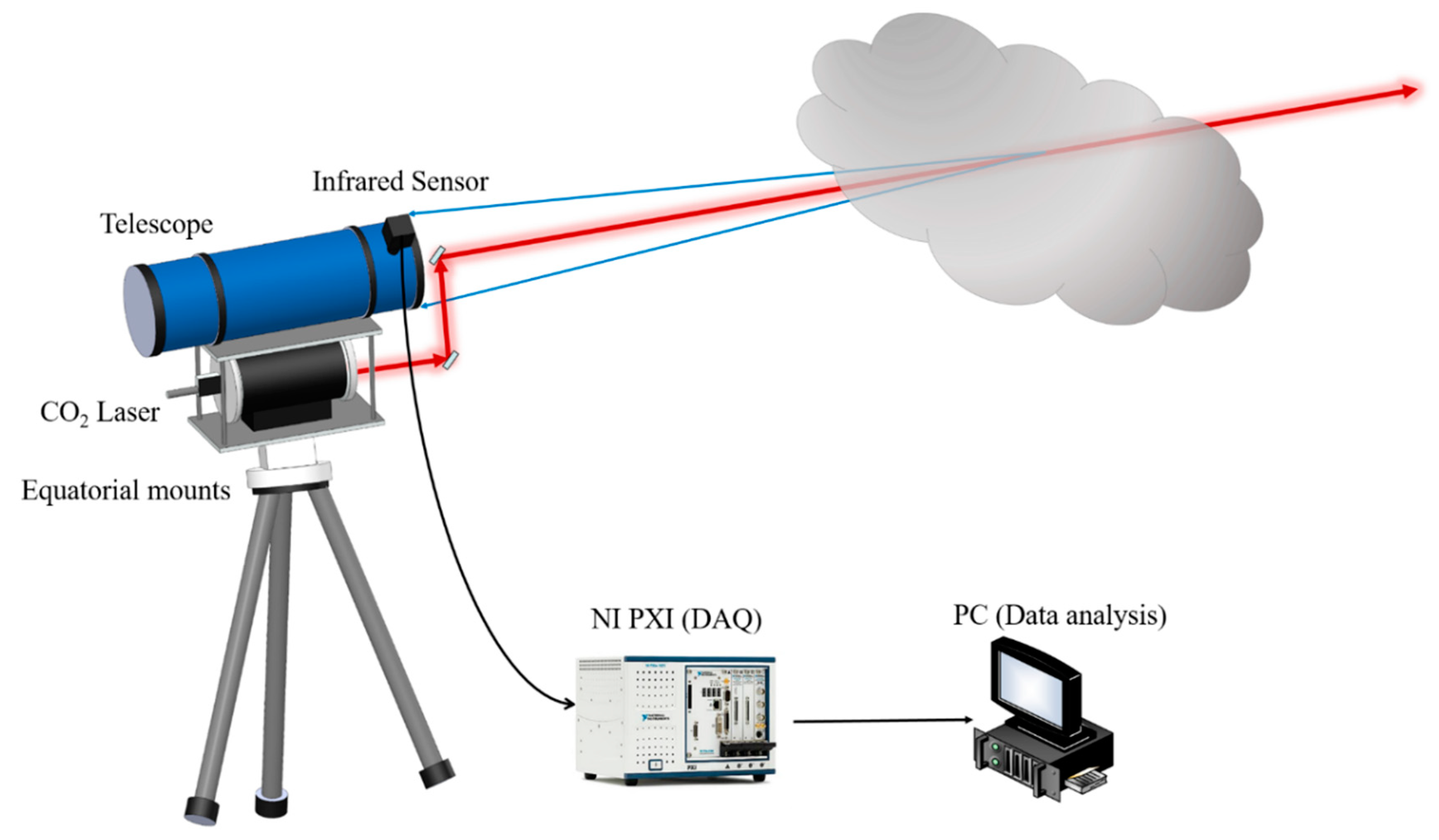
The measurements were performed by a mini dial system TELEMACO based on a tunable CO2 laser (MTL-5 mini TEA CO₂) operating between 9.9 μm and 11 μm wavelengths (about 60 different laser lines). The laser pulse width was 50 ns and the maximum repetition rate was 200 Hz. The laser was tuned by a step-motor (Mercury™ II DC-Motor Controller/Driver) connected to the laser grating. The backscattered light was acquired by the Newtonian telescope (model Ziel GALAXY 2), which collects the light and sends it to an infrared sensor. The telescope diameter was 200 mm and the focal length was 1000 mm. The detector was an MCT that converts the light signal in an electrical one, which was collected by the Data Acquisition System, a National Instrument (NI) PXI. The PXI was equipped with three NI cards (NI PXI-5122, NI PXI-6509 and NI PXI-7330). They allow providing all the input/output signals to control the experiment. The data acquisition frequency was 100 megasamples/s. Equatorial mounts allow to direct the laser beam and perform areal or volumetric measurements. Figure 1 shows a schematic representation of the experimental apparatus.

The apparatus works as follows:

• Wavelength tuning: the step motor tunes the grating to select the proper wavelength;
• The laser performs N shots (chosen by the user, in this work was 100) and each shot was acquired by the DAQ;

The two steps are repeated for each wavelength to measure. The data were stored in the PXI. A computer was Wi-fi connected to the PXI and iteratively downloads the measured signals and perform the analysis.

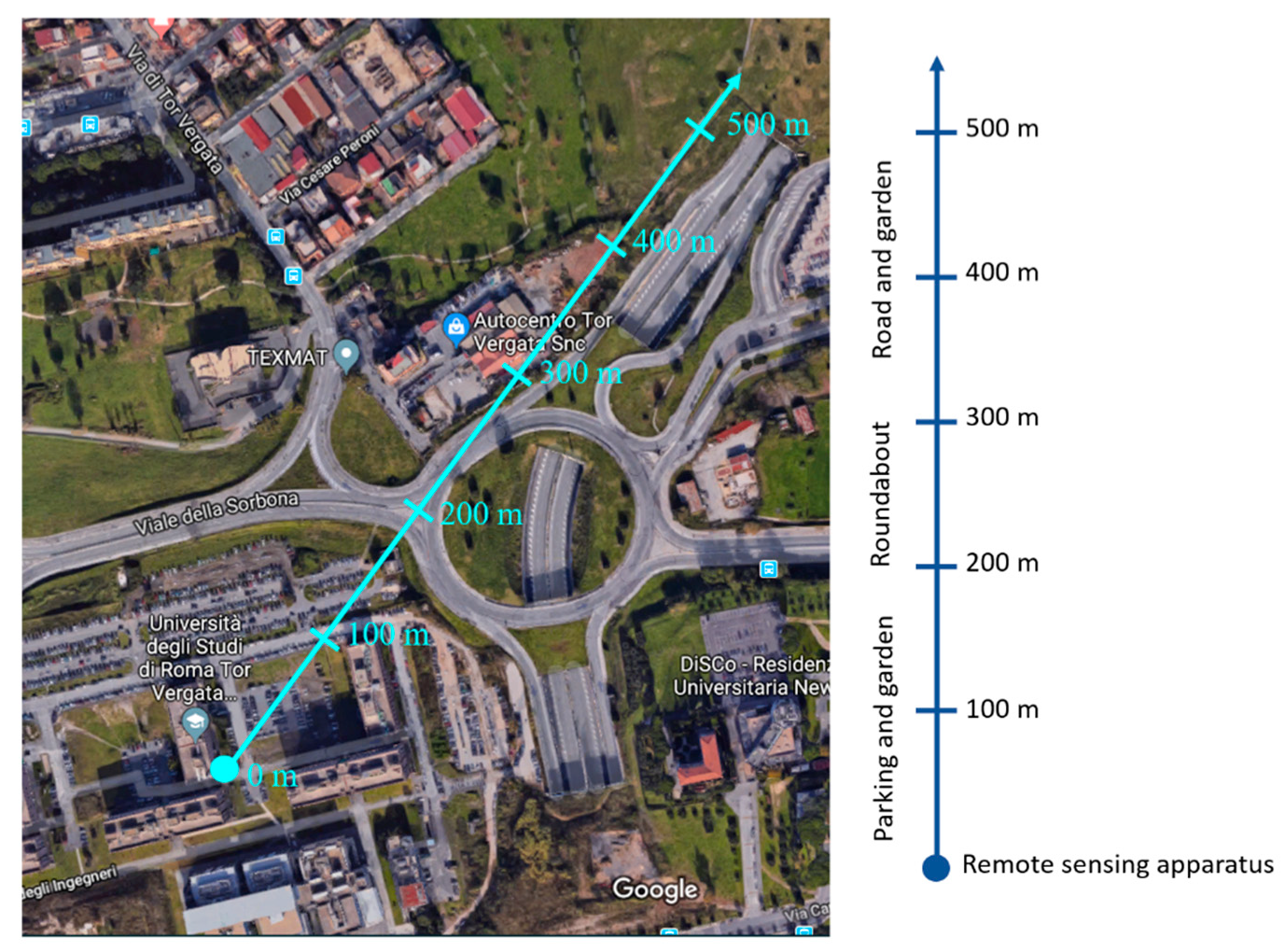
The preliminary measurements were made at the University of Rome Tor Vergata Campus. The system was located in the laboratories of Quantum Electronics and Plasma Physics research group (QEP, www.qepresearch.it) at the Department of Industrial Engineering and the measurements were performed along a specific line, shown in Figure 2. The line of sight crosses a highly trafficked roundabout. The measurements were performed during a working day, from 11:00 to the 16:00.

Before the signal processing through the classic dial or the LSM dial equation, the lidar signals were filtered by a moving average filter. The LSM dial was performed in different ways. In the case of water, a two-wavelength LSM dial with only the water vapor concentration unknown was performed. Thus, the matrices of the LSM equation are written as follows:

$$\Lambda =\left[\begin{array}{c}{\sigma }_{H2O,10R18}\\ {\sigma }_{H2O,10R20}\end{array}\right];U=N_{H2O};\Theta =\left[\begin{array}{c}\frac{1}{2}\frac{d}{dr}\left[\ln \left(P_{10R18}\left(r\right)r^2\right)\right]\\ \frac{1}{2}\frac{d}{dr}\left[\ln \left(P_{10R20}\left(r\right)r^2\right)\right]\end{array}\right]$$

(17)

A two-wavelength LSM, adding the ammonia concentration as unknown, was tried. However, since the ammonia has a much smaller differential cross-section (

Table 1. Optical properties at the three wavelengths.

	10R08	10R10	10R12
σNH3 [m−1 atm−1]	142.3	326.2	1647
σH2O [m−1 atm−1]	2.99 × 10−3	4.76 × 10−4	2.56 × 10−3
f [a.u.]	1	0.9942	0.9884

) and concentration respect with the water vapor, its influence is negligible and does not affect the result. The matrices, in this case, are written as follows:

$$\Lambda =\left[\begin{array}{c}{\sigma }_{H2O,10R18}\\ {\sigma }_{H2O,10R20}\end{array}\right];U=N_{H2O};\Theta =\left[\begin{array}{c}\frac{1}{2}\frac{d}{dr}\left[\ln \left(P_{10R18}\left(r\right)r^2\right)\right]\\ \frac{1}{2}\frac{d}{dr}\left[\ln \left(P_{10R20}\left(r\right)r^2\right)\right]\end{array}\right]$$

(18)

The proper measurements of ammonia are performed with a three-wavelength LSM, introducing the extinction coefficient unknown and the system of equations becomes:

$$\Lambda =\left[\begin{array}{cc}\begin{array}{c}\begin{array}{c}{\sigma }_{NH3,10R08}\\ {\sigma }_{NH3,10R10}\end{array}\\ {\sigma }_{NH3,10R12}\end{array}& \begin{array}{cc}\begin{array}{c}\begin{array}{c}{\sigma }_{H2O,10R08}\\ {\sigma }_{H2O,10R10}\end{array}\\ {\sigma }_{H2O,10R12}\end{array}& \begin{array}{c}{f}_1\\ f_2\\ f_3\end{array}\end{array}\end{array}\right];U=\left[\begin{array}{c}{N}_{NH3}\\ \begin{array}{c}{N}_{H2O}\\ k\end{array}\end{array}\right];\Theta =\left[\begin{array}{c}\begin{array}{c}\frac{1}{2}\frac{d}{dr}\left[\ln \left(P_{10R08}\left(r\right)r^2\right)\right]\\ \frac{1}{2}\frac{d}{dr}\left[\ln \left(P_{10R10}\left(r\right)r^2\right)\right]\end{array}\\ \frac{1}{2}\frac{d}{dr}\left[\ln \left(P_{10R12}\left(r\right)r^2\right)\right]\end{array}\right]$$

(19)

4. Results

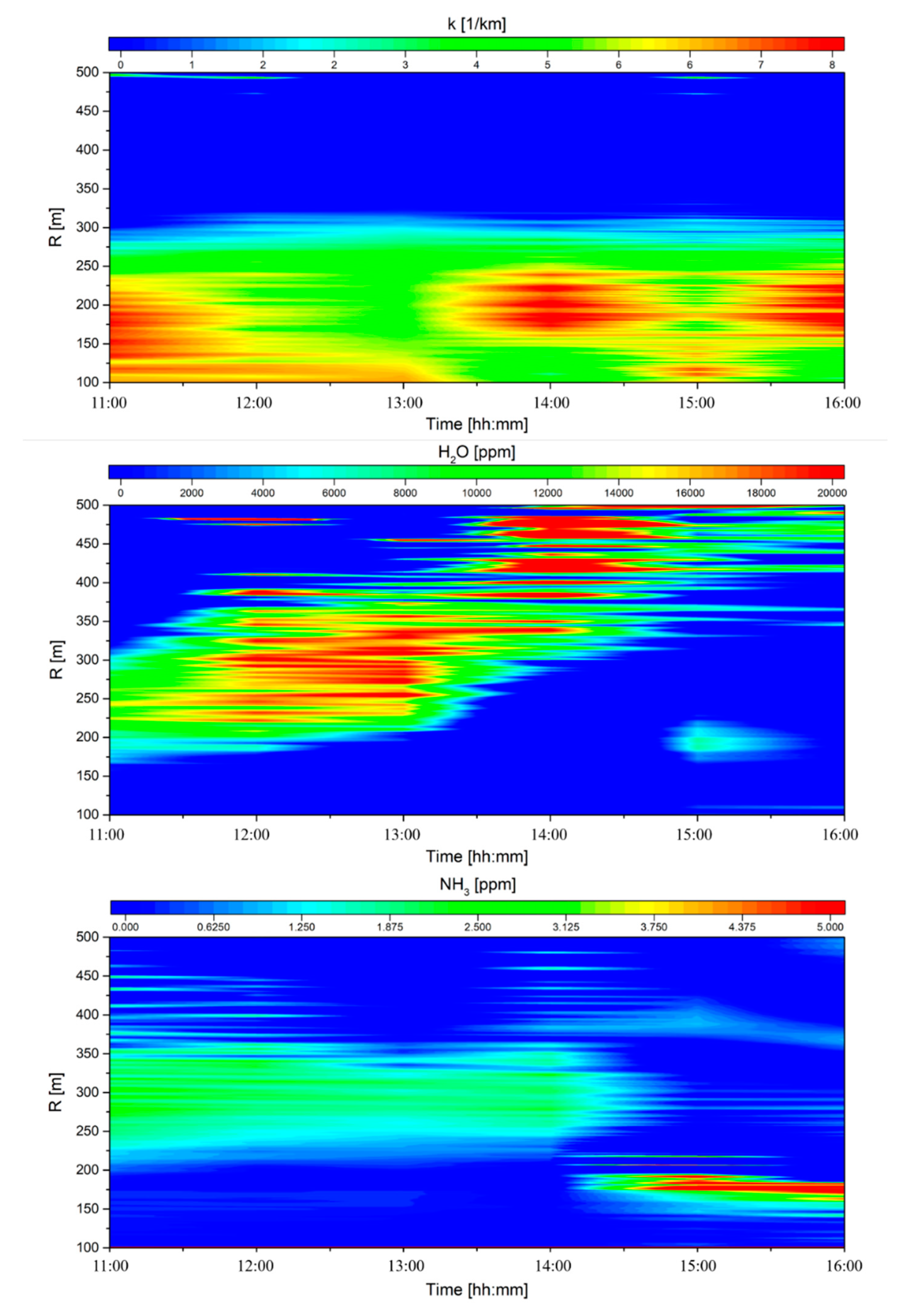
Figure 3 shows the extinction coefficient and the maps of the concentration of water vapor and ammonia as a function of the distance and the time. The extinction coefficient, measured by Equation (19) showed a large value from 100 m to 250 m, while it decreased to very small value after 300 m. This tendency was observed at any time. The large values of the extinction coefficient—which were usually observed in clouds—indicate that over the roundabout there was a large extinction of the light in the infrared region, probably due to the emissions of greenhouses gases and other chemicals. The high and unexpected decrease of the extinction coefficient after 300 m was probably due to the large absorbance and scattering of the radiation, which involved a large decrease of the backscattered signal and a consequent increase of the measurement noise and uncertainty.

The second map shows the concentration of water vapor, which was, together with CO₂, the major product of the combustion process [29]. A large increase of the water vapor concentration was observed in the region which goes from 200 m to 350 m, exactly over the roundabout, where the highest concentration due to traffic was expected in absence of the wind. From 14:00 to 16:00, the water vapor peaks were recorded in a region which goes from 350 m to 500 m. This shift may be due to the wind, which has displaced the plume. In some regions, negative or zero water vapor concentration was measured. These values, obviously wrong, were probably due to the small sensitivity of dial to water vapor concentration—even small noise made the measurement erroneous where the water concentration was not high.

The last map shows the concentration of ammonia, which follows the water vapor concentration. From 11:00 to 14:00, the highest value of ammonia concentration was recorded over the roundabout (from 200 m to 350 m). After 14:00, some peaks of ammonia concentration, even if smaller, were recorded from 350 m to 500 m. The smaller value may be related to the wind, which displacing the pollution plume also diffuses it, diluting the chemicals in a larger volume. A very high level of ammonia concentration was also recorded in the range 120—200 m, which was also linked with an increase of the water vapor concentration. Different possibilities may be linked to this increase detected for both ammonia and water vapor:

• In the range 120—200 m there was the parking of the university, thus the peaks may be due to emissions of the car in this area;
• Near the parking there was also a small garden, which may be watered and fertilized;
• Other sources of pollutions.

It was not possible to validate these measures with a comparison of data coming from different instruments. The alternative was a comparison of the measures with the expected values to produce a coherent interpretation of the results.

Moreover, correlating independent measurements may help in providing a critical analysis.

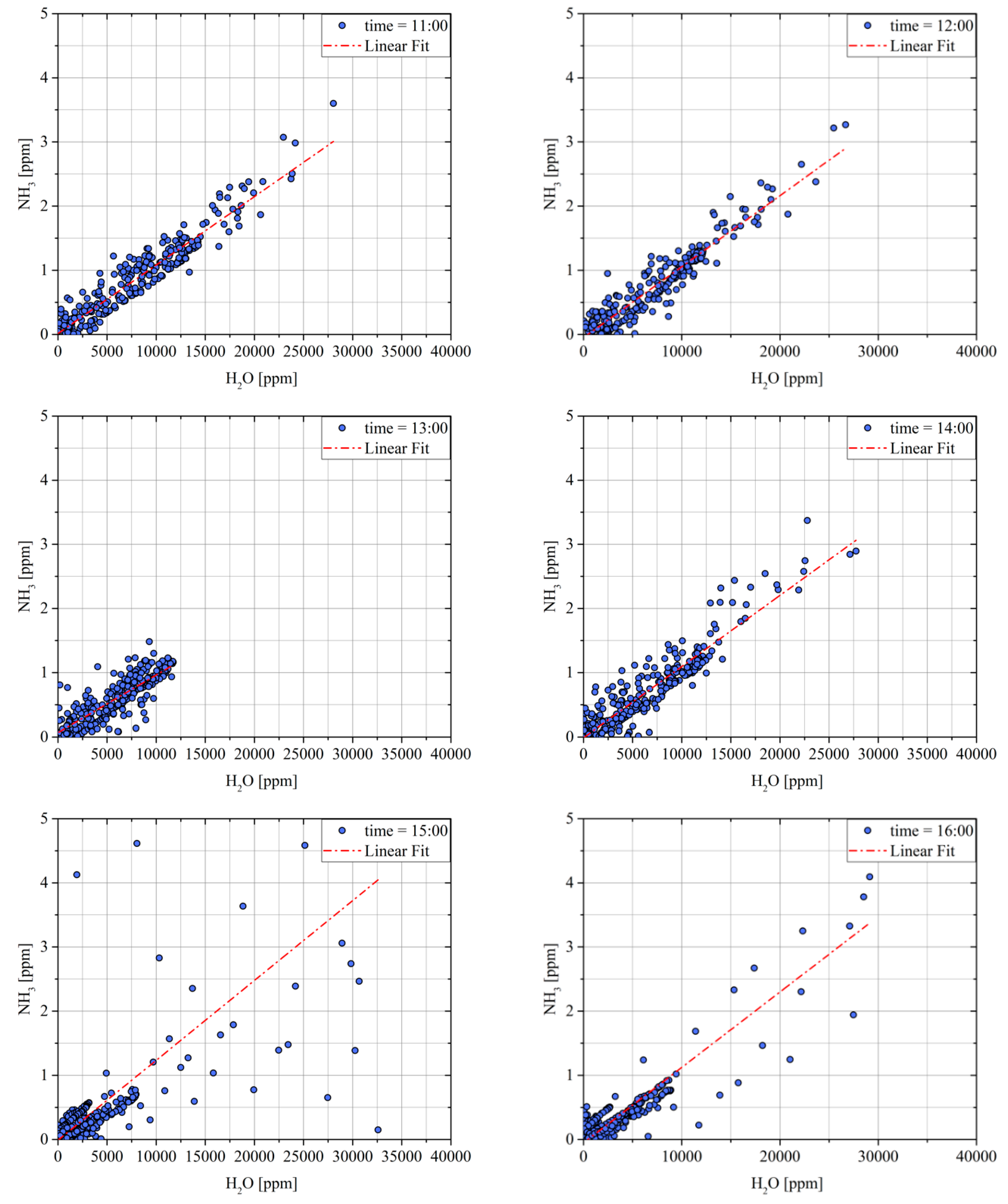
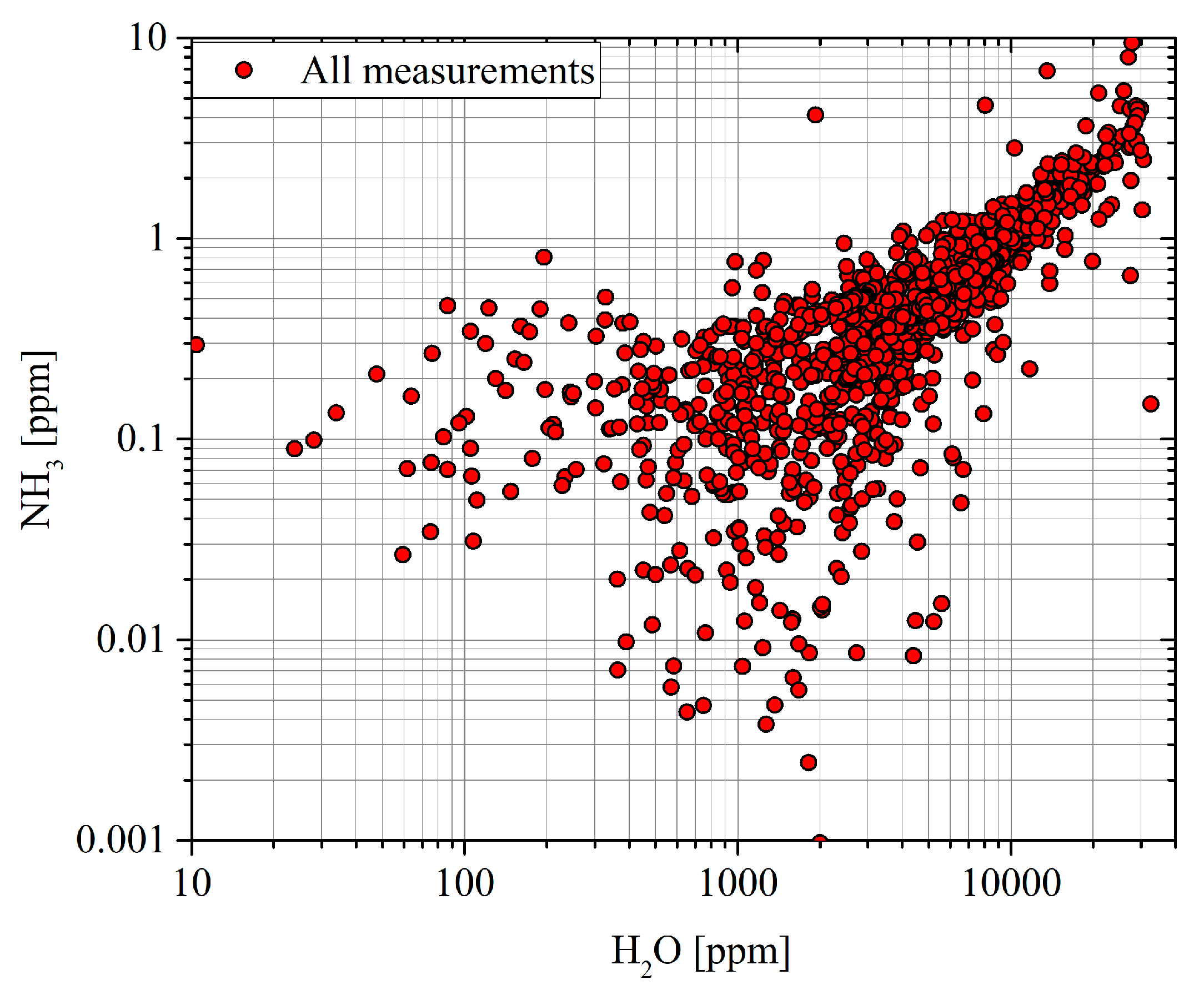
In the specific case, both the water vapor and the ammonia concentrations were measured by a dial system over a high traffic area, where it was expected that the chemical concentration was dominated by the traffic. Both water vapor and ammonia are emitted as exhaust gases from the cars and an increase in the water vapor concentration should correspond to an increase in the ammonia concentration. Moreover, this correlation should be linear, since both concentrations should be related to the number of vehicles. Supposing a car which that emits an average quantity of water, called c_H2O, and an average quantity of ammonia, called c_NH3, the correlation of the measurements should have a slope of c_NH3/c_H2O. Even if the correlation were much more complex, depending on many other unpredictable factors (car velocity, motor type, duty cycle, etc.), this simple approximation should not lead to large discrepancies from the reality.

Figure 4 shows the correlation between water vapor and ammonia concentration measured at six different times (11:00, 12:00, 13:00, 14:00, 15:00 and 16:00), while Figure 5 shows the correlation considering all the measurements together. All the graphs show a clear correlation between the two chemical concentrations, which have also similar slopes in all cases, as reported in

Table 2. Slope and corrected R2 of the linear correlation between ammonia and water vapor concentration.

Time [hh:mm]	11:00	12:00	13:00	14:00	15:00	16:00
Slope	0.000107	0.000111	0.0000897	0.000111	0.000124	0.000118
R2	0.896	0.898	0.668	0.848	0.482	0.840

. Figure 5 shows the correlations in the logarithm scale and another issue must be highlighted: the correlation was high for large values of both concentrations, while it was very low for the smallest measured values. This circumstance was justified by two facts:

• Noise becomes dominant at low concentrations;
• The correlation of ammonia and water vapor should be smaller far from the roundabout, where the ammonia and water vapor concentrations depend by other sources, many independents (water evaporation from surfaces, garden irrigation and fertilization, etc.).

Considered the measurements validated, the values of the extinction coefficient, the ammonia and water vapor concentrations clearly showed that over a high traffic area, the pollutant concentration may reach very large values. The extinction ratio in the infrared region reaches very high values, which were normally achieved only in dense media, such as clouds, which was expected since the many exhaust gases are greenhouse gases. Water vapor increases as well and, even if water vapor is not dangerous, its measurement may be performed to estimate the concentration of other gases, knowing the average emissions of vehicles, as demonstrated with the ammonia concentration.

5. Conclusions

This work aims to demonstrate the applicability of the differential absorption lidar for the measurement of pollutant concentrations in high traffic areas, taking as a case study a roundabout near the Laboratory of QEP research group at the Department of Industrial Engineering of the University of Rome Tor Vergata. The atmospheric extinction coefficient, the water vapor and the ammonia concentration were measured. The ammonia concentration and the extinction coefficient were measured through a multiwavelength approach, in order to decrease the influence of water vapor in these measurements, which previous works have demonstrated to be one of the highest sources of uncertainty in differential absorption measurements.

The experimental measurements shown in this work were performed in a complex environment, considering that the measurement of pollution plume emitted by many vehicles is one of the hardest dial challenges. First, there is a large variety of exhaust gases. Water vapor and carbon dioxide are the direct products of the combustion, but many other chemicals are emitted, such as nitrogen oxides, sulfur oxides, ozone and ammonia. Furthermore, particulate matters are also emitted, and they involve a strong variation of the scattering coefficient and so of the extinction coefficient. Due to the variety of combustion technologies, fuels, filters and driving conditions, the correlation between those gases vary as well; it is not possible to determine a general law. Moreover, the weather conditions and the local turbulence of the atmosphere play a fundamental role, especially the wind which determines the plume shift as a function of the time, its shape and the speed of concentration variability of the plume.

All these issues make the dial measurement hard to be performed. First of all, because the homogeneous atmosphere hypothesis is not allowed. Furthermore, the extinction coefficients vary as a function of the pollution intensity and the hypothesis of an exponential correlation between the extinction coefficient and the wavelength may fall, especially if the molecular scattering and absorption are larger than the particle scattering. A considerable increase of the apparatus performances may be obtained increasing the number of wavelengths and the number of unknowns measured (an increase of the measured variables implies a decrease of the assumptions). However, the speed of concentration variability requires that all the backscattered signals are measured in a time smaller than the time constant of the plume variability. Thus, the best option to guarantee an accurate measurement of a pollution plume is a multiwavelength measurement by a multi-laser system and not a single tunable laser. However, this solution requires larger costs.

The value maps as a function of the time and the distance were calculated for the three measured variables, and it was observed a very large increase of the pollutants exactly above the roundabout. To have a validation of the measurements, the water vapor and the ammonia concentrations, which were measured by different dial signals, were performed. Above a traffic area, a good correlation between the exhaust gases is expected. The correlation analysis showed that water vapor and ammonia were highly correlated, confirming that both gases become from the same source (vehicles).

It has to be noted that the concentration of ammonia is quite large and unexpected. It may be due to the influence of other pollutants, which have not been considered in the dial equation, but which may involve an overestimation (or underestimation) of the measured values. From a theoretical point of view, this problem may be solved just adding other terms in the LSM dial equations. However, it needs also other dial signals, which must be measured with very short time delays, not possible with the actual experimental apparatus configuration. However, the high concentration of greenhouse gases—observed by the high infrared extinction coefficient, the high-water vapor and ammonia concentrations—demonstrated that the differential absorption lidar is a good candidate to monitor the atmosphere quality and detect high polluted areas.