Assessment of a Coastal Offshore Wind Climate by Means of Mesoscale Model Simulations Considering High-Resolution Land Use and Sea Surface Temperature Data Sets


Abstract
1. Introduction
2. Numerical Model and Field Measurement
2.1. Numerical Model
2.2. Field Measurement
3. The Effect of Nudging Scheme, Land-Use and Sea Surface Temperature on the Wind Prediction
3.1. The Effect of Nudging Scheme
3.2. The Effect of Land-Use
3.3. The Effect of Sea Surface Temperature
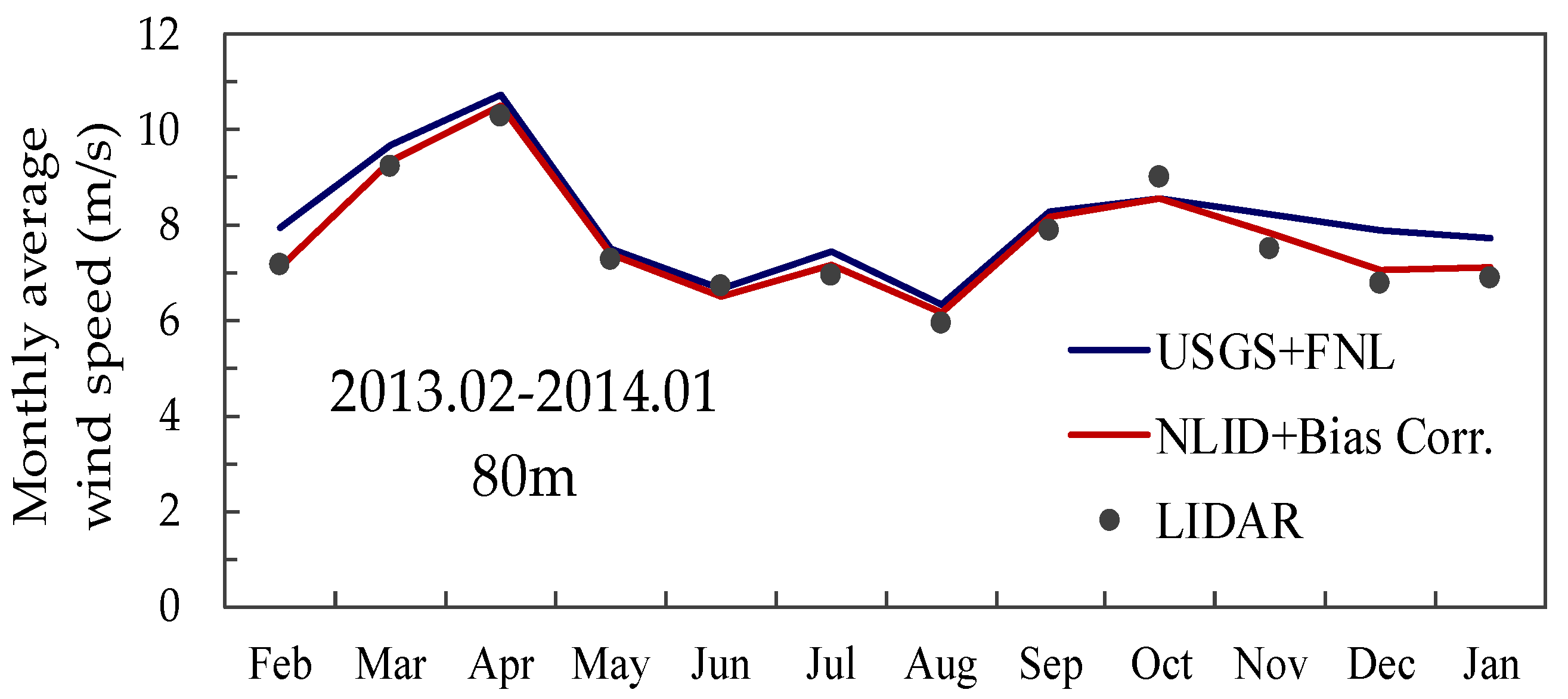
3.4. Evaluation of Predicted Annual and Seasonal Average Wind Speed
4. Conclusions
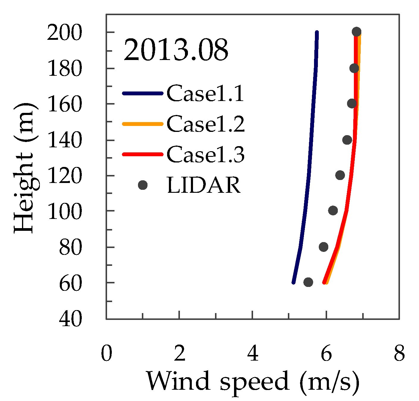
- When the nudging is applied to full levels in the outer domain and to the levels above the planetary boundary layer in the domains, the local wind is reproduced and the phase error is suppressed at the same time.
- The land-use datasets are created from a higher-resolution land-use data by using the maximum area sampling scheme according to the horizontal resolution of the mesoscale model. The high-resolution land-use data improves the overestimation of the northerly wind from the Choshi area.
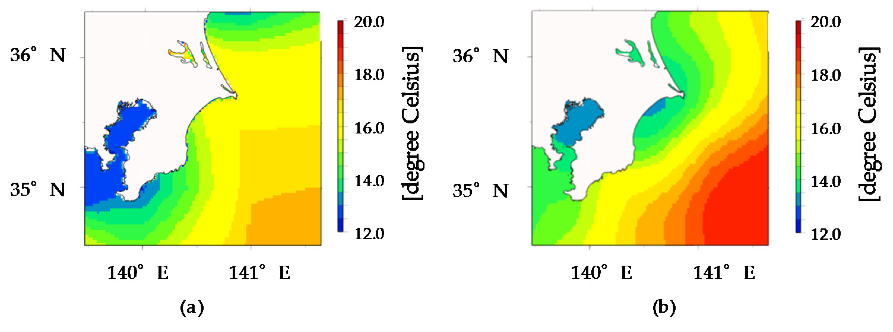
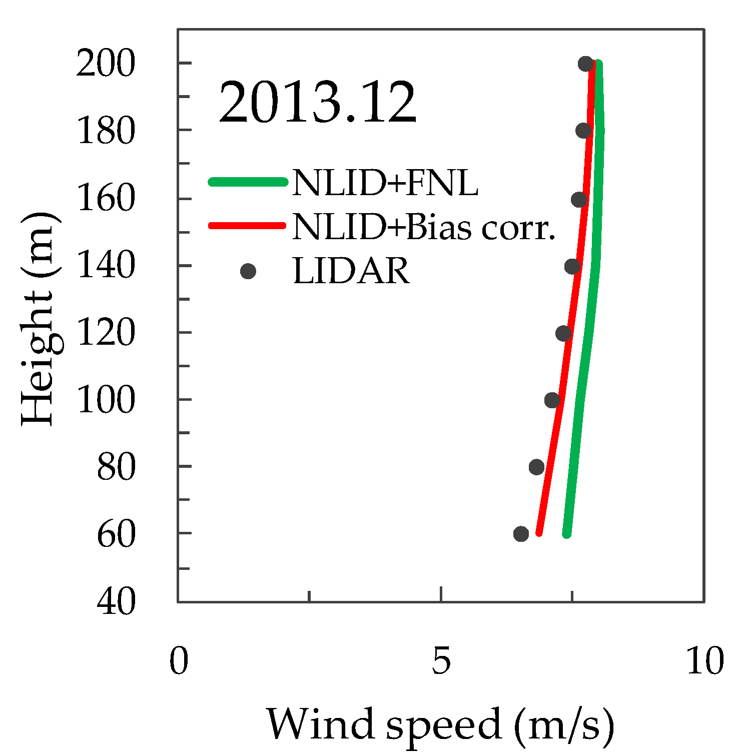
- The bias-correction method for the sea surface temperature is proposed by using the onsite observation data. The bias-corrected sea surface temperature suppresses the convection in the winter season and improves the overestimation of annual average wind speed in the south-western direction.
- The relative error of annual average wind speed at the hub height reduces from 7.3% to 2.2% and the correlation factor of wind speed improves from 0.80 to 0.84 by using the high-resolution land-use data and bias-corrected sea surface temperature in the coastal region. The 1% relative error is reduced by using high-resolution land-use data and 4.1% is reduced by using the bias-corrected SST data.
Author Contributions
Acknowledgments
Conflicts of Interest
References
- FINO1-Research Platform in the North and Baltic Seas No.1. Available online: https://www.fino1.de/en/about-fino1.html (accessed on 4 April 2020).
- FINO2-Reseach Platform in the Baltic Sea. Available online: https://www.fino2.de/en/ (accessed on 4 April 2020).
- FINO3-Reseach Platform in the North Sea and the Baltic No.3. Available online: https://www.fino3.de/en/ (accessed on 4 April 2020).
- Meteomast IJmuiden. Available online: https://www.windopzee.net/en/locations/meteomast-ijmuiden-mmij/ (accessed on 4 April 2020).
- New Energy and Industrial Technology Development Organization (NEDO), Offshore Observation Facility Open Data. Available online: http://www.nedo.go.jp/fuusha/public/index.html (accessed on 4 April 2020).
- Yamaguchi, A.; Ishihara, T. A new motion compensation algorithm of floating lidar system for the assessment of turbulence intensity. J. Phys. Conf. Ser. 2016, 753, 072034. [Google Scholar] [CrossRef]
- Kelberlau, F.; Neshaug, V.; Lonseth, L.; Bracchi, T.; Mann, J. Taking the motion out of floating lidar: Turbulence intensity estimates with a continuous-wave wind lidar. Remote Sens. 2020, 12, 898. [Google Scholar] [CrossRef]
- Skamarock, W.; Klemp, J.; Dudhia, J.; Gill, D.; Barker, D.; Duda, M.; Huang, X.; Wang, W.; Powers, J. A Description of the Advanced Research WRF Version 3; (No. NCAR/TN-475+ STR); University Corporation for Atmospheric Research: Boulder, Colorado, USA, 2008. [Google Scholar] [CrossRef]
- Berge, E.; Byrkjedal, Ø.; Ydersbond, O.; Kindler, D. Modeling of offshore wind resources. Comparison of meso-scale model and measurements from FINO-1 and North Sea oil rigs. In Proceedings of the European Wind Energy Conference 2009, Marseille, France, 16–19 March 2009. [Google Scholar]
- Hahmann, A.N.; Vincent, C.L.; Pena, A.; Lange, J.; Hasager, C.B. Wind climate estimation using WRF model output: Method and model sensitivities over the sea. Int. J. Climatol. 2015, 35, 3422–3439. [Google Scholar] [CrossRef]
- Fukushima, M.; Yamaguchi, A.; Ishihara, T. Offshore wind speed prediction by using mesoscale model. In Proceedings of the Grand Renewable Energy 2014, Yokohama, Japan, 27 July–1 August 2014. [Google Scholar]
- Ishihara, T.; Yamaguchi, A.; Goit, J.; Tanemoto, J. Validation of numerical weather simulation by using 3D scanning lidar. J. Wind Eng. 2017, 42, 87–88. (In Japanese) [Google Scholar] [CrossRef]
- Lopez-Espinoza, E.D.; Zavala-Hidalgo, J.; Gomez-Ramos, O. Weather forecast sensitivity to changes in urban land covers using the WRF Model for central Mexico. Atmósfera 2012, 25, 127–154. [Google Scholar]
- Cheng, F.Y.; Hsu, Y.C.; Lin, P.L.; Lin, T.H. Investigation of the effects of different land use and land cover patterns on mesoscale meteorological simulations in the Taiwan area. J. Appl. Meteor. Climatol. 2013, 52, 570–587. [Google Scholar] [CrossRef]
- Li, D.; Bou-Zeid, E.; Baeck, M.; Jessup, S.; Smith, J. Modeling land surface processes and heavy rainfall in urban environments: Sensitivity to urban surface representations. J. Hydrometeor. 2013, 14, 1098–1118. [Google Scholar] [CrossRef]
- Kamal, S.; Huang, H.-P.; Myint, S.W. The influence of urbanization on the climate of the Las Vegas metropolitan area: A numerical study. J. Appl. Meteor. Climatol. 2015, 54, 2157–2177. [Google Scholar] [CrossRef]
- Mallard, M.S.; Spero, T.L.; Taylor, S.M. Examining WRF’s sensitivity to contemporary land-use datasets across the contiguous United States Using Dynamical Downscaling. J. Appl. Meteor. Climatol. 2018, 57, 2561–2583. [Google Scholar] [CrossRef]
- Yoshie, R.; Mirura, S. Preparation of standard wind data for assessment of pedestrian wind environment using WRF. J. Wind Eng. 2014, 39, 154–159. (In Japanese) [Google Scholar] [CrossRef][Green Version]
- Shimada, S.; Osawa, T.; Kogaki, T.; Steinfeld, G.; Heinemann, D. Effects of sea surface temperature accuracy on offshore wind resource assessment using a mesoscale model. Wind Energy 2015, 18, 1839–1854. [Google Scholar] [CrossRef]
- Donlon, C.J.; Martin, M.; Stark, J.; Roberts-Jones, J.; Fiedler, E.; Wimmer, W. The operational sea surface temperature and sea ice analysis (OSTIA). Remote Sens. Environ. 2012, 116, 140–148. [Google Scholar] [CrossRef]
- NOAA Earth System Research Laboratory, NCEP Reanalysis Data Provided by the NOAA/OAR/ESRL PSD, Boulder, Colorado, USA. Available online: http://www.esrl.noaa.gov/psd/ (accessed on 4 April 2020).
- Witha, B.; Hahmann, A.; Sile, T.; Dorenkamper, M.; Ezber, Y.; Garcia-Bustamante, E.; Gonzalez-Rouco, J.F.; Leroy, G.; Navarro, J. WRF model sensitivity studies and specifications for the NEWA mesoscale wind atlas production runs. New Eur. Wind Atlas Deliv. 2019, 4. [Google Scholar]
- Stauffer, D.R.; Seaman, N.L.; Binkowski, F.S. Use of Four-Dimensional Data Assimilation in a Limited-Area Mesoscale Model Part II: Effects of Data Assimilation within the Planetary Boundary Layer. Mon. Wea. Rev. 1991, 119, 734–754. [Google Scholar] [CrossRef]
- Stauffer, D.R.; Seaman, N.L.; Binkowski, F.S. Use of Four-Dimensional Data Assimilation in a Limited-Area Mesoscale Model Part I: Experiments with Synoptic-Scale Data. Mon. Wea. Rev. 1990, 118, 1250–1277. [Google Scholar] [CrossRef]
- Vincent, C.L.; Hahmann, A. The impact of grid and spectral nudging on the variance of the near-surface wind speed. J. Appl. Meteor. Clim. 2015, 54, 1021–1038. [Google Scholar] [CrossRef]
- Misaki, T.; Ohsawa, T.; Konagaya, M.; Shimada, S.; Takeyama, Y.; Nakamura, S. Accuracy comparison of coastal wind speeds between WRF simulations using different input datasets in Japan. Energies 2019, 12. [Google Scholar] [CrossRef]
- U.S. Geological Survey. Land Use Land Cover Modeling. Available online: https://www.usgs.gov/land-resources/eros/lulc/data-tools (accessed on 4 April 2020).
- Geospatial Information Authority of Japan, GSI Web Site. Available online: https://www.gsi.go.jp/ENGLISH/page_e30233.html (accessed on 4 April 2020).
- National Spatial Planning and Regional Policy Bureau of Japan, Land Use Tertiary Mesh Data. Available online: http://nlftp.mlit.go.jp/ksj-e/gml/datalist/KsjTmplt-L03-a.html (accessed on 4 April 2020).
- Yoshie, R.; Miura, S.; Mochizuki, M. Validation of WRF for preparation of standard wind data for assessment of pedestrian wind environment. J. Wind Eng. 2015, 40, 113–122. (In Japanese) [Google Scholar] [CrossRef]
- Cressman, G.P. An operational objective analysis system. Mon. Wea. Rev. 1959, 87, 367–374. [Google Scholar] [CrossRef]
- Sathe, A.; Grying, S.; Pena, A. Comparison of the atmospheric stability and wind profiles at two wind farm sites over a long marine fetch in the North Sea. Wind Energy 2011, 14, 767–780. [Google Scholar] [CrossRef]


| Domain 1 | Domain 2 | Domain 3 | |
|---|---|---|---|
| Simulation period | February 2013–January 2014 | ||
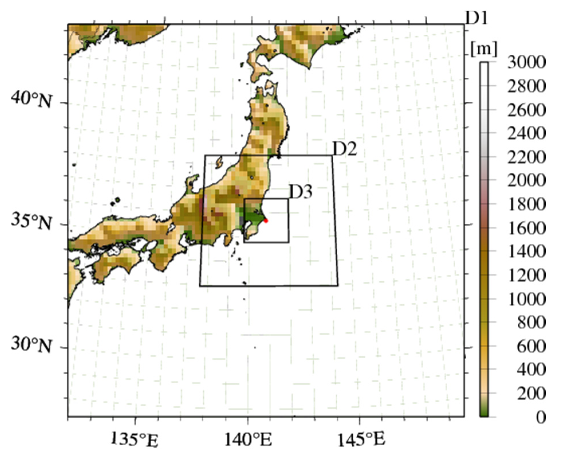
| Domain | 133o–149o E, 28.0o–44.0o N | 138.5o–142.5o E, 33.5o–37.5o N | 139.7o–141.3o E, 34.7o–36.3o N |
| Horizontal resolution | 18 km (100 × 100 grids) | 6 km (100 × 100 grids) | 2 km (100 × 100 grids) |
| Vertical resolution | 45 levels (Surface to 50 hPa) | ||
| Time step | 72 sec. | 24 sec. | 8 sec. |
| Spin-up | One month | ||
| Boundary condition | NCEP-FNL 1o × 1o 6-hourly | ||
| Physics option | Ferrier (new Eta) microphysics scheme | ||
| Rapid radiative transfer model | |||
| Dudhia scheme | |||
| Monin-Obukhov (Janjic Eta) scheme | |||
| Unified Noah land surface model | |||
| Mellor-Yamada-Janjic (Eta) TKE level 2.5 scheme | |||
| Betts-Miller-Janic scheme (Except for domain 3) | |||
| Nudging | Described in Section 3.1 | ||
| Land use | Described in Section 3.2 | ||
| Sea surface temperature | Described in Section 3.3 | ||
| Equipment | Height | Sampling Rate |
|---|---|---|
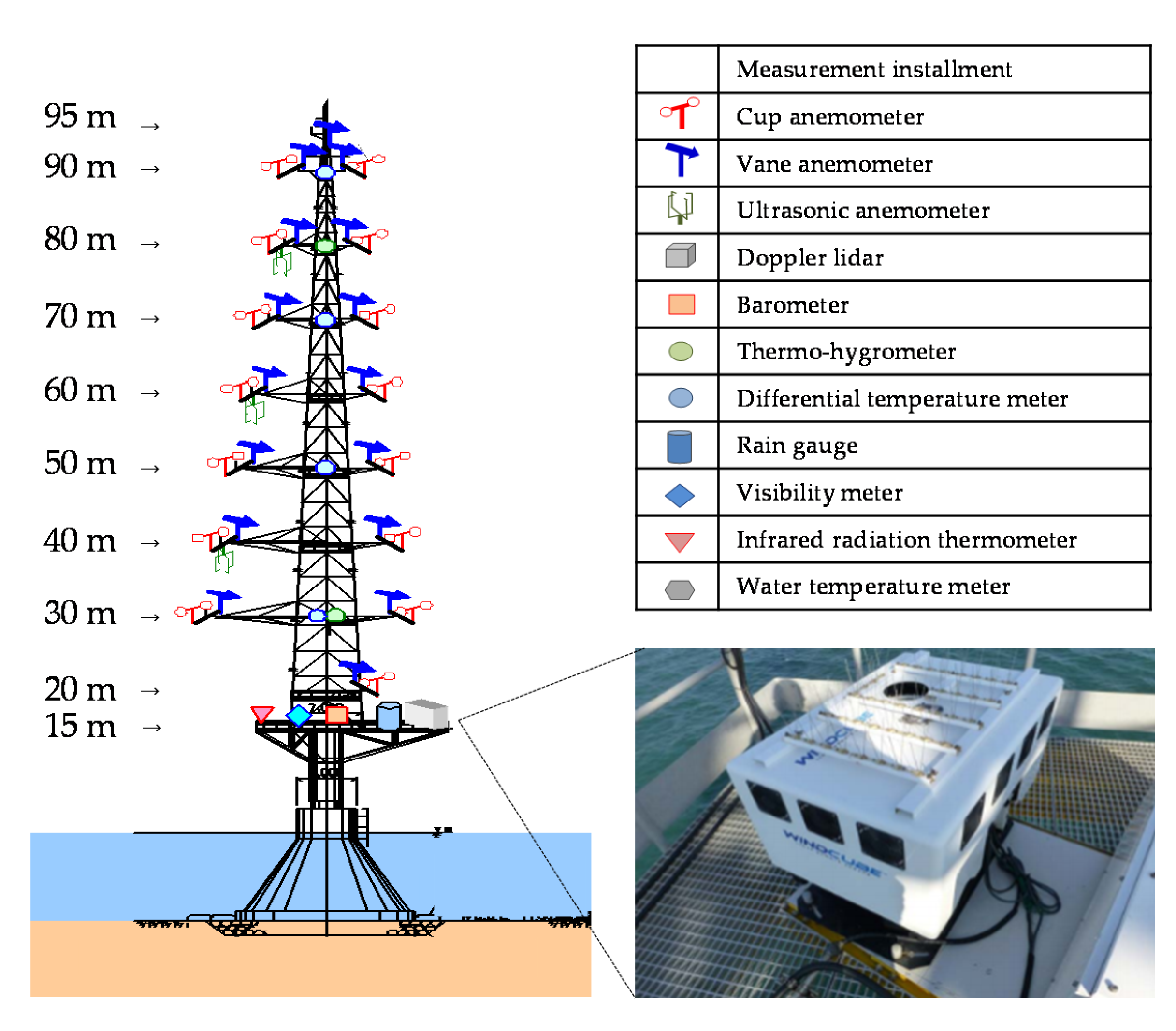
| Cup anemometer | 8 heights (20 m–90 m, 10 m interval) | 4 Hz |
| Vane anemometer | 9 heights (20–90 m, 10 m interval, 95 m) | 4 Hz |
| Ultrasonic anemometer | 3 heights (40, 60, 80 m) | 20 Hz |
| Doppler lidar | 8 heights (60–200 m, 20 m interval) | 4 Hz |
| Water temperature meter | 3 heights (T.P. 0 m, −1 m, −2 m) | 4 Hz |
| Barometer | 1 height (Platform) | 4 Hz |
| Thermo-hygrometer | 2 heights (30 m, 80 m) | 4 Hz |
| Differential temperature meter | 4 heights (30–90 m, 20 m interval) | 4 Hz |
| Case | Domain | |||
|---|---|---|---|---|
| 1 | 2 | 3 | ||
| Case 1.1 | Above PBL | ○ | ○ | ○ |
| Below PBL | ○ | ○ | ○ | |
| Case 1.2 | Above PBL | ○ | ○ | ○ |
| Below PBL | × | × | × | |
| Case 1.3 | Above PBL | ○ | ○ | ○ |
| Below PBL | ○ | × | × | |
| Case | Land-Use | SST |
|---|---|---|
| Case 2.1 | USGS | OSTIA |
| Case 2.2 | NLID | OSTIA |
| Case | Land-Use | Sea Surface Temperature | Onsite Observation Data |
|---|---|---|---|
| Case 3.1 | NLID | FNL | Without Choshi observation data |
| Case 3.2 | NLID | OSTIA | With Choshi observation data |
| Case | Land-Use | Sea Surface Temperature | Relative Error | Correction Factor |
|---|---|---|---|---|
| Case 4.1 | USGS | FNL | 7.3% | 0.80 |
| Case 4.2 | NLID | Bias corrected OSTIA | 2.2% | 0.84 |
| Land-use Data | Sea Surface Temperature | Relative Error | Correlation | |||
|---|---|---|---|---|---|---|
| USGS | NLID | FNL | OSTIA | Bias Correction | ||
| ○ | □ | 7.3% | 0.80 | |||
| ● | □ | 6.3% | ||||
| ○ | ■ | 5.6% | ||||
| ● | ■ | 4.2% | ||||
| ● | ■ | ▲ | 2.2% | 0.84 | ||
| Atmospheric Stability Category | Monin-Obukhov Length |
|---|---|
| Very stable | 10 < L < 50 |
| Stable | 50 < L < 200 |
| Neutral | |L| > 200 |
| Unstable | −200 < L < −100 |
| Very unstable | −100 < L < −50 |
© 2020 by the authors. Licensee MDPI, Basel, Switzerland. This article is an open access article distributed under the terms and conditions of the Creative Commons Attribution (CC BY) license (http://creativecommons.org/licenses/by/4.0/).
Share and Cite
Kikuchi, Y.; Fukushima, M.; Ishihara, T. Assessment of a Coastal Offshore Wind Climate by Means of Mesoscale Model Simulations Considering High-Resolution Land Use and Sea Surface Temperature Data Sets. Atmosphere 2020, 11, 379. https://doi.org/10.3390/atmos11040379
Kikuchi Y, Fukushima M, Ishihara T. Assessment of a Coastal Offshore Wind Climate by Means of Mesoscale Model Simulations Considering High-Resolution Land Use and Sea Surface Temperature Data Sets. Atmosphere. 2020; 11(4):379. https://doi.org/10.3390/atmos11040379
Chicago/Turabian StyleKikuchi, Yuka, Masato Fukushima, and Takeshi Ishihara. 2020. "Assessment of a Coastal Offshore Wind Climate by Means of Mesoscale Model Simulations Considering High-Resolution Land Use and Sea Surface Temperature Data Sets" Atmosphere 11, no. 4: 379. https://doi.org/10.3390/atmos11040379
APA StyleKikuchi, Y., Fukushima, M., & Ishihara, T. (2020). Assessment of a Coastal Offshore Wind Climate by Means of Mesoscale Model Simulations Considering High-Resolution Land Use and Sea Surface Temperature Data Sets. Atmosphere, 11(4), 379. https://doi.org/10.3390/atmos11040379