Chemical Composition of PM_2.5 and Its Impact on Inhalation Health Risk Evaluation in a City with Light Industry in Central China

Abstract

A city with light industry in China was selected for the study of the chemical characteristics of PM_2.5 and to assess its impact on inhalation health risks. During the period from May 2017 to February 2018, a total of 382 PM_2.5 filter samples were collected across four seasons (15–20 days for each season). The results showed that the daily average PM_2.5 concentration ranged from 21 to 255 µg/m³, with an annual average of 73 ± 49 µg/m³. SO₄²⁻, NO₃⁻, NH₄⁺, and organic matter (OM) were the dominant components, accounting for 13%, 20%, 11%, and 20% of annual PM_2.5 mass loading, respectively. Compared with the clean periods, the meteorology of the pollution periods were mostly characterized by high relatively humidity, high temperature, and low wind speeds. Based on positive matrix factorization (PMF), the major source of PM_2.5 was identified as secondary aerosols, contributing 28% and 49% on clean days and polluted days, respectively. The health risk assessment of heavy metals showed that non-carcinogenic hazard is not expected to occur, while Cr contributed the highest cancer risk. This study is helpful for the advancement of our scientific understanding of PM_2.5 pollution and its impact on health in cities with light industries.

1. Introduction

Numerous studies have indicated PM_2.5 (particle with an aerodynamic diameter of 2.5 μm or less) is the major cause of haze in most areas [1,2] and has adverse effects on human health [3,4]. Many cities have carried out a source analysis and health risk assessment of PM_2.5.

Atmospheric PM_2.5 is a complex mixture from many sources. The automobile exhaust and coal-fired emissions were the main anthropogenic sources of the PM_2.5 [5]. The secondary sources (secondary sulfate, secondary nitrate, and secondary organic aerosol) are also considered to be the main sources in most cities [5,6,7]. Depending on the natural condition and industrial structure, each city has its specific sources for PM_2.5, such as dust, biomass burning, ironmaking, glass manufacturing, steel plants, and so on [5,6,7,8,9,10,11]. Therefore, to find the PM_2.5 sources in a specific city, source apportionment should be done.

Fine particles can penetrate into the gas exchange regions of the lung and can cause serious health problems [12,13,14,15]. Heavy metals are one of the major concerns. For example, a study on metals in PM_2.5 at the campus of Agra, the capital of India showed chromium and manganese show the highest carcinogenic and non-carcinogenic risks [5]. Zhang et al. [11] conducted a health risk assessment of five sites in four cities in Shandong Province. Studies showed that there was a non-carcinogenic risk of Cd in adults and Pb and Co in children, and there was a carcinogenic risk of As and Pb in both adults and children. Therefore, to protect human health, it is necessary to study the health effects of heavy metals in PM_2.5 in more cities.

In recent years, with the rapid industrialization and urbanization of China, haze events have raized great concern among the public [16,17]. Though the concentration of PM_2.5 has decreased significantly, it is still high in many cities in China and is often the primary pollutant on polluted days [18]. It is highly important to study the characteristics of components, sources, and the environmental and health effects of PM_2.5. A large number of previous studies focus on many well-developed regions such as Beijing–Tianjin–Hebei, the Yangtze River Delta, and the Pearl River Delta [10,11]. There has been little research that focuses on other cities. Although some cities have small built-up areas and are underdeveloped in terms of industry, their populations are relatively dense and PM_2.5 exceeds the standard. These cities may also have suffered from environmental problems and have health risks. Therefore, they are also a potential research object that should be focussed on.

In this study, a city (Luohe) with light industry as the main industry was selected. Chemical characteristics, source apportionment, and risk assessment of PM_2.5 were measured. The main objectives of this study are as follows: (1) to quantify seasonal PM_2.5 concentration and chemical composition; (2) to analyze the source apportionment of PM_2.5; (3) to assess the impact of heavy elements in PM_2.5 on inhalation health risks. This study is a comprehensive study on the characteristics of the chemical composition and sources of PM_2.5 as well as the impacts on health in a light industry city.

2. Method

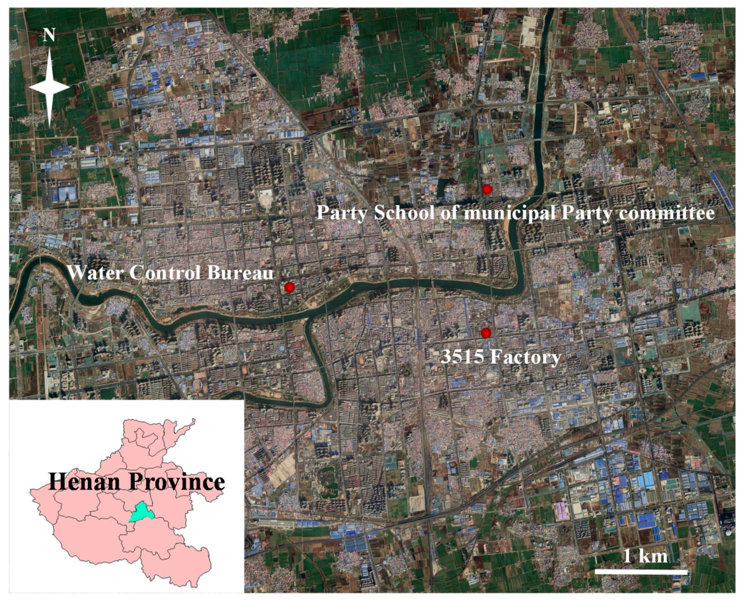
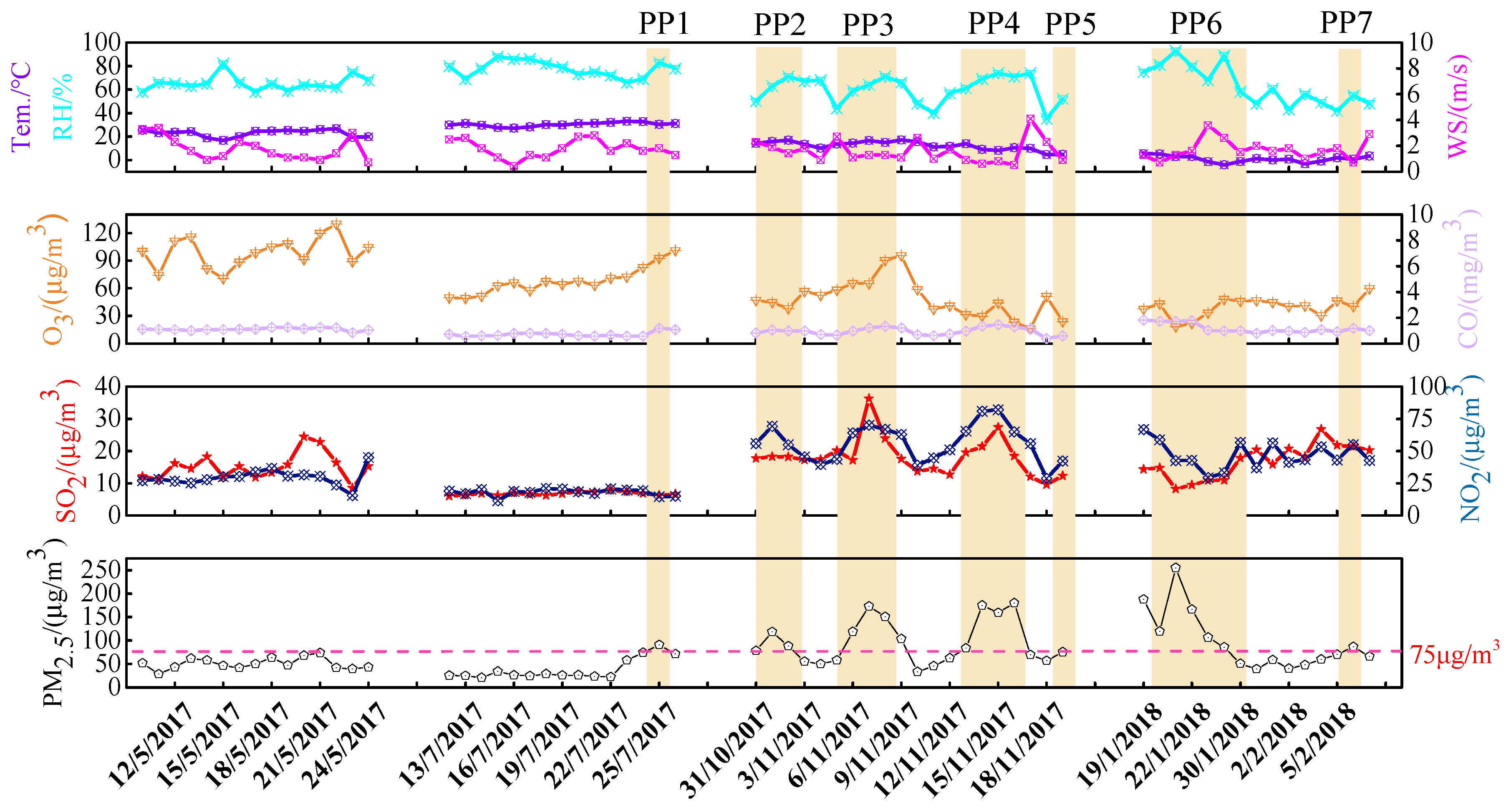
2.1. Sample Collection

This research is conducted in the urban area of Luohe City, which is located in the middle of Henan Province in China. The terrain is high in the northwest (~102 m above sea level) and low in the southeast (~50 m above sea level). It has a warm and humid monsoon climate. The total area is 2617 km² and the urban area is 72 km². The resident population is 2,650,000 and the urban resident population is 1,350,000 (Henan Statistical Yearbook, 2018, China Statistics Press [19]). The main industry in Luohe city is food processing—including meat processing, beverage production, instant noodle production, and so on. It is representative of a light industrial city, typically characterized by more consumer-oriented goods [20].

Three sampling sites were selected: the Luohe Water Control Bureau (114.03 E, 33.59 N), the Party School of the Municipal Party Committee (114.07 E, 33.60 N) and the 3515 factory (114.06 E, 33.57 N), which are shown in Figure 1. These sampling points are located in the centre of the city, no more than 5 km between any two sampling sites. The sampling times were as follows: (1) Spring: 10–24 May 2017; (2) Summer: 12–26 July 2017; (3) Autumn: 31 October–19 November 2017; (4) Winter: 19 January–7 February 2018. PM_2.5 membranes were collected from 11:00 a.m. to 10:00 a.m. the next day. The particulate membrane sampler (16.7 L/min) meets the European standard and the American standard (DERENDA PNS, Germany). Samples were collected simultaneously using a quartz filter and a Teflon filter, which are 47 mm in diameter. A total of 382 filters were collected. Among them, the quartz filters were used to analyse ions and carbon components, and the Teflon filters were used to analyze elemental components. The filter samples were weighed with a filter automatic weighing system (Commodore AWS-1, Germany) before and after sampling.

To understand the divergence of PM_2.5 and its chemical composition between different sampling sites, the coefficient of divergence (COD) was calculated.

$${\mathrm{COD}}_{\mathrm{jk}}=\sqrt{\frac{1}{\mathrm{P}}{\displaystyle \sum }_{\mathrm{i}=1}^{\mathrm{P}}(\frac{{\mathrm{x}}_{\mathrm{ij}}-{\mathrm{x}}_{\mathrm{ik}}}{{\mathrm{x}}_{\mathrm{ij}}+{\mathrm{x}}_{\mathrm{ik}}}}{)}^2$$

(1)

where COD_ij is the coefficient of divergence, j and k are the component spectrum numbers participating in the calculation, P is the number of chemical components participating in the calculation, and x_ij and x_ik represent the average concentration for a chemical component i at site j and k, respectively. It has been reported that if COD approaches 0, concentrations can be considered to be spatially homogeneous; if the COD was close to 1, the difference was more significant [21,22]. Results showed that the COD value ranged from 0.07 to 0.18 in this study. Therefore, the spatial variation of PM_2.5 and its chemical composition was not significant. The average value from three sites is thus used in subsequent discussions.

2.2. Chemical Composition Analysis

The organic carbon (OC) and elemental carbon (EC) were analysed by a thermal/optical carbon analyser (2001A, the American Desert Research Institute, USA) and the IMPROVE programmed temperature method was used [23].

Ion chromatography (ICS-2100, ICS-1100, Dionex, USA) was used to analyse four anions (F⁻, Cl⁻, NO₃⁻, SO₄²⁻) and five cations (Na⁺, K⁺, NH₄⁺, Ca²⁺, Mg²⁺) [24]. Cation concentrations were determined using a CS12-A (4 × 250 mm), with 20 mmol/L methane sulfonate as an eluent. The anions were separated using an AS11-HC (4 × 250 mm), with 1 to 30 mmol/L KOH as an eluent. The specific method is described in detail in previous research [25].

Elements (Li, Be, Na, P, K, Sc, As, Rb, Y, Mo, Cd, Sn, Sb, Cs, La, V, Cr, Mn, Co, Ni, Cu, Zn, Ce, Sm, W, Tl, Pb, Bi, Th, U) were analyzed by an inductively coupled plasma mass spectrometer (ICP-MS, Agilent 7500a, USA) while other elements (Zr, Al, Sr, Mg, Ti, Ca, Fe, Ba, Si) were analyzed by an inductively coupled plasma atomic emission spectrometer (ICP-OES, USA) [26].

For the elements, mineral dust (MD) was calculated using formula (2) [27,28].

$$\mathrm{MD}=1.89\mathsf{\rho }\left(\mathrm{Al}\right)+2.14\mathsf{\rho }\left(\mathrm{Si}\right)+1.4\mathsf{\rho }\left(\mathrm{Ca}\right)+1.43\mathsf{\rho }\left(\mathrm{Fe}\right)+1.67\mathsf{\rho }\left(\mathrm{Ti}\right)+1.2\mathsf{\rho }\left(\mathrm{K}\right)+1.66\mathsf{\rho }\left(\mathrm{Mg}\right)$$

(2)

where ρ(Al), ρ(Si), ρ(Ca), ρ (Fe), ρ(Ti), ρ(K), and ρ(Mg) are the concentrations of Al, Si, Ca, Fe, Ti, K, and Mg (μg/m³), respectively. TE is a simple addition of trace elements other than crustal elements and sea salt elements [29].

In order to analyze ions, the testing of a standard solution and a blank was performed before the targeted sample analysis, and the correlation coefficients of the standard samples were above 0.999. The method detection limits of F⁻, Cl⁻, NO₃⁻, SO₄²⁻, Na⁺, K⁺, NH₄⁺, Ca²⁺, and Mg²⁺ were 0.026, 0.058, 0.013, 0.010, 0.013, 0.087, 0.048, 0.084, and 0.067 mg L⁻¹, respectively. With regard to the analysis of the trace elements, the relative standard deviations between the real values of the standard materials and the analysis results were within a range of 2–15%, and the detection limits ranged from 0.00001 to 0.0005 μg L⁻¹. For carbonaceous species, 1 in every 10 samples was detected twice and the precision was less than 1%. Standard concentrations of CH₄/CO₂ mixed gases were used to calibrate the analyzer each day before and after the sample analysis. All the reported data for water-soluble ions, trace elements, and carbonaceous species were corrected by the filter blanks.

2.3. PMF Model

PMF (positive matrix factorization) is a multivariate receptor model, which is often used to study the PM source apportionment to obtain the type of pollution source and its contribution to PM [30,31,32].

In this work, Model PMF 5.0 (EPA, DurhamNC, USA) was used to conduct the receptor-based source apportionment for PM_2.5. The recommended approach in previous studies was used to come to a suitable solution [33]. The PMF model was run several times with the number of source factors ranging from three to seven. A higher number improved the fit marginally, but also resulted in factors that contributed little to the total PM_2.5 mass. Meanwhile, the possible sources impacting PM_2.5 mass concentration in the study area was considered [34,35].

2.4. Health Risk Estimation

According to the method described by the US Environmental Protection Agency (USEPA, 1989 [36]), several steps were used to develop the risk evaluation of metals in PM_2.5, including the calculation for the 95% upper confidence limit (UCL) of the arithmetic mean concentration, evaluating the exposure, and calculating the risk [31]. Nine heavy metals are considered in this study: Pb, Cr, Co, Ni, Zn, As, Cd, V, and Mn. Due to incomplete data on hand-feeding and skin contact, this study only considered the carcinogenic and non-carcinogenic risks of respiratory pathways.

The heavy metal exposure intake (D_inh) is calculated as in formula (3)

$${\mathrm{D}}_{\mathrm{inh}}=\frac{\mathrm{C}\times \mathrm{InhR}\times \mathrm{EF}\times \mathrm{ED}}{\mathrm{BW}\times \mathrm{AT}}$$

(3)

where D_inh is the heavy metal exposure intake through breath inhalation, mg kg⁻¹ day⁻¹. C is the heavy metal exposure concentration, generally taking the 95% confidence interval upper limit, mg/m³. InhR is the inhalation rate (m³/day). EF is the exposure frequency, day/year. ED is the exposure duration (year). BW is the body weight (kg). AT is the averaging time, AT = ED × 365 (days) for non-carcinogenic risk and AT = 70 × 365 (days) for cancer risk. The parameters involved in the exposure assessment are described in Table S1 [37,38,39,40].

The hazard quotient (HQ) represents the health risk value of non-carcinogenic metals. The hazard index (HI) is the sum of the risk quotients of metals through various pathways. If HI > 1, it indicates that a non-carcinogenic toxic risk exists. If HI ≤ 1, it indicates that the non-carcinogenic effect is inappreciable. The calculation formulas are as [11]

$$\mathrm{HQ}=\frac{{\mathrm{D}}_{\mathrm{inh}}}{{\mathrm{R}}_{\mathrm{fd}}}$$

(4)

$$\mathrm{HI}={\displaystyle \sum }{\mathrm{HQ}}_{\mathrm{i}}$$

(5)

where R_fd is the reference dose, mg kg⁻¹ day⁻¹ (Table S2) [41].

As a step towards calculating the carcinogenic risk, lifetime average daily dose (LADD) for heavy metal exposure are calculated (Equation (6)).

$$\mathrm{LADD}=\frac{\mathrm{C}\times \mathrm{EF}}{\mathrm{AT}}\times \left(\frac{{\mathrm{InhR}}_{\mathrm{child}}\times {\mathrm{ED}}_{\mathrm{child}}}{{\mathrm{BW}}_{\mathrm{child}}}+\frac{{\mathrm{InhR}}_{\mathrm{adult}}\times {\mathrm{ED}}_{\mathrm{adult}}}{{\mathrm{BW}}_{\mathrm{adult}}}\right)$$

(6)

To evaluate the health risk for carcinogenic metals, incremental lifetime cancer risk (ILCRi) value was used. If the ILCR is greater than 10⁻⁶, it is considered to be a carcinogenic risk [42]. The calculation formula is

$$\mathrm{ILCRi}=\mathrm{LADD}\times \mathrm{SFa}$$

(7)

$$\mathrm{ILCR}={\displaystyle \sum }\mathrm{ILCRi}$$

(8)

where SFa is the slope factor in mg kg⁻¹ day⁻¹ (Table S2).

3. Results and Discussion

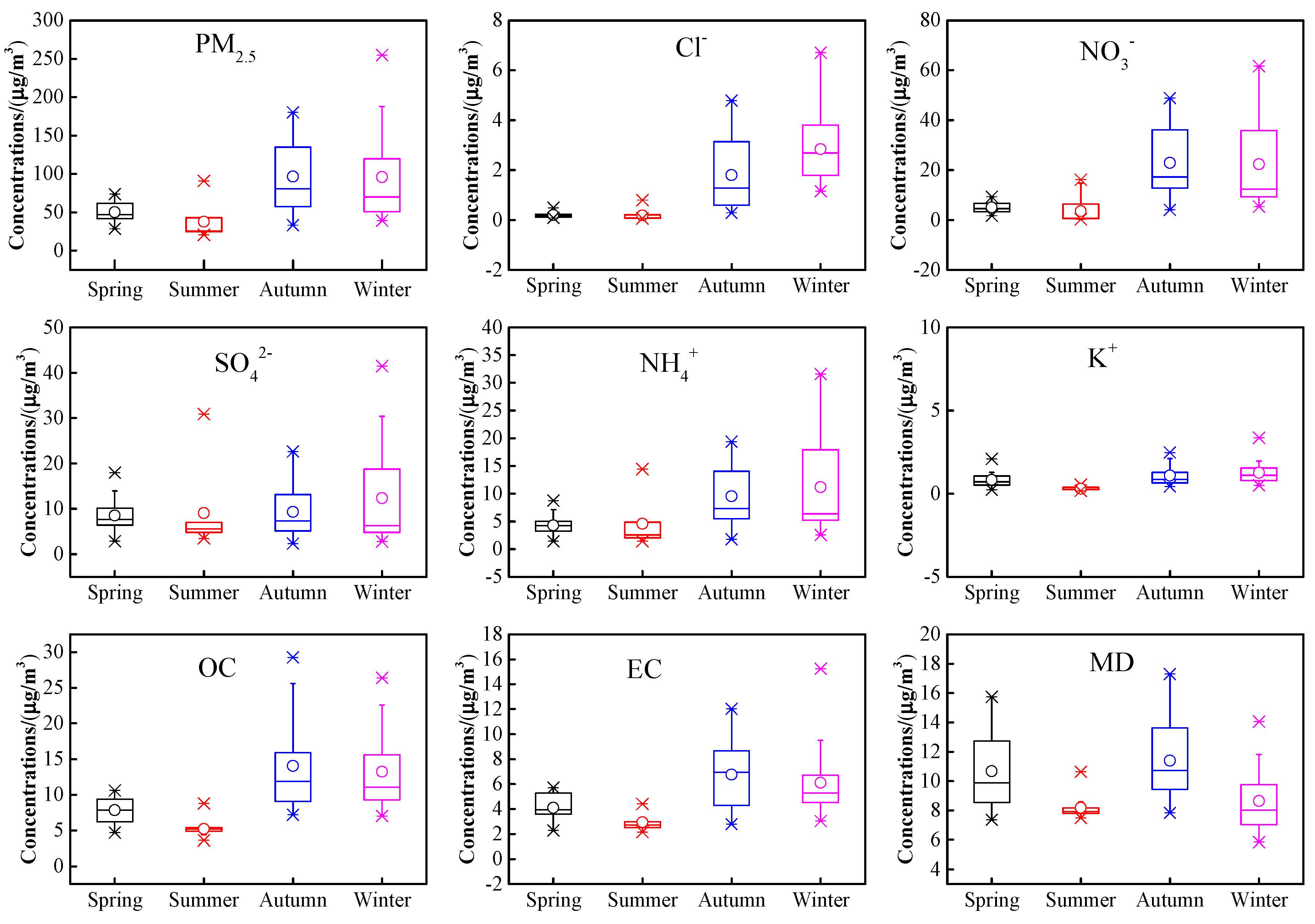
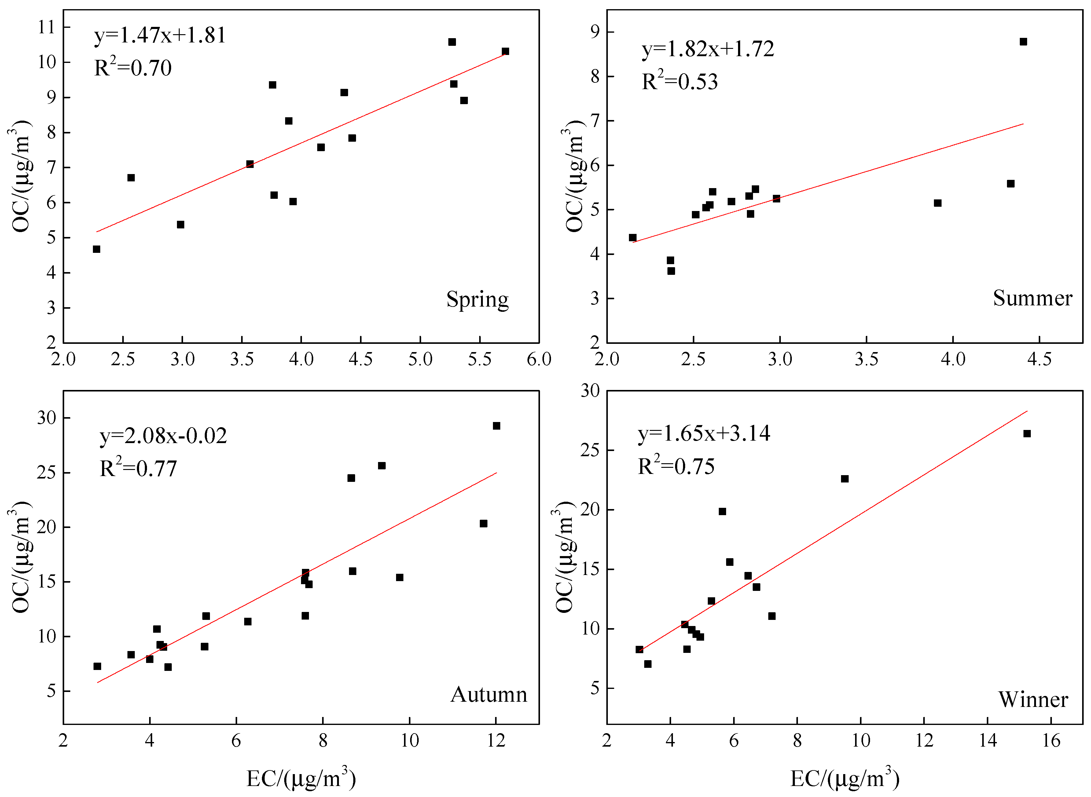
3.1. Chemical Composition

Figure 2 shows the variations of meteorological parameters, gaseous pollutants, and PM_2.5 during the campaign. There were several pollution episodes during the campaign. These pollution periods (PP) were defined as daily PM_2.5 concentrations being above 75 µg/m³. Meanwhile, the days with PM_2.5 concentrations below 75 µg/m³ were defined as clean periods (CP). Seven pollution episodes were identified during the campaign. There were three long-lasting pollution episodes that occurred between 6–9 November 2017; 13–16 November 2017; and 19–23 January 2018. The number of polluted days was 0, 1, 12, and 7 in the spring, summer, autumn, and winter, accounting for 0%, 6.7%, 60%, and 46.7% of the total sampling days in each season, respectively.

Table 1. Seasonal and annual average concentrations of PM_2.5 and of the major chemical species, as well as meteorological parameters and the concentrations of gaseous pollutants during the sampling period.

Species	Spring	Summer	Autumn	Winter	Annual
Meteorological parameters
Tem./(°C)	22.8 ± 3	30.3 ± 1.7	12.2 ± 3.6	−0.1 ± 2.2	16.2 ± 11.1
RH/%	65.3 ± 6.1	77.6 ± 6.6	60.2 ± 11.4	58.1 ± 13.9	66.0 ± 12.8
WS/(m/s)	1.8 ± 0.9	1.8 ± 0.7	1.6 ± 0.9	1.9 ± 0.8	1.7 ± 0.8
Concentrations of gaseous pollutants (µg/m3)
O3	99 ± 16	68 ± 14	48 ± 20	42 ± 9	63 ± 27
SO2	15 ± 4	7 ± 1	18 ± 6	18 ± 5	15 ± 6
NO2	30 ± 6	18 ± 3	56 ± 14	44 ± 9	39 ± 18
Concentrations of PM2.5 and chemical compositions (µg/m3)
PM2.5	51 ± 13	38 ± 22	97 ± 47	96 ± 61	73 ± 49
SO42−	8.6 ± 3.7	9 ± 7.8	9.3 ± 5.7	12.3 ± 11.2	9.8 ± 7.7
NO3−	5.2 ± 2.4	3.6 ± 5.3	22.9 ± 14.1	22.4 ± 17	14.4 ± 14.9
NH4+	4.4 ± 1.9	4.6 ± 4.3	9.5 ± 5.3	11.2 ± 8.5	7.7 ± 6.3
Cl−	0.2 ± 0.1	0.2 ± 0.2	1.8 ± 1.6	2.8 ± 1.5	1.3 ± 1.6
K+	0.9 ± 0.5	0.3 ± 0.1	1.1 ± 0.6	1.3 ± 0.7	0.9 ± 0.6
OC	7.9 ± 2.0	5.2 ± 1.2	14 ± 6.6	13.2 ± 5.5	10.4 ± 6
EC	4.1 ± 1.2	2.9 ± 0.7	6.8 ± 2.8	6.1 ± 3	5.1 ± 2.7
MD	10.7 ± 2.4	8.1 ± 0.8	11.3 ± 2.7	8.6 ± 2.2	9.8 ± 2.6
TE	0.5 ± 0.1	0.3 ± 0.1	0.6 ± 0.2	0.7 ± 0.2	0.6 ± 0.2

Note: WS—wind speed; Tem.—temperature; RH—relative humidity; MD—mineral dust, TE—trace elements.

presents seasonal and annual mean concentrations of PM_2.5 and its major chemical components during the sampling periods. During the sampling period, the mean temperature was 16.2 ± 11.1 °C and the RH was 66.0 ± 12.8% on average. The average wind speed was 1.7 ± 0.8 m/s over the whole sampling period. Daily PM_2.5 ranged from 21 to 255 µg/m³, with an annual average of 73 ± 49 µg/m³. The average concentrations of PM_2.5 in autumn (97 μg/m³) and winter (96 μg/m³) were much higher than that in spring (51 μg/m³) and summer (38 μg/m³).

The contribution of different compositions to PM_2.5 varied widely (Figure S1). For water soluble ions, SO₄²⁻, NO³⁻, and NH₄⁺ were the main ions, accounting for 13%, 20%, and 11% of PM_2.5 mass in terms of an annual average, respectively. The sum of SO₄²⁻, NO₃⁻, and NH₄⁺ (SNA) was 31.9 µg/m³, contributing 44% to PM_2.5 mass. For carbonaceous components, organic matter (OM) was the most abundant species in PM_2.5. OM was estimated from OC using a conversion factor of 1.4 to account for other elements presented in organic compounds [43], and accounted for 20% of PM_2.5 mass. Meanwhile, the EC proportion was relatively low and only accounted for around 7%. MD was 9.8 µg/m³ and accounted for 13% of PM_2.5 mass. The other portions of PM_2.5 reached 17%, which were likely related to the uncertainties in the multiplication factors used for estimating OM and MD, other unidentified species, and measurement uncertainties. In total, the sum of the secondary inorganic ions and carbonaceous species accounted for 64% of PM_2.5 mass and were the main component.

Table 1 also shows the seasonal average concentrations of PM_2.5 and its major chemical components during the sampling periods. Meanwhile, Figure 3 shows the seasonal distributions of PM_2.5 and its major chemical components. PM_2.5 mass in winter and autumn was 0.9–1.6 time higher (interquartile ranges) than those in the other seasons, and there was not much difference in these two seasons. The chemical components basically follow the seasonal variation of the PM_2.5 mass concentration. In terms of MD, its concentration was highest in autumn, followed by spring, winter, and summer. Regarding SO₄²⁻, its average concentration was highest in winter and the difference in the other three seasons was not significant. The average temperature in the winter was −0.1 ± 2.2 °C. Though no central heating exists in the urban area, residential coal combustion for heating is absolutely necessary. Therefore, residential coal combustion might be the main reason for the high sulphate concentrations in winter.

It should also be noted that the seasonal variation of NO₃⁻ was much larger than those of SO₄²⁻ and NH₄⁺. The average concentration of NO₃⁻ in autumn and winter was 4.1 times higher than in the spring and the summer. Atmospheric physicochemical processes played an important role [44]. The concentration of NO₃⁻ might have been enhanced in the winter under high RH through heterogeneous aqueous processes and decreased in the summer due to the volatilization of NH₄NO₃ under high temperatures.

To investigate the source of carbon compositions, the correlation between OC and EC was analyzed (Figure 4). As reported in the literature, OC was mainly derived from fossil fuel combustion, biomass burning and secondary organic aerosols generated by atmospheric chemical reactions, which were susceptible to weather conditions and emission sources [30,45]. EC was mainly derived from fossil fuel combustion and it was an inert pollutant. If the correlation coefficient between OC and EC was greater than 0.65, the source of OC and EC was considered to be consistent [46]; otherwise, the source of the two was complicated. In this study, there was good correlation for OC and EC in spring, autumn, and winter, indicating the same pollution sources. Regarding summer, the relatively low correlation between OC and EC indicated the different sources of OC and EC in the summer, which was related to the fact that OC was partly derived from secondary aerosol generation in the summer.

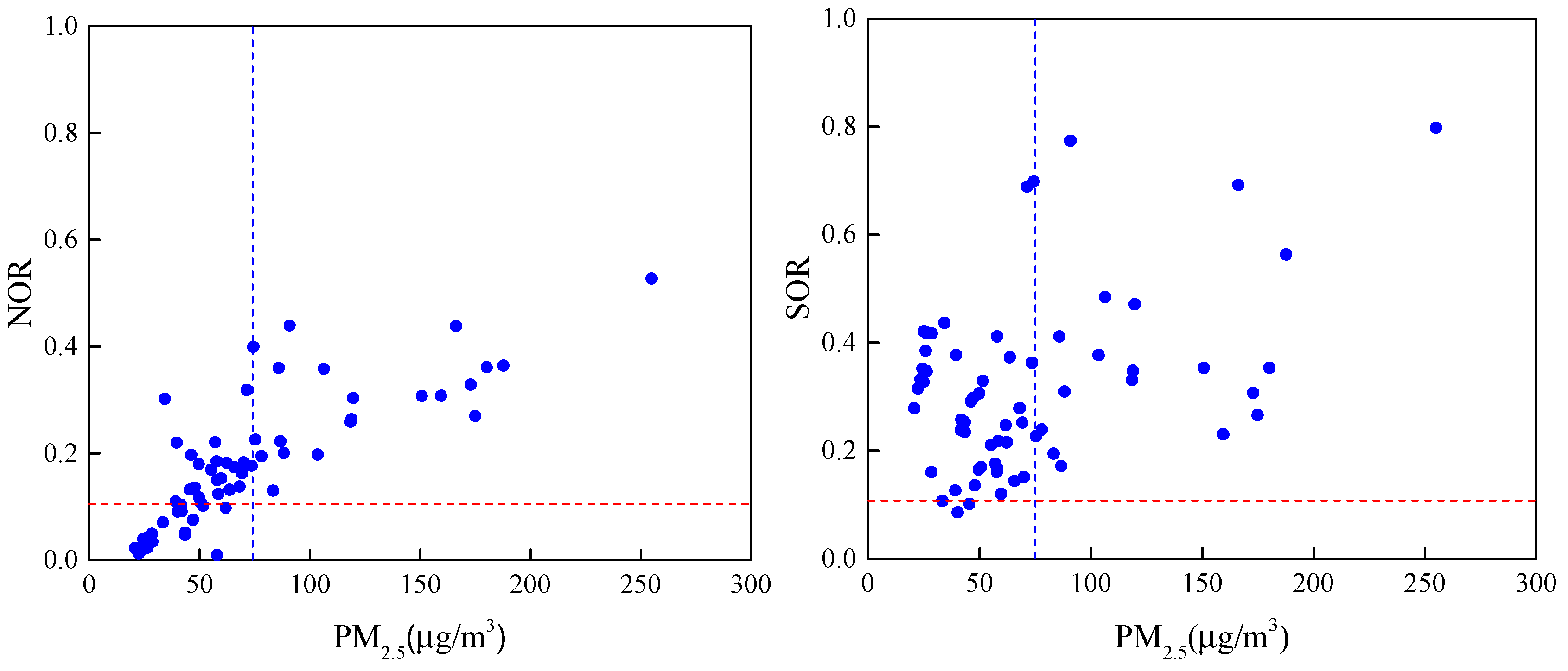
3.2. Comparison of Chemical Composition on Clean and Polluted Days

The concentrations of PM_2.5 and major chemical components increased dramatically on polluted days compared with clean days (

Table 2. Average concentration of major chemical components in PM_2.5 on clean days and polluted days.

Period	Concentration	PM2.5	SO42−	NO3−	NH4+	Cl	K	OM	EC	MD	Other
Clean day	Mass concentration (μg/m3)	46	7.0	5.5	4.2	0.8	0.6	10.5	4.0	10.2	3.2
	Proportion (%)	/	15	12	9	2	1	23	9	22	7
Polluted day	Mass concentration (μg/m3)	130	16.5	31.4	14.7	2.5	1.5	23.7	8.3	12.1	19.3
	Proportion (%)	/	13	24	11	2	1	18	6	9	15

Note: MD—mineral dust.

). The average concentrations of PM_2.5 on polluted days (130 μg/m³) were 1.8 times higher than on clean days (46 μg/m³), and the concentrations of the two dominant groups of components, SNA and OM, were 2.7 and 2.3 times higher than on clean days. The contribution of SNA to PM_2.5 on polluted days was 48%, which was higher than that on clean days (36%). Compared with clean days, concentrations of the individual SNA species (SO₄²⁻, NO₃⁻, and NH₄⁺) increased by a factor of 1.4–4.7 on polluted days. However, the proportion of each chemical composition differed across different days with increasing NO₃⁻ and decreasing SO₄²⁻ on polluted days. The proportion of OM in PM_2.5 decreased from 23% on clean days to 18% on polluted days.

Stagnant atmospheric conditions and high RH were important factors causing PM_2.5 pollution events [47,48,49]. Weak winds suppressed pollutant dispersion vertically and horizontally [50]. High RH was also conducive for aqueous-phase reactions and resulted in the rapid elevation of SO₄²⁻ and NO₃⁻ concentrations [51,52,53]. Compared with the clean periods in the same season, the pollution periods were usually characterized by high temperatures and weak wind speeds in this study. For RH, the seasonal variation was small, ranging from 58.1% (in winter) to 77.6% (in summer) with an annual average of 66.0%. This high humidity was favorable for aqueous-phase reactions.

In order to characterise the conversion degree of gaseous SO₂ and NO₂ to SO₄²⁻ and NO₃⁻ ions, SOR (sulfur oxidation rate) and NOR (nitrogen oxidation rate) are usually used [54]. Studies have shown that when the values of SOR and NOR were < 0.1, the pollutants mainly stemmed from direct discharge, and when the value was > 0.1, it means that there was a secondary conversion of primary pollutants [55,56]. In this study, the values of NOR and SOR in different PM_2.5 concentrations are shown in Figure 5. The average values of NOR were 0.30 (on polluted days) and 0.12 (on clean days), respectively. The average values of SOR were 0.40 (on polluted days) and 0.28 (on clean days), respectively. All the SOR and NOR values were greater than 0.1 on polluted days, and the increase in NOR on polluted days was greater than SOR. This explained the large variation of NO₃⁻ in the four seasons and the high proportion of NO₃⁻ on polluted days.

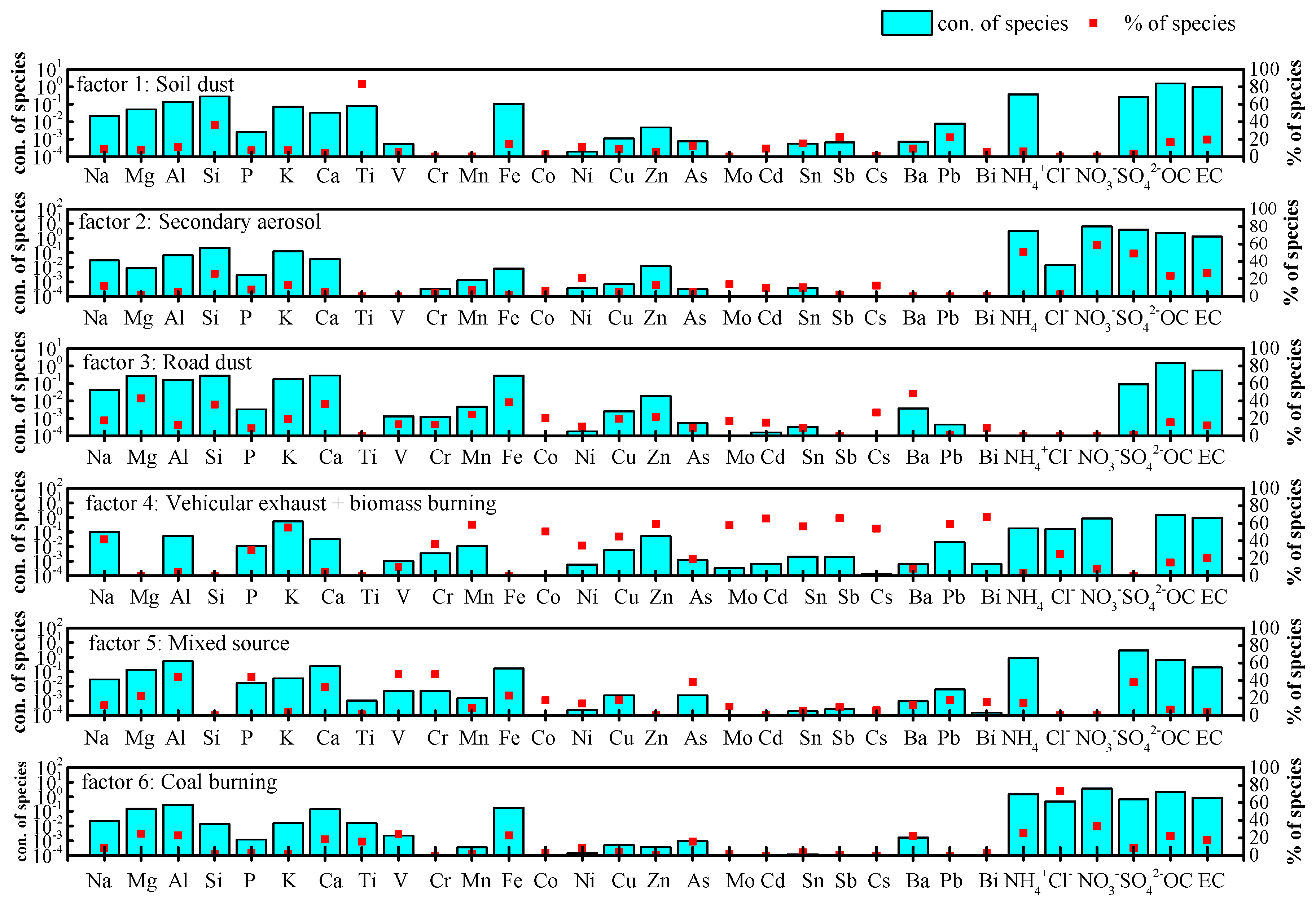
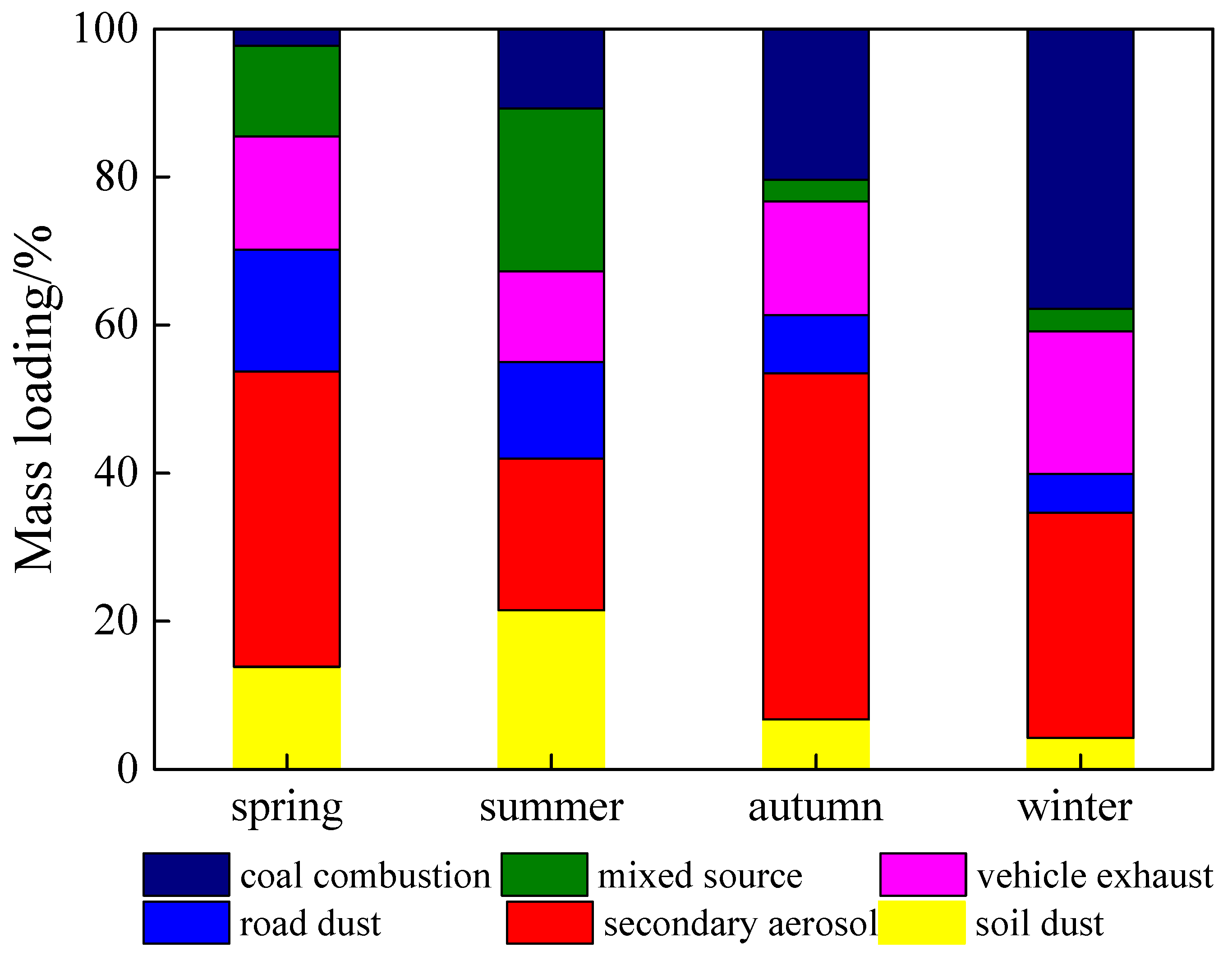
3.3. Sources Apportionment of PM_2.5

The positive matrix factorization (PMF, version 5.0) was applied to elucidate the source–receptor relationship of PM_2.5. We examined a wide range of factor solutions (4–7). The recommended approach in previous studies was used to come to a suitable solution [33]. Six factors were identified by PMF analysis, and the factor profiles are shown in Figure 6. The correlation coefficient R² between the fitted value and the measured value of PM_2.5 was 0.68, indicating that the analytical result was reasonable.

In factor 1, Ti (83%) and Si (36%) accounted for high proportions. These elements were mainly crust elements [57], so this factor was judged to be a soil dust source. Factor 2 was remarkably characterized by NO₃⁻ (59%), SO₄²⁻ (49%), and NH₄⁺ (51%), and was determined to be a secondary source. In factor 3, Mg (43%), Ca (36%), Si (36%), Fe (39%), and Zn (22%) accounted for high proportions. Mg, Ca, and Si were mainly crust elements [58]. Fe and Zn may come from tire wear and metal parts wear [41,59,60]. Therefore, this factor was judged to be a dust source. Factor 4 contains a high proportion of Zn (59%), Sn (56%), Pb (59%), Cu (45%), and K (55%). The metallic elements were usually derived from traffic pollution sources such as fuel combustion, tire wear, oil leakage, and wear of batteries and metal parts [41,59,60,61]. K is often used as a tracer of biomass burning. Considering the biomass burning in the suburban area, this factor is determined to be a mixed source of vehicle exhaust and biomass burning. Factor 5 displays high loadings for Cr (47%), with median loads of Fe (23%), Cu (18%), Pb (18%), Ni (14%), and NH₄⁺ (14%). Cr is a tracer of dust. As well as soil dust and road dust, construction dust is an important source of dust. The presence of many metals could be attributed to metal industry activities [62,63]. Aside from secondary aerosols, NH₄⁺ is related to the source emissions from agriculture, livestock, and poultry. Because of the food processing industry in this city, there were several atmospheric pollutant emission sources such as animal feeding, the use of spices, packaging material production, fossil fuel combustion, and so on. Therefore, this factor was determined to be a mixed source (construction dust, metal industry, livestock and poultry breeding, food processing industry, and so on). Factor 6 displays a high proportion of Cl⁻ (73%), NO₃⁻ (33%), V (24%), and OC (22%). Cl⁻ is a tracer of coal combustion in inland areas [64]. NO₃⁻ is mainly converted from NOx, which was emitted from fossil fuel combustion. The V element also acted as a typical tracer of fossil fuel combustion [65]. Therefore, this factor is determined to be coal combustion.

Seasonal contributions of each source are shown in Figure 7. Secondary sources are the largest part in each season. The secondary sulfate, nitrate, and ammonia salt are likely to be associated with the formation of primary pollutants emitted from coal combustion, vehicle exhaust, livestock and poultry breeding, and so on. Emissions from livestock and poultry were the most important source in the summer and the spring when the temperature was high. In the autumn and the winter, the appearance of adverse meteorological conditions usually occurred, which led to atmospheric pollution as well as the formation and accumulation of secondary pollutants. In line with the volatilization of NH₄NO₃ under high temperatures in the summer, the contribution of secondary sources was low in the summer.

Luohe city is located in Henan province, which is an agriculture province. Therefore, in the spring and the summer, the contribution of soil dust is relatively high because of agricultural activity. Road dust and vehicle exhaust sources are steady across the four seasons. Because of the need for heating in late autumn and the winter, coal combustion and biomass burning played an important role. Vehicle exhaust and biomass sources increased slightly and coal combustion sources increased significantly in the autumn and the winter. Except metal industry, the other parts in the mixed source (construction dust, metal industry, livestock and poultry breeding, food processing industry, and so on) are active in the spring and the summer. Therefore, the mixed sources in the spring and the summer were much higher than in the autumn and the winter.

The source percentage contributions of each source to PM_2.5 are shown in

Table 3. Comparison of source apportionment with other cities.

City	Method		Source Contribution (%)							Reference
	Sampling	Model	Coal Combustion	Industrial Emission	Secondary Aerosol	Dust	Vehicle Exhaust	Biomass Burning	Other Sources
Luohe, China	2017–2018, Urban, clean days	PMF	11		28	Soil dust: 12 Road dust: 13	16		Mixed source (husbandry and food procession industry): 21	This study
	2017–2018, Urban, pollution days	PMF	2		49	Soil dust: 6 Road dust: 5	17		Mixed source (husbandry and food procession industry): 21	This study
Zhengzhou China	2013–2015 Pollution days	CMB	14	8	Nitrate: 13 Sulfate: 16	8	7	12	carbon + refractory material: 2	[66]
	2013–2015 Other days	CMB	27	9	Nitrate: 20 Sulfate: 18	14	15	9	carbon + refractory material: 2
Xiangtan China	2016–2017 urban	PMF		6–9	Secondary inorganic aerosols: 25–27	16–18	21–22		coal combustion + secondary aerosols: 19–21 steel industry: 8–9	[69]
Lanzhou China	2012 winter urban	PMF	28.7		33.0	13.3	8.8		Steel industry: 7.1 Power plant: 3.12 Smelting industry: 6.0	[67]
	2013 summer urban	PMF	3.1		14.8	11.6	25.2		Steel industry: 6.7 Power plant: 3.4 Smelting industry: 35.2
Xian China	1.1.–2.28. 2006. urban	PMF	31.2	9.8	20.9	12.8	19.3	6.0		[68]
	1.1.–2.28. 2008. urban	PMF	27.6	11.5	23.2	11.7	20.9	5.1
	1.1.–2.28. 2010. urban	PMF	24.1	12.6	17.5	19.4	21.3	5.1
Taian China	8–9.11. 2014. urban	PMF	17.94	9.41	27.47		16.65		Metal manufacturing: 19.06 other: 9.47	[70]
New York, USA	June–July 2009, 2010, urban	PMF			sulfate:35 nitrate:14	14	16		Aged sea-salt: 9 residual oil: <5 fresh sea-salt: <5	[34]
Dongguan China	2014 Suburb	PMF	5–8	5–8	Nitrate:5–8 Sulfate:20 secondary organic:10	5–8	21	11	Ship emission: 5–8	[71]
Fort McKay, Canada	March 2009–January 2011 suburb	PMF			Secondary sulfate: 30.77		Fugitive dust: 32.4		Secondary nitrate/biomass burning: 26.4 Mining/mobile: 10.1 Other: 0.4	[6]

Note: PMF—positive matrix factorization. CMB—chemical mass balance.

. For comparison, source apportionment results on polluted and clean days as well as other cities are also listed in Table 3. The most important source of PM_2.5 was secondary aerosols both on clean days (28%) and polluted days (49%). Coal combustion made a relatively low contribution to PM_2.5, which was in line with the light industry characteristics. Soil dust and road dust contributed 11–25% to PM_2.5, which was similar to many cities such as Zhengzhou [66], Lanzhou [67], and Xian [68] in China, as well as New York in USA [34]. The contribution proportion of secondary aerosol sources to PM_2.5 on polluted days was 1.75 times that of clean days, while coal combustion and dust (soil dust and road dust) sources contributed a lower proportion to PM_2.5 on polluted days than on clean days. Certain identified sources, such as coal combustion and vehicle exhaust, could also promote the production of secondary inorganic and organic aerosols through the precursor gases [17]. These source apportionment results confirmed the importance of the chemical reaction process to secondary aerosol formation.

3.4. Health Risk Evaluation of Heavy Metals

Some health effects of atmospheric particulate matter can be recognized by assessing the exposure of heavy metals to human bodies. Because of individual differences, these estimations are preliminary estimations and can only be regarded for screening purposes [72].

The daily exposure concentration and health risk value of heavy metals in PM_2.5 are shown in

Table 4. Annual heavy metal inhalation exposure concentrations and health risks.

Element	Child Intake Dinh(Child) mg kg−1 day−1	Adult Intake Dinh(Adult) mg kg−1 day−1	Lifetime Intake LADD mg kg−1 day−1	Child Risk Index HI	Adult Risk Index HI	Carcinogenic Risk mg kg−1 day−1
V	7.31 × 10−7	3.65 × 10−7		1.04 × 10−4	5.21 × 10−5
Cr	2.11 × 10−6	1.05 × 10−6	7.42 × 10−6	7.38 × 10−2	3.68 × 10−2	3.11 × 10−4
Mn	3.65 × 10−6	1.82 × 10−6		2.61 × 10−1	1.30 × 10−1
Co	4.12 × 10−8	2.05 × 10−8	1.45 × 10−7	7.21 × 10−3	3.60 × 10−3	1.42 × 10−6
Ni	3.82 × 10−7	1.91 × 10−7	1.34 × 10−6	1.86 × 10−5	9.26 × 10−6	1.13 × 10−6
Zn	2.61 × 10−5	1.30 × 10−5		8.66 × 10−5	4.32 × 10−5
As	4.98 × 10−7	2.48 × 10−7	1.75 × 10−6	1.65 × 10−3	8.25 × 10−4	2.64 × 10−5
Cd	4.46 × 10−7	2.23 × 10−7	1.57 × 10−6	4.46 × 10−4	2.23 × 10−4	1.00 × 10−5
Pb	7.68 × 10−6	3.83 × 10−6		2.18 × 10−3	1.09 × 10−3
∑	4.16 × 10−5	2.08 × 10−5	1.22 × 10−5	3.46 × 10−1	1.73 × 10−1	3.50 × 10−4

. For a non-carcinogenic risk assessment, the risk index (HI) of non-carcinogenic heavy metals through the respiratory route were 1.86 × 10⁻⁵~0.261 and 9.26 × 10⁻⁶~0.130 for children and adults, respectively. Since the risk index (HI) does not exceed 1, non-carcinogenic hazard is not expected to occur for people. In terms of carcinogenic hazard, Cr, Co, Ni, As, and Cd exceeded the risk threshold of 10⁻⁶ and had carcinogenic hazard. Among them, the carcinogenic risk of Cr was at its highest at 3.11 × 10⁻⁴. Therefore, we should pay special attention to these heavy metals in PM_2.5 with high carcinogenic risks for residents.

As shown in

Table 5. Annual mass, risk index HI, and carcinogenic risk Rt of six identified sources of PM_2.5.

Sources	Soil Dust	Secondary Aerosol	Road Dust	Vehicle Exhaust	Mixed Source	Coal Combustion
Mass concentration (μg/m3)	5.75	23.33	5.81	10.03	4.42	12.97
HI Child	9.25 × 10−4	2.08 × 10−2	7.54 × 10−2	1.85 × 10−1	5.86 × 10−2	5.35 × 10−3
HI Adult	4.62 × 10−4	1.04 × 10−2	3.76 × 10−2	9.23 × 10−2	2.92 × 10−2	2.67 × 10−3
Rt	4.29 × 10−6	1.35 × 10−5	4.50 × 10−5	1.26 × 10−4	1.58 × 10−4	4.35 × 10−6

, vehicle exhaust sources are the largest HI contributor, accounting for 54%. Vehicle exhaust and mixed sources are the main Rt contributor, accounting for 36% and 45%, respectively. Similar findings have been reported by previous studies [72,73]. The contribution of sources to PM_2.5 mass concentration was also listed in Table 5. It is obvious that the source contribution for mass and health risks are different. Secondary sulfate contributed the most (37%) to PM_2.5 mass and only accounted for 6% of HI and 4% of Rt. However, vehicle sources contributed 16% to PM_2.5 mass and accounted for 54% of HI and 36% of Rt. Therefore, PM control strategies should highlight sources with more toxic components such as trace heavy metals.

4. Conclusions

To study the chemical composition and health risk of PM_2.5 in a city with light industry as its main industry, a total of 382 PM_2.5 filter samples were collected in four seasons (15–20 days for each season) from May 2017 to February 2018 in the urban area of Luohe city. PM_2.5 concentrations and chemical compositions were analyzed. Representative elemental components (V, Cr, Mn, Co, Ni, Zn, As, Cd, P) of PM_2.5 were applied to assess health risk.

During the sampling period, the annual PM_2.5 value was 73 ± 49 μg/m³. Seasonal variations of PM_2.5 concentrations and major chemical components were significant, usually with high mass concentrations in the autumn (97 μg/m³) and the winter (96 μg/m³), and with low mass concentrations in the spring (51 μg/m³) and the summer (38 μg/m³). SNA (SO₄²⁻, NO₃⁻, and NH₄⁺) was the most abundant component, and the sum of the SNA was 31.9 µg/m³, contributing 43.8% to PM_2.5 mass. PM_2.5 concentrations were more than two times higher on polluted days than on clean days, and the two dominant groups of components (SNA and OC) were 2.3–3.7 times higher than on clean days. The values of SOR were 0.40 (on polluted days) and 0.28 (on clean days), respectively. The most important source of PM_2.5 was secondary aerosols, both on clean days (28%) and polluted days (49%). A stagnant atmosphere and high relative humidity were the meteorological conditions for the formation of pollution. Secondary aerosol generation was one main reason for the variation of chemical composition proportions on different polluted days.

The health risk assessment of heavy metals showed that non-carcinogenic risk was not appreciable, while the carcinogenic risk exceeded the risk threshold of 10⁻⁶. Vehicle exhaust and mixed sources (construction dust, metal industry, livestock and poultry breeding, and food processing industries) are the main Rt contributor, accounting for 36% and 45%, respectively. Therefore, we should pay special attention to the heavy metal elements in PM_2.5. In the future, more research needs to be conducted in order to master the pollution characteristics of such cities and to provide scientific support for the government to make policies for atmospheric pollution prevention and control.

References

1. Shuang, Y.Y.; Liu, W.J.; Xu, Y.S.; Yi, K.; Zhou, M.; Tao, S.; Liu, W.X. Characteristics and oxidative potential of atmospheric PM2.5 in Beijing: Source apportionment and seasonal variation. Sci. Total Environ. 2019, 650, 277–287. [Google Scholar]
2. Lee, C.G.; Yuan, C.S.; Chang, J.C.; Yuan, C. Effects of aerosol species on atmospheric visibility in Kaohsiung City, Taiwan. Air Waste Manag. 2005, 55, 1031–1041. [Google Scholar] [CrossRef] [Green Version]
3. Cui, G.; Zhang, Z.; Lau, A.K.H.; Chang, Q.L.; Lao, X.Q. Effect of long-term exposure to fine particulate matter on lung function decline and risk of chronic obstructive pulmonary disease in Taiwan: A longitudinal, cohort study. Lancet Planet. Health 2018, 2, 114–125. [Google Scholar]
4. Ai, S.; Qian, Z.M.; Guo, Y.; Yang, Y.; Rolling, C.A.; Liu, E.; Wu, F.; Lin, H. Long-term exposure to ambient fine particles associated with asthma: A cross-sectional study among older adults in six low- and middle-income countries. Environ. Res. 2019, 68, 141–145. [Google Scholar] [CrossRef]
5. Agarwal, A.; Mangal, A.; Satsangi, A.; Lakhani, A.; Kumari, K.M. Characterization, sources and health risk analysis of PM2.5 bound metals during foggy and non-foggy days in sub-urban atmosphere of Agra. Atmos. Res. 2017, 197, 121–131. [Google Scholar] [CrossRef]
6. Bari, M.A.; Kindzierski, W.B. Ambient fine particulate matter (PM2.5) in Canadian oil sands communities: Levels, sources and potential human health risk. Sci. Total Environ. 2017, 595, 828–838. [Google Scholar] [CrossRef] [Green Version]
7. Wang, Y.; Jia, C.; Tao, J.; Zhang, L.; Liang, X.; Ma, J.; Gao, H.; Huang, T.; Zhang, K. Chemical characterization and source apportionment of PM 2.5 in a semi-arid and petrochemical-industrialized city, Northwest China. Sci. Total Environ. 2016, 573, 1031–1040. [Google Scholar] [CrossRef]
8. Frederic, L.; Adib, K.; Gilles, D.; Gilles, R.; Atallah, E.Z.; Dominique, C. Contributions of local and regional anthropogenic sources of metals in PM2.5 at an urban site in northern France. Chemosphere 2017, 181, 713–724. [Google Scholar]
9. Wang, J.; Zimei, H.U.; Chen, Y.; Chen, Z.; Shiyuan, X.U. Contamination characteristics and possible sources of PM10 and PM2.5 in different functional areas of Shanghai, China. Atmos. Environ. 2013, 68, 221–229. [Google Scholar] [CrossRef]
10. Zheng, H.; Kong, S.; Yan, Q.; Wu, F.; Cheng, Y.; Zheng, S.; Wu, J.; Yang, G.; Zheng, M.; Tang, L.; et al. The impacts of pollution control measures on PM2.5 reduction: Insights of chemical composition, source variation and health risk. Atmos. Environ. 2019, 197, 103–117. [Google Scholar] [CrossRef]
11. Zhang, J.; Zhou, X.; Wang, Z.; Yang, L.; Wang, J.; Wang, W. Trace elements in PM2.5 in Shandong Province: Source identification and health risk assessment. Sci. Total Environ. 2018, 621, 558–577. [Google Scholar] [CrossRef] [PubMed]
12. Burnett, R.T.; Pope, C.A., III; Ezzati, M.; Olives, C.; Lim, S.S.; Mehta, S.; Shin, H.H.; Singh, G.; Hubbell, B.; Brauer, M.; et al. An integrated risk function for estimating the global burden of disease attributable to ambient fine particulate matter exposure. Environ. Health Perspect. 2014, 122, 397–403. [Google Scholar] [CrossRef] [PubMed]
13. Davidson, C.I.; Phalen, R.F.; Solomon, P.A. Airborne particulate matter and human health: A review. Aerosol Sci. Technol. 2005, 39, 737–749. [Google Scholar] [CrossRef]
14. Roksana, K.; Shoko, K.; Sheng, N.C.F.; Masahiro, U.; Ferdosi, K.A.; Saira, T.; Chiho, W. Association between short-term exposure to fine particulate matter and daily emergency room visits at a cardiovascular hospital in Dhaka, Bangladesh. Sci. Total Environ. 2019, 646, 1030–1036. [Google Scholar]
15. Yu, Y.; Yao, S.; Dong, H.; Wang, L.; Wang, C.; Ji, X.; Ji, M.; Yao, X.; Zhang, Z. Association between short-term exposure to particulate matter air pollution and cause-specific mortality in Changzhou, China. Environ. Res. 2019, 170, 7–15. [Google Scholar] [CrossRef] [PubMed]
16. Andersson, A.; Deng, J.; Du, K.; Zheng, M.; Yan, C.; Sköld, M.; Gustafsson, Ö. Regionally-varying combustion sources of the January 2013 severe haze events over eastern China. Environ. Sci. Technol. 2015, 49, 2038–2043. [Google Scholar] [CrossRef] [PubMed]
17. Zhang, J.K.; Sun, Y.; Liu, Z.R.; Ji, D.S.; Hu, B.; Liu, Q.; Wang, Y.S. Characterization of submicron aerosols during a month of serious pollution in Beijing, 2013. Atmos. Chem. Physics. 2014, 14, 1431–1432. [Google Scholar] [CrossRef] [Green Version]
18. Zheng, S.; Pozzer, A.; Cao, C.X.; Lelieveld, J. Long-term (2001–2012) fine particulate matter (PM2.5) and the impact on human health in Beijing, China. Atmos. Chem. Phys. 2015, 14, 5715–5725. [Google Scholar] [CrossRef] [Green Version]
19. Henan Province Bureau of Statistics; Henan Investigation Corps of National Bureau of Statistics. Henan Statistical Yearbook; China Statistics Press: Beijing, China, 2018.
20. Li, J.; Lin, B. Ecological total-factor energy efficiency of China’s heavy and light industries: Which performs better? Renew. Sustain. Energy Rev. 2017, 72, 83–94. [Google Scholar] [CrossRef]
21. Wilson, J.G.; Kingham, S.; Pearce, J.; Sturman, A.P. A review of intraurban variations in particulate air pollution: Implications for epidemiological research. Atmos. Environ. 2005, 39, 6444–6462. [Google Scholar] [CrossRef]
22. Bell, M.L.; Ebisu, K.; Peng, R.D. Community-level spatial heterogeneity of chemical constituent levels of fine particulates and implications for epidemiological research. J. Expo. Sci. Environ. Epidemiol. 2011, 21, 372–384. [Google Scholar] [CrossRef] [PubMed] [Green Version]
23. Chow, J.C.; Watson, J.G.; Lu, Z.; Lowenthal, D.H.; Frazier, C.A.; Solomon, P.A.; Thuillier, R.H.; Magliano, K. Descriptive analysis of PM2.5 and PM10 at regionally representative locations during SJVAQS/AUSPEX. Atmos. Environ. 1996, 30, 2079–2112. [Google Scholar] [CrossRef]
24. Meng, C.C.; Wang, L.T.; Zhang, F.F.; Wei, Z.; Ma, S.M.; Ma, X.; Yang, J. Characteristics of concentrations and water-soluble inorganic ions in PM2.5 in Handan City, Hebei province, China. Atmos. Res. 2016, 171, 133–146. [Google Scholar] [CrossRef]
25. Wang, N.; Yin, B.H.; Wang, J.; Liu, Y.Y.; Li, W.; Geng, C.M.; Bai, Z.P. Characteristics of water-soluble ions concentration associated with PM10 and PM2.5 and source apportionment in Luohe city. Res. Environ. Sci. 2018, 31, 2073–2082. [Google Scholar]
26. Kong, S.F.; Han, B.; Bai, Z.P.; Li, C.; Shi, J.W.; Xu, Z. Receptor modelling of PM2.5, PM10 and TSP in different seasons and long-range transport analysis at a coastal site of Tianjin, China. Sci. Total Environ. 2010, 408, 4681–4694. [Google Scholar] [CrossRef] [PubMed]
27. Kong, S.F.; Li, L.; Li, X.X.; Yin, Y.; Chen, K.; Liu, D.T.; Yuan, L.; Zhang, Y.J.; Shan, Y.P.; Ji, Y.Q. The impacts of firework burning at the Chinese Spring Festival on air quality: Insights of tracers, source evolution and aging processes. Atmos. Chem. Phys. 2015, 14, 167–2184. [Google Scholar] [CrossRef] [Green Version]
28. Terzi, E.; Argyropoulos, G.; Bougatioti, A.; Mihalopoulos, N.; Nikolaou, K.; Samara, C. Chemical composition and mass closure of ambient PM10 at urban sites. Atmos. Environ. 2010, 44, 2231–2239. [Google Scholar] [CrossRef]
29. Vecchi, R.; Chiari, M.D.; Alessandro, A.; Fermo, P.; Lucarelli, F.; Mazzei, F.; Nava, S.; Piazzalunga, A.; Prati, P.; Silvani, F. A mass closure and PMF source apportionment study on the sub-micron sized aerosol fraction at urban sites in Italy. Atmos. Environ. 2008, 42, 2240–2253. [Google Scholar] [CrossRef]
30. Wang, Q.; Huang, X.H.H.; Tam, F.C.V.; Zhang, X.; Liu, K.M.; Yeung, C.; Feng, Y.; Cheng, Y.Y.; Wong, Y.K.; Ng, W.M. Source apportionment of fine particulate matter in Macao, China with and without organic tracers: A comparative study using positive matrix factorization. Atmos. Environ. 2019, 198, 183–193. [Google Scholar] [CrossRef]
31. Yang, L.; Cheng, S.; Wang, X.; Wei, N.; Xu, P.; Gao, X.; Chao, Y.; Wang, W. Source identification and health impact of PM2.5 in a heavily polluted urban atmosphere in China. Atmos. Environ. 2013, 75, 265–269. [Google Scholar] [CrossRef]
32. Zhang, Y.; Lang, J.; Cheng, S.; Li, S.; Zhou, Y.; Chen, D.; Zhang, H.; Wang, H. Chemical composition and sources of PM1 and PM2.5 in Beijing in autumn. Sci. Total Environ. 2018, 630, 72. [Google Scholar] [CrossRef] [PubMed]
33. Reff, A.; Eberly, S.I.; Bhave, P.V. Receptor modeling of ambient particulate matter data using positive matrix factorization: Review of existing methods. J. Air Waste Manag. 2007, 57, 146–154. [Google Scholar] [CrossRef] [PubMed] [Green Version]
34. Masiola, M.; Hopkea, P.K.; Feltonb, H.D.; Frankb, B.P.; Rattiganb, O.V.; Wurthb, M.J.; LaDukeb, G.H. Source apportionment of PM2.5 chemically speciated mass and particle number concentrations in New York City. Atmos. Environ. 2017, 148, 215–229. [Google Scholar] [CrossRef]
35. Hadley, O.L. Background PM2.5 source apportionment in the remote Northwestern United States. Atmos. Environ. 2017, 167, 298–308. [Google Scholar] [CrossRef]
36. Manual RAGF. Process for Conducting Probabilistic Risk Assessment; EPA: Washington, DC, USA, 1989. [Google Scholar]
37. US EPA (U.S. Environmental Protection Agency). Risk Assessment Guidance for Superfund Volume I: Human Health Evaluation Manual (Part A), 1989. EPA/540/R/1-89/002. Available online: http://www.epa.gov/swerrims/riskassessment/ragsa/index.htm (accessed on 30 March 2020).
38. Ministry of Environmental Protection of People’s Republic of China. Exposure Factors Hand Book of Chinese Population (Adult); China Environment Press: Beijing, China, 2013; ISBN 978-7-5111-1592-8.
39. US EPA (U.S. Environmental Protection Agency). Risk Assessment Guidance for Superfund Volume I: Human Health Evaluation Manual (Part E), 2004. EPA/540/R/99/005. Available online: http://www.epa.gov/swerrims/riskassessment/ragsa/index.htm (accessed on 30 March 2020).
40. US EPA (U.S. Environmental Protection Agency). Risk Assessment Guidance for Superfund Volume I: Human Health Evaluation Manual (Part F), 2009. EPA-540-R-070-002. Available online: http://www.epa.gov/swerrims/riskassessment/ragsa/index.htm (accessed on 30 March 2020).
41. Feng, J.; Yu, H.; Su, X.; Liu, S.; Yi, L.; Pan, Y.; Sun, J.H. Chemical composition and source apportionment of PM2.5 during Chinese Spring Festival at Xinxiang, a heavily polluted city in North China: Fireworks and health risks. Atmos. Res. 2016, 182, 176–188. [Google Scholar] [CrossRef]
42. Sah, D.; Verma, P.K.; Kandikonda, M.K.; Lakhani, A. Pollution characteristics, human health risk through multiple exposure pathways, and source apportionment of heavy metals in PM10 at Indo-Gangetic site. Urban Clim. 2019, 27, 149–162. [Google Scholar] [CrossRef]
43. Turpin, B.J.; Lim, H.J. Species contributions to PM2.5 mass concentrations: Revisiting common assumptions for estimating organic mass. Aerosol Sci. Technol. 2001, 35, 602–610. [Google Scholar] [CrossRef]
44. Quan, J.; Quan, L.; Xia, L.; Yang, G.; Jia, X.; Sheng, J.; Liu, Y. Effect of heterogeneous aqueous reactions on the secondary formation of inorganic aerosols during haze events. Atmos. Environ. 2015, 122, 306–312. [Google Scholar] [CrossRef] [Green Version]
45. Turpin, B.J.; Cary, R.A.; Huntzicker, J.J. An in situ, time-resolved analyzer for aerosol organic and elemental carbon. Aerosol Sci. Technol. 1990, 12, 161–171. [Google Scholar] [CrossRef]
46. Turpin, B.J.; Huntzicker, J.J. Secondary formation of organic aerosol in the Los Angeles basin: A descriptive analysis of organic and elemental carbon concentrations. Atmos. Environ. Part A Gen. Top. 1991, 25, 207–215. [Google Scholar] [CrossRef]
47. Liao, T.; Wang, S.; Ai, J.; Gui, K.; Duan, B.; Zhao, Q.; Zhang, X.; Jiang, W.; Sun, Y. Heavy pollution episodes, transport pathways and potential sources of PM2.5 during the winter of 2013 in Chengdu (China). Sci. Total Environ. 2017, 584–585, 1056–1065. [Google Scholar] [CrossRef] [PubMed]
48. Yuan, C.; Xie, S.D.; Luo, B.; Zhai, C.Z. Particulate pollution in urban Chongqing of southwest China: Historical trends of variation, chemical characteristics and source apportionment. Sci. Total Environ. 2017, 584–585, 523–534. [Google Scholar]
49. Gao, J.; Tian, H.; Ke, C.; Long, L.; Mei, Z.; Wang, S.; Hao, J.; Wang, K.; Hua, S.; Zhu, C. The variation of chemical characteristics of PM2.5 and PM10 and formation causes during two haze pollution events in urban Beijing, China. Atmos. Environ. 2015, 107, 1–8. [Google Scholar] [CrossRef]
50. Wang, H.; Tian, M.; Chen, Y.; Shi, G.; Cao, X. Seasonal characteristics, formation mechanisms and source origins of PM2.5 in two megacities in Sichuan Basin, China. Atmos. Chem. Phys. 2018, 18, 865–881. [Google Scholar] [CrossRef] [Green Version]
51. Bo, Z.; Qiang, Z.; Yang, Z.; He, K.B.; Kai, W.; Zheng, G.; Duan, F.K.; Ma, Y.L.; Kimoto, T. Heterogeneous chemistry: A mechanism missing in current models to explain secondary inorganic aerosol formation during the January 2013 haze episode in North China. Atmos. Chem. Phys. 2015, 14, 2031–2049. [Google Scholar]
52. Zheng, G.J.; Duan, F.K.; Su, H.; Ma, Y.L.; Cheng, Y.; Zheng, B.; Zhang, Q.; Huang, T.; Kimoto, T.; Chang, D. Exploring the severe winter haze in Beijing: The impact of synoptic weather, regional transport and heterogeneous reactions. Atmos. Chem. Phys. 2015, 15, 2969–2983. [Google Scholar] [CrossRef] [Green Version]
53. Li, H.; Zhang, Q.; Zhang, Q.; Chen, C.; Wang, L.; Wei, Z.; Zhou, S.; Parworth, C.; Zheng, B.; Canonaco, F. Wintertime aerosol chemistry and haze evolution in an extremely polluted city of the North China Plain: Significant contribution from coal and biomass combustion. Atmos. Chem. Phys. 2017, 17, 4751–4768. [Google Scholar] [CrossRef] [Green Version]
54. Fu, Q.; Zhuang, G.; Wang, J.; Xu, C.; Huang, K.; Li, J.; Hou, B.; Lu, T.; Streets, D.G. Mechanism of formation of the heaviest pollution episode ever recorded in the Yangtze River Delta, China. Atmos. Environ. 2008, 42, 2023–2036. [Google Scholar] [CrossRef]
55. Wang, Y.; Zhuang, G.; Tang, A.; Yuan, H.; Sun, Y.; Chen, S.; Zheng, A. The ion chemistry and the source of PM2.5 aerosol in Beijing. Atmos. Environ. 2005, 39, 3771–3784. [Google Scholar] [CrossRef]
56. Ohta, S.; Okita, T. A chemical characterization of atmospheric aerosol in Sapporo. Atmos. Environ. Part A Gen. Top. 1990, 24, 815–822. [Google Scholar] [CrossRef]
57. Pekney, N.J.; Davidson, C.I.; Robinson, A.; Zhou, L.; Hopke, P.; Eatough, D.; Rogge, W.F. Major source categories for PM2.5 in pittsburgh using PMF and UNMIX. Aerosol Sci. Technol. 2006, 40, 910–924. [Google Scholar] [CrossRef] [Green Version]
58. Hasheminassab, S.; Daher, N.; Saffari, A.; Wang, D.; Ostro, B.D.; Sioutas, C. Spatial and temporal variability of sources of ambient fine particulate matter (PM2.5) in California. Atmos. Chem. Phys. 2014, 14, 20045–20081. [Google Scholar] [CrossRef]
59. Feng, J.; Yu, H.; Liu, S.; Su, X.; Li, Y.; Pan, Y.; Sun, J. PM2.5 levels, chemical composition and health risk assessment in Xinxiang, a seriously air-polluted city in North China. Environ. Geochem. Health 2016, 39, 1071–1083. [Google Scholar] [CrossRef] [PubMed]
60. Sternbeck, J.; Din, K.S.; Andréasson, K. Metal emissions from road traffic and the influence of resuspension—Results from two tunnel studies. Atmos. Environ. 2002, 36, 4735–4744. [Google Scholar] [CrossRef]
61. Yao, L.; Yang, L.; Yuan, Q.; Yan, C.; Dong, C.; Meng, C.; Sui, X.; Yang, F.; Lu, Y.; Wang, W. Sources apportionment of PM2.5 in a background site in the North China Plain. Sci. Total Environ. 2016, 541, 590–598. [Google Scholar] [CrossRef]
62. Police, S.; Sahu, S.K.; Tiwari, M.; Pandit, G.G. Chemical composition and source apportionment of PM2.5 and PM2.5–10 in Trombay (Mumbai, India), a coastal industrial area. Particuology 2018, 37, 143–153. [Google Scholar] [CrossRef]
63. Yu, S.; Zhang, Y.; Xie, S.; Zeng, L.; Zheng, M.; Salmon, L.G.; Shao, M.; Slanina, S. Source apportionment of PM2.5 in Beijing by positive matrix factorization. Atmos. Environ. 2006, 40, 1526–1537. [Google Scholar]
64. Liang, X.X.; Huang, T.; Lin, S.Y.; Wang, J.X.; Mo, J.Y.; Gao, H.; Wang, Z.X.; Li, J.X.; Lian, L.L.; Ma, J.M. Chemical composition and source apportionment of PM1 and PM2.5 in a national coal chemical industrial base of the Golden Energy Triangle, Northwest China. Sci. Total Environ. 2019, 188–199. [Google Scholar] [CrossRef]
65. Chuang, M.T.; Chen, Y.; Lee, C.; Cheng, C.; Tsai, Y.; Chang, S.; Su, Z. Apportionment of the sources of high fine particulate matter concentration events in a developing aerotropolis in Taoyuan, Taiwan. Environ. Pollut. 2016, 214, 273–281. [Google Scholar] [CrossRef]
66. Jiang, N.; Yin, S.; Guo, Y.; Li, J.; Kang, P.; Zhang, R.; Tang, X. Characteristics of mass concentration, chemical composition, source apportionment of PM2.5 and PM10 and health risk assessment in the emerging megacity in China. Atmos. Pollut. Res. 2018, 9, 309–321. [Google Scholar] [CrossRef]
67. Tan, J.; Zhang, L.; Zhou, X.; Duan, J.; Li, Y.; Hu, J.; He, K. Chemical characteristics and source apportionment of PM2.5 in Lanzhou, China. Sci. Total Environ. 2017, 601–602, 1743–1752. [Google Scholar] [CrossRef] [PubMed]
68. Xu, H.; Cao, J.; Chow, J.C.; Huang, R.J.; Shen, Z.; Chen, L.W.A.; Ho, K.F.; Watson, J.G. Inter-annual variability of wintertime PM2.5 chemical composition in Xi’an, China: Evidences of changing source emissions. SCI Total Environ. 2016, 545–546, 546–555. [Google Scholar] [CrossRef] [PubMed]
69. Ma, X.; Xiao, Z.; He, L.; Shi, Z.; Cao, Y.; Tian, Z. Chemical composition and source apportionment of PM2.5 in urban areas of Xiangtan, Central South China. Int. J. Environ. Res. Public Health 2019, 16, 539. [Google Scholar] [CrossRef] [PubMed] [Green Version]
70. Liu, B.; Song, N.; Dai, O.; Mei, R.; Sui, B.; Bi, X. Chemical composition and source apportionment of ambient PM2.5 during the non-heating period in Taian, China. Atmos. Res. 2016, 170, 23–33. [Google Scholar] [CrossRef]
71. Zou, B.B.; Huang, X.; Zhang, B.; Dai, J.; Zeng, L.; Feng, N.; He, L. Source apportionment of PM2.5 pollution in an industrial city in southern China. Atmos. Pollut. Res. 2017, 8, 1193–1202. [Google Scholar] [CrossRef]
72. Wu, C.F.; Wu, S.; Wu, Y.; Cullen, A.C.; Larson, T.V.; Williamson, J.; Liu, L.J.S. Cancer risk assessment of selected hazardous air pollutants in Seattle. Environ. Int. 2009, 35, 516–522. [Google Scholar] [CrossRef]
73. Li, Z.Y.; Yuan, Z.B.; Li, Y.; Lau, A.K.H.; Louie, P.K.K. Characterization and source apportionment of health risks from ambient PM10 in Hong Kong over 2000–2011. Atmos. Environ. 2015, 122, 892–899. [Google Scholar] [CrossRef]
Figure 1. Distribution of the three sampling sites in Luohe City.
Atmosphere 11 00340 g001
Figure 2. Variation in ambient PM2.5 and gaseous pollutants as well as meteorological parameters during the study. The light brown bar represents the pollution period and is marked as PP1-PP7; 75 μg/m3 is the Grade II limit for the PM2.5 daily average stated by the Chinese National Ambient Air Quality Standard (GB 3096-2012). WS: wind speed; Tem.: temperature; RH: relative humidity.
Atmosphere 11 00340 g002
Figure 3. Seasonal distributions of PM2.5 and its major chemical components. Shown in each sub-figure are the mean (dot symbol), the median (horizontal line), the central 50% data (25th–75th percentiles, box), and the central 90% data (5th–95th percentile, whiskers). Note: MD is short for ‘mineral dust’.
Atmosphere 11 00340 g003
Figure 4. Correlation between OC and EC in PM2.5 in four seasons from May 2017 to February 2018.
Atmosphere 11 00340 g004
Figure 5. The values of the nitrogen oxidation rate (NOR) and sulfur oxidation rate (SOR) in different PM2.5 concentrations. The horizontal dash line represents 0.1. The vertical dash line represents PM2.5 = 75 μg/m3.
Atmosphere 11 00340 g005
Figure 6. The results of the source profile of six factors identified by positive matrix factorization (PMF).
Atmosphere 11 00340 g006
Figure 7. Contribution percentage of the identified sources to PM2.5 in the four seasons.
Atmosphere 11 00340 g007