Density Correction of NRLMSISE-00 in the Middle Atmosphere (20–100 km) Based on TIMED/SABER Density Data

Abstract

This paper describes the density correction of the NRLMSISE-00 using more than 15 years (2002–2016) of TIMED/SABER satellite atmospheric density data from the middle atmosphere (20–100 km). A bias correction factor dataset is established based on the density differences between the TIMED/SABER data and NRLMSISE-00. Seven height nodes are set in the range between 20 and 100 km. The different scale oscillations of the correction factor are separated at each height node, and the spherical harmonic function is used to fit the coefficients of the different timescale oscillations to obtain a spatiotemporal function at each height node. Cubic spline interpolation is used to obtain the correction factor at other non-node heights. The spatiotemporal correction function depends on six key parameters, including height, latitude, longitude, local time, day, and year. The evaluation results show that the spatiotemporal correction function proposed in this paper achieves a good correction effect on the atmospheric density of NRLMSISE-00. The correction effect becomes more pronounced as the height increases. After correction, the relative error of the model decreased by 40%–50% in July, especially at ±40° N in the 80–100 km region. The correction effect of the spatiotemporal correction function under different geomagnetic activity may have some potential relationships with geomagnetic activities. During geomagnetic storms, the relative errors in atmospheric density at 100, 70, and 32 km decrease from 41.21%, 22.09%, and 3.03% to −9.65%, 2.60%, and 1.44%, respectively, after correction. The relative errors in atmospheric density at 100, 70, and 32 km decrease from 68.95%, 21.02%, and 3.56% to 3.49%, 2.20%, and 1.77%, respectively, during the geomagnetic quiet period. The correction effect during the geomagnetic quiet period is better than that during geomagnetic storms at a height of 100 km. The subsequent effects of geomagnetic activity will be considered, and the atmospheric density during magnetic storms and quiet periods will be corrected separately near 100 km. The ability of the model to characterize the mid-atmosphere (20–100 km) is significantly improved compared with the pre-correction performance. As a result, the corrected NRLMSISE-00 can provide more reliable atmospheric density data for scientific researches and engineering fields, such as data analysis, instrument design, and aerospace vehicles.

1. Introduction

The middle atmosphere (20–100 km) is affected by the lower troposphere. For example, the upload of tropospheric Rossby internal waves causes stratospheric planetary-scale disturbances in winter [1,2] and the uploading of tropospheric gravity waves to the middle atmosphere [3]. The 20–100 km zone can also be affected by the thermosphere and the upper atmosphere, such as in the reduction of ozone content caused by particle sedimentation [4,5]. The coupling of the upper atmosphere and the lower atmosphere with the middle atmosphere causes complex physical and chemical changes in the middle atmosphere. Neutral density is an important environmental parameter in the middle atmosphere. The atmospheric experience model is an important means of obtaining neutral density. Atmospheric experience models are indispensable in science and engineering and are widely used in data analysis and engineering design [6,7,8,9,10]. The MSIS series, CIRA series, and Jacchia series are commonly used empirical models of the atmosphere. These empirical atmospheric models are capable of characterizing the climate change characteristics of atmospheric density. However, because of the irregular spatial and temporal distribution of the observation data, different detection errors from different devices, and simplifications used to establish the atmospheric model, there will be some differences between the atmospheric model and the actual atmosphere [11,12,13,14,15]. Neutral density is the basic input parameter for aircraft design, and density errors between models and observations are one of the main sources of error in spacecraft orbit determination, orbit prediction, and reentry return point prediction. Developments in detection technology and the continuous accumulation of data provide an important foundation for the verification, correction, and improvement of current models.

Various correction studies have considered atmospheric empirical models using observations of density data. For example, the MSIS series of models continues to enrich its database by constantly updating the data source and recalculating the model coefficients using the latest data. Satellite resistance data, accelerometer data, and 95–130 km incoherent scatter radar data were added to the latest version, NRLMSISE-00 [16]. In addition, using the difference between measured data and the model output to establish the spatiotemporal function of the model correction factor is an effective method for correcting empirical atmospheric models. To modify the JR-71 model, Bergstrom et al. [17] proposed a linear correction term for the LEO orbital atmospheric density model based on observation data. This method improved the accuracy of the model. Chen et al. [18] used GRACE and CHAMP satellite density data to correct NRLMSISE-00. The correction effect was verified by a three-day short-term forecast test. The results showed that the corrected model prediction error had been reduced by more than 50%, significantly improving the prediction accuracy of the model for atmospheric density. Zhou et al. [15] obtained the relationship from the thermal mass density to the Joule heating power and the high-resolution loop current index by statistically analyzing thermal-layer atmospheric density data from the CHAMP satellite accelerometer during a magnetic storm. Modifying NRLMSISE-00 using an empirical relationship enables better predictions of the atmospheric density during a magnetic storm. Shi et al. [19] calculated the ratio of the atmospheric density of the two line elements (TLE) inversion to that of NRLMSISE-00 based on 36 LEO satellite TLE data points from 2000–2002 and calibrated the error in the NRLMSISE-00 output. The results show that the relative root mean square error of NRLMSISE-00 had decreased by approximately 9% after calibration. Mehta et al. [20] proposed a method for building a semi-physical model driven by thermal layer data using orthogonal decomposition. NRLMSISE-00 was calibrated using GRACE and CHAMP density data to obtain a more accurate atmospheric density. Zhang et al. [21] modified the Jacchia–Roberts empirical atmospheric model using a correction method based on empirical orthogonal function decomposition. This resulted in the 30-day average relative deviation of atmospheric density decreasing by 9.06%. The HASDM model is a modification of Jacchia based on 75 satellite orbit data. The correction method relies on precise orbit determinations and is costly. Numerous studies on calibrating the density of atmospheric models have used neural network techniques. Perez and Bevilacqua [22] used the density from DTM-2013, NRLMSISE-00, and JB2008 as the neural network targets, with CHAMP and GRACE satellite data used for training, verification, and testing. The resulting density error was better than that before correction. Xiong et al. [23] established an empirical model named CH-Therm-2018 using the density data observed by the CHAMP satellite for many years. The model used seven key parameters to describe the thermospheric density, including altitude, solar flux index, day, magnetic local time, magnetic activity, latitude, and longitude. The model agrees well with the CHAMP satellite observations, and the model can better predict the atmospheric density than that of NRLMSISE-00. In addition, Emmert [24] carried out a detailed review of research on modeling and correction of thermosphere density. The above studies considered altitudes in the thermosphere, namely the satellite orbital heights. For example, GRACE was launched at about 500 km in 2002 and decreased to 250 km in 2017, CHAMP was launched at 454 km in 2000 and decreased to 250 km in 2010.

Although there have been some studies on atmospheric model correction methods, they mainly focus on the thermalsphere, particularly the satellite orbital height. There have been no relevant reports on calibrating empirical atmospheric models at heights of 20–100 km. In this paper, NRLMSISE-00 is used as the modified target model. We construct a spatiotemporal correction function of the model density at 20–100 km for the first time. To evaluate the correction results, statistical methods are used to compare the difference between the atmospheric model and the observed data before and after correction over the period 2002–2016. Observation data from 2017 are used to evaluate the correction effect of the spatiotemporal correction function on the atmospheric density during geomagnetic storms and geomagnetic calm periods. The improved accuracy of the empirical atmospheric model provides more reliable data support for scientific research and engineering fields, such as data analysis, numerical simulation, instrument design, and aircraft design.

2. Data Source and Methods

2.1. Database

Thermosphere Ionosphere Mesosphere Energetics and Dynamics (TIMED) is the first solar exploration mission in the NASA Solar Linkage Program. TIMED was launched on 7 December 2001 and has been accumulating data for over 17 years. The satellite orbit is about 625 km with an orbital inclination of 74.1°. The frequency of the satellite orbiting the Earth is about 1.6 h. Sounding of the Atmosphere Using Broadband Emission Radiometry (SABER) measures infrared limb radiance profiles to invert atmospheric parameters. These data are used to understand the energy exchange and kinetic processes of the intermediate layer, low thermal layer, and low ionosphere, mesosphere, and lower thermosphere (MLT) region. They are also useful for determining basic pressure, temperature, and wind field characteristics due to energy input and output [25,26]. Satellite precession is slow, taking about 60 days to complete 24 h coverage of local time. TIMED/SABER data is reliable and has been validated [27,28]. Temperature is inverted by using LTE (Local Thermodynamic Equilibrium) algorithms below 70 km and using non-LTE algorithms above 70 km. Because all emissions observed by SABER are affected by non-LTE interactions above about 70 km. It is important for inverting reliable temperature data at 20–100 km. Then, the density profiles are calculated by using physical relationships with temperature and pressure. The accuracy of temperature retrieval determined the reliability of the density. Compared with the MIPAS temperatures, SABER temperatures are higher by about 2–3 K in the lower stratosphere, lower by about 1 K in the upper stratosphere, and lower by about 2–3 K in the mesosphere. Compared with LIDAR measurements, SABER temperatures were higher by about 1–3 K in the lower stratosphere and lower by about 1–3 K in the upper stratosphere and lower mesosphere [27]. In other comparative studies, saber data is also of high quality [29,30]. In addition, in the retrieval algorithm developed by Rezac et al. [28], the temperature uncertainty is ±13 K at 100 km. It can be preliminarily estimated that the density uncertainty caused by the temperature uncertainty is about ±7% at 100 km. Since there is no other density data coverage of satellite near 100 km, it can be considered that the density is also reliable as temperature, and it is meaningful to propose a method to correct NRLMSISE-00 based on SABER density data.

In this paper, the density data of Version 2.0 Level 2A is used. Raw density data is converted the number density (mol/cm⁻³) into the mass density (kg/m³) using the average molecular weight given in the USSA76. Then, the density data is meshed in the height direction by quality control steps, such as preprocessing, information range checking, extreme value checking, and vertical consistency checking [31,32]. The grid resolution is 1 km from 20–100 km. In NRLMSISE-00, density profiles are calculated under the same latitude, longitude, local time, geomagnetic activity, and solar activity as the satellite trace. The model values are meshed in the height direction in the same way as the observation data.

2.2. Correction Method

Define the relative error in density between NRLMSISE-00 and TIMED/SABER as:

$$\delta (\%)=\frac{{\rho }_M-\rho \left(h\right)}{\rho \left(h\right)}$$

(1)

where ${\rho }_M\left(h\right)$ is the model density and $\rho \left(h\right)$ is the observed density.

Define the correction factor R as:

$$R=\frac{\rho \left(h\right)}{{\rho }_M\left(h\right)}$$

(2)

$$\delta (\%)=\frac{1}{R}-1$$

(3)

The correction factor R is directly related to the relative error of NRLMSISE-00. We use the preprocessed observation data and the model data from Section 2.1 to calculate R using Equation (2). The correction factor R for each height node is meshed with a horizontal resolution of $4^{°}\times 5^{°}$ and a time resolution of 1 h. The data are meshing according to the latitude, longitude, and local time of the 120-day window centered on the day. In theory, it takes 60 days for the satellite data to cover the global 24 h of local time. Satellite observation data cannot cover the 24 h of local time at high latitudes in this 60-day window because of the satellite adjustment attitude. Therefore, the meshing of R uses a 120-day sliding window with 1-day steps.

Referring to the modeling method of NRLMSISE-00 below the thermosphere, we set seven height nodes in the range 20–100 km (at 100, 90, 72, 55, 45, 32, and 20 km). Cubic spline interpolation is used to calculate the correction factor at other heights. At heights of 100, 90, and 72 km, considering the errors caused by inaccuracies in the tidal wave and traveling planetary wave representations of atmospheric models, spatiotemporal correction functions are established. For small time scale components within the monthly scale, Equation (4) is used to separate 8-h, 12-h, 24-h, 2-day, 6-day, 10-day, 16-day, and 24-day oscillations of R in each horizontal grid at 100, 90, and 72 km [33,34].

$$\begin{gathered} R=R_1+{\displaystyle \sum }_{i=1}^5\left(R_{1i}\cos \left(\frac{2\pi }{T_i}tloc\right)+R_{2i}\sin \left(\frac{2\pi }{T_i}tloc\right)\right) \\ +{\displaystyle \sum }_{j=1}^3\left(R_{1j}\cos \left(\frac{2\pi }{T_j}tloc\right)+R_{2j}\sin \left(\frac{2\pi }{T_j}tloc\right)\right) \end{gathered}$$

(4)

where $R_1$ is the correction factor average, $R_i=\sqrt{R_{1i}^2+R_{2i}^2}$ and ${\phi }_i=\frac{2\pi }{T_i}{\tan }^{-1}\left(\frac{R_{2i}}{R_{1i}}\right)\left(i=1~5\right)$ represent the amplitude and phase of components with periods of 2, 6, 10, 16, and 24 days, respectively; $R_j=\sqrt{R_{1j}^2+R_{2j}^2}$ and ${\phi }_j=\frac{2\pi j}{24}{\tan }^{-1}\left(\frac{R_{2j}}{R_{1j}}\right)\left(j=1~3\right)$ represent the amplitude and phase of components with periods of 24, 12, and 8 h, respectively.

The coefficients of small time scale components are averaged daily according to the date, and the annual and semi-annual variations of the coefficients are separated using Equation (5).

$$\begin{gathered} R^{\prime }=R_{AO1}\cos \left(\frac{2\pi }{365}day\right)+R_{AO2}\sin \left(\frac{2\pi }{365}day\right)+R_{SAO1}\cos \left(\frac{2\pi }{182.5}day\right) \\ +R_{SAO2}\sin \left(\frac{2\pi }{182.5}day\right) \end{gathered}$$

(5)

where $R_{AOi}$ and $R_{SAOi}$ is the coefficient of annual variations and semi-annual variations.

The large time scale components of the annual, semi-annual, quasi-biennial, and 11-year variations of the average term R₁ are separated at each grid point using Equation (6).

$$\begin{array}{cc}\hfill R_1=\overline{R}+R_{AO1}& \cos \left(\frac{2\pi }{365}day\right)+R_{AO2}\sin \left(\frac{2\pi }{365}day\right)+R_{SAO1}\cos \left(\frac{2\pi }{182.5}day\right)\hfill \\ & +R_{SAO2}\sin \left(\frac{2\pi }{182.5}day\right)\hfill \\ & +R_{QBO1}\cos \left(\frac{2\pi }{365\times 2}day\right)+R_{QBO2}\sin \left(\frac{2\pi }{365\times 2}day\right)\hfill \\ & +R_{SC1}\cos \left(\frac{2\pi }{365\times 11}day\right)+R_{SC2}\sin \left(\frac{2\pi }{365\times 11}day\right)\hfill \end{array}$$

(6)

where $\overline{R}$ is the mean term, $R_{QBOi}$ and $R_{SCi}$ are the coefficients of Quasi-Biennial Oscillation and solar cycle variations. The spherical time harmonic function (Equation (7)) is used to fit the different timescale component datasets to obtain a modified function coefficient set.

$$\mathrm{D}\left(\mathsf{\theta },\mathsf{\phi }\right)={\displaystyle \sum }_{l=0}^{\infty }{\displaystyle \sum }_{m=0}^l{P}_l^m\left(\cos \theta \right)\left[A_{lm}\cos m\phi +B_l^m\sin m\phi \right]$$

(7)

where $\mathrm{D}$ is the coefficient to be fitted related to latitude $\mathsf{\theta }$ and longitude $\mathsf{\phi }$. $P_l^m$ is the associated Legendre polynomials of order m and level $\mathrm{l}$.

At the other four height nodes, the errors caused by inaccuracies in the planetary wave representation of the atmospheric model are considered, and spatiotemporal correction functions are established at the remaining height nodes. For large time scale components, the zonal mean of R is calculated, and the annual, semi-annual, quasi-biennial, and 11-year variations of the correction factor are fitted in each latitude using Equation (6). A fourth-order Fourier function is used to fit the zonal variation of different timescale components to obtain different timescale component coefficient sets of the correction function. The residual dataset is obtained by subtracting the long-term variation component from the horizontal grid data. The spherical harmonic function is fitted to the residual dataset of each height node to obtain a coefficient set of the smaller timescale components of the correction function.

2.3. Method of Assessment

The density of NRLMSISE-00 from 2002 to 2016 is meshed before and after correction (grid resolution ${2.5}^{°}\times {2.5}^{°}$). The multi-year average relative error of the model density before and after correction relative to observations are calculated, and then the changes of the relative deviation between the model and the observations before and after the correction are analyzed in the latitude–height cross-section and latitude–longitude cross-section. In order to compare the correction results of different local times (LT), the relative error is calculated at different local times before and after the correction.

3. Results

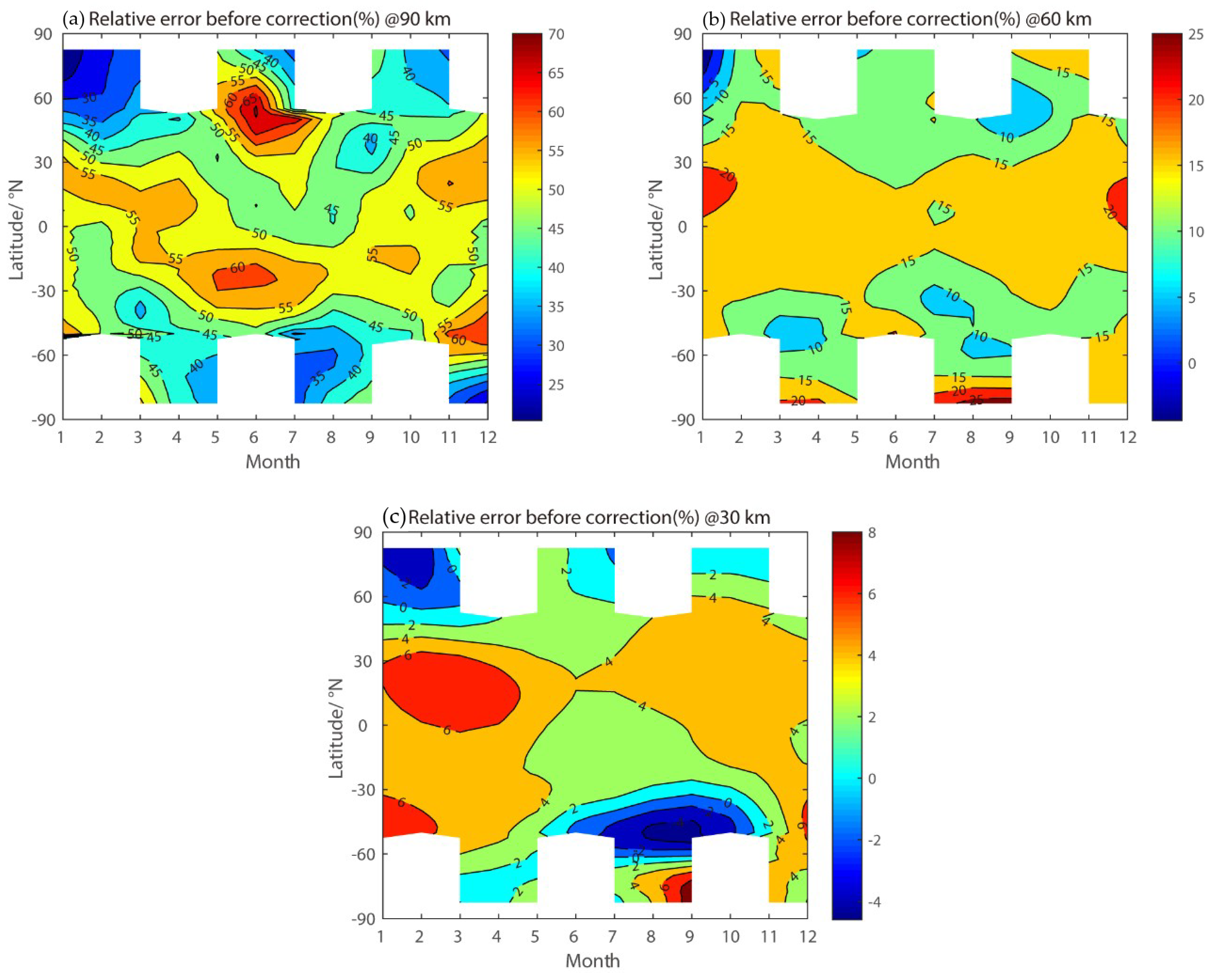
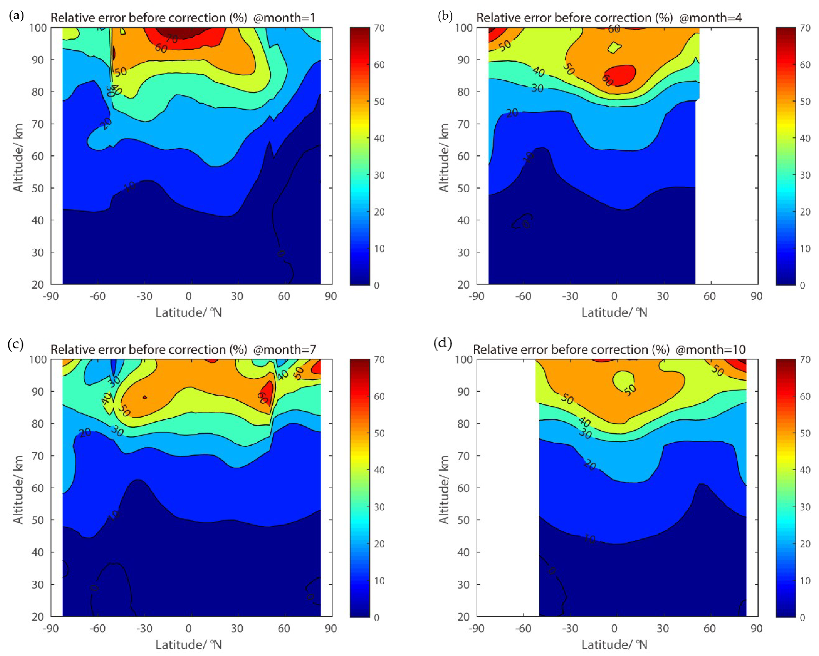
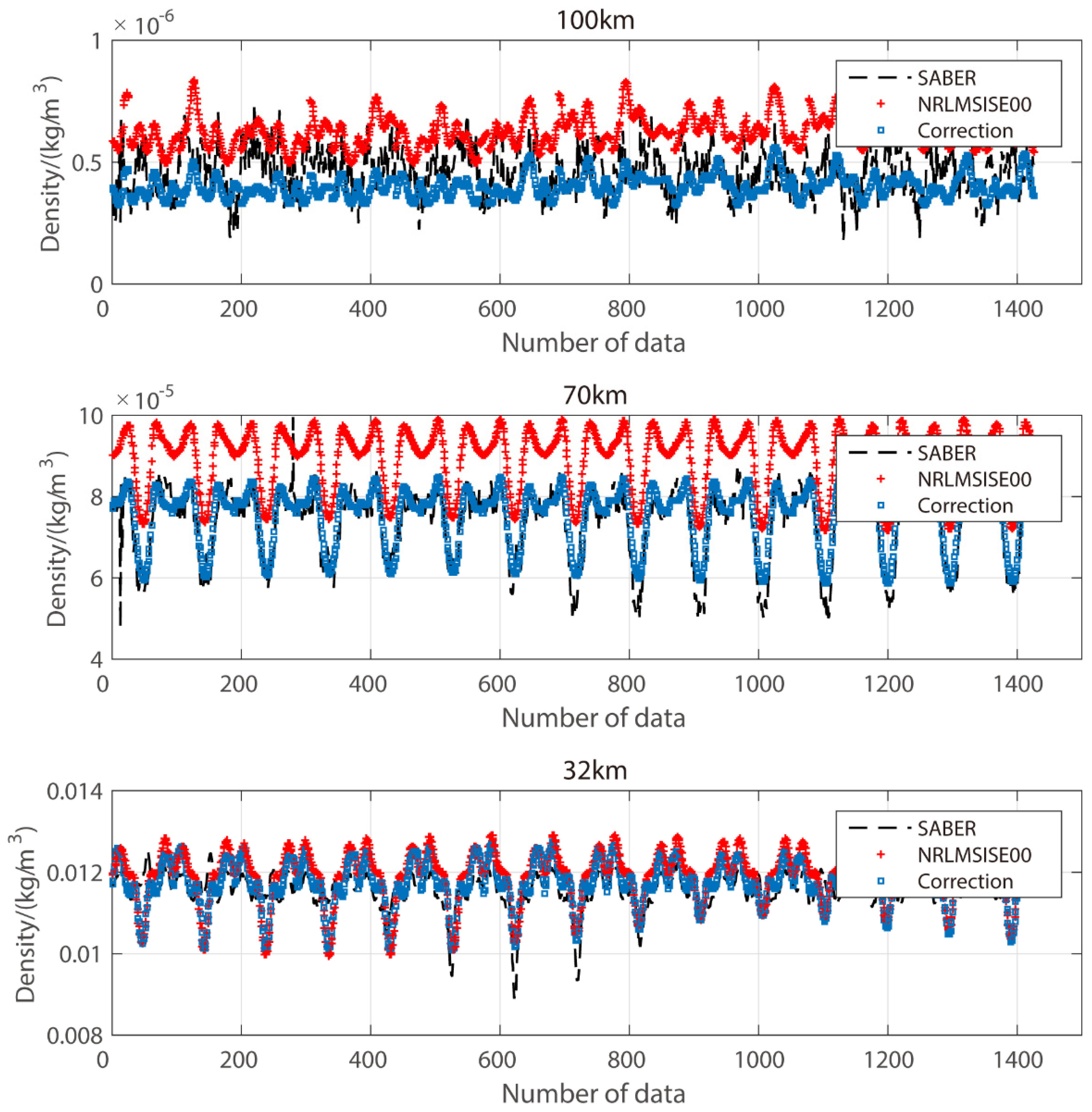
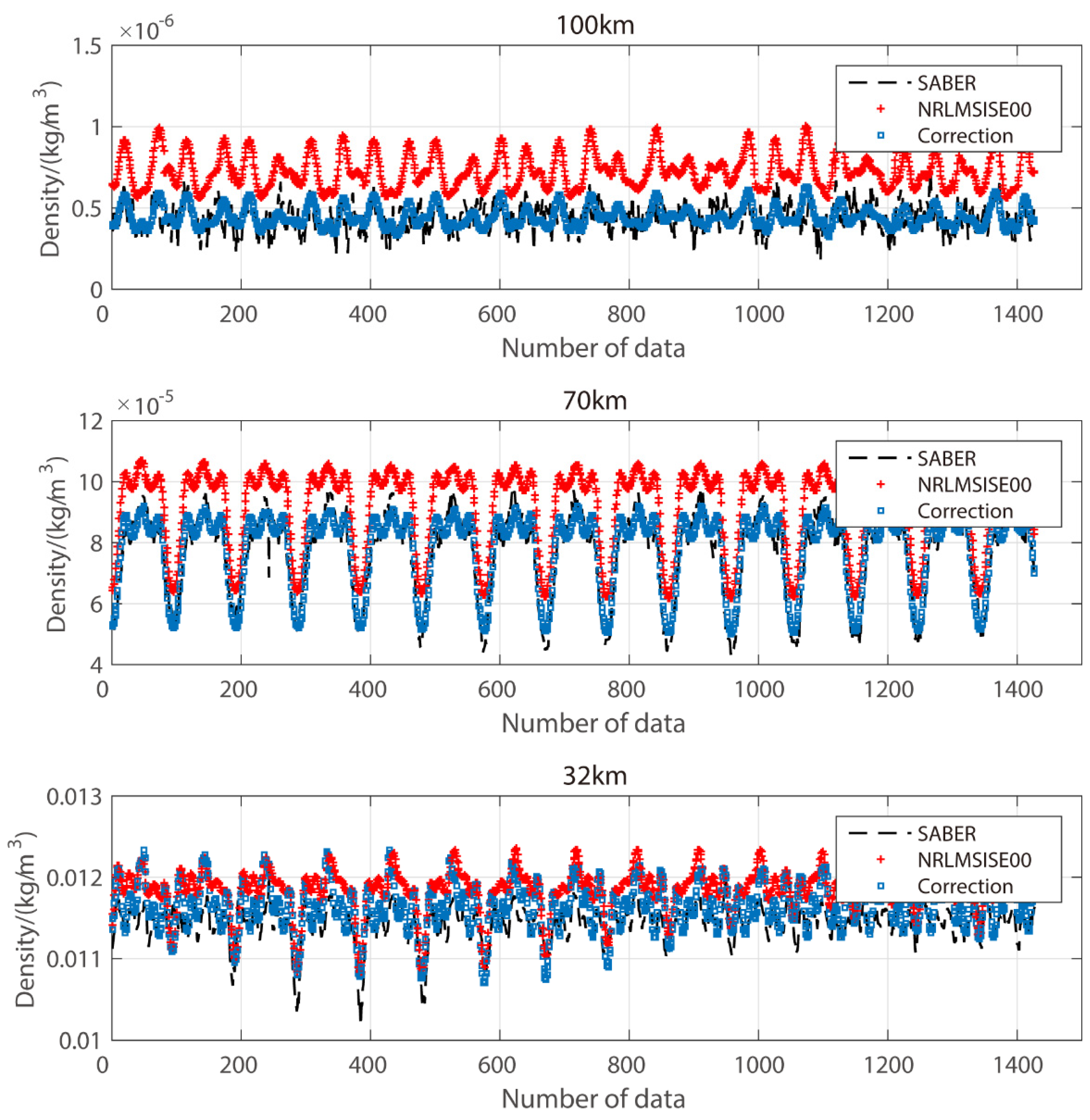
3.1. Difference between Model and Observations

Figure 1 compares the NRLMSISE-00 output with observations. Figure 1a clearly shows the difference between the model and observations at 90 km height. In the vicinity of 60° N and −30° N, the relative error of the model attains maximum values of 68% and 62%, respectively, in June–July. In the vicinity of −60° N and 30° N, the maximum relative error of the model is 63% and 60%, respectively, in December. At 60 km, the relative error of the atmospheric model at low and medium latitudes is mainly around 15%. From December to January, the maximum value of the relative error of the atmospheric model in low latitudes can reach 23%. At 30 km, the relative error maximum value is 7% in the low latitude area from January to April. In the mid-latitudes of the southern hemisphere, there is a minimum value near August, with a relative error of −5%.

As shown in Figure 2, the relative error in model density increases with height for the same latitude. The relative error at middle and low latitudes is higher than that at high latitudes from 80 to 100 km. Near the equator in January, the maximum relative error of the model reaches 79% at 100 km. From 45–80 km, the relative error of the model in the northern hemisphere is greater than that in the northern hemisphere. In July, the relative error is mainly around 50%, with the maximum reaching 68% at 80-100 km. From 45 to 80 km, the relative error of the model at middle and low latitudes in the northern hemisphere is greater than that at high latitudes in the northern hemisphere. In contrast, the relative error of the model at middle and low latitudes in the southern hemisphere is less than that at high latitudes in the southern hemisphere. Below about 45 km, the relative error of the model is generally less than 10%. At 100 km altitude, there are large errors in the model in some regions. The main reason for this deviation is that the NRLMSISE-00 main data source around 100 km is the sounding rocket data of limited stations and limited seasons. These data are insufficient to characterize the atmosphere around 100 km. Therefore, it is reasonable for the model to have such a large deviation at 100 km. Atmospheric planetary waves, atmospheric tidal waves, and atmospheric gravity waves are important sources of atmospheric disturbances above 70 km [31,33,35]. The atmospheric density of NRLMSISE-00 is calculated from the atmospheric temperature. In the UMLT (Upper Mesosphere and Lower Thermosphere) region, there is a large error between the model temperature and the TIMED/SABER observation [36]. The possible reason for the large differences in the UMLT region is that the contributions of propagating planetary waves and gravity waves are not considered in the modeling method of NRLMSISE-00. In addition, inaccurate characterization of atmospheric tides is also a possible reason. The atmospheric model transmits the error caused by the inaccurate representation of the atmospheric temperature disturbance to the atmospheric density, which makes the atmospheric density have larger errors in the UMLT region.

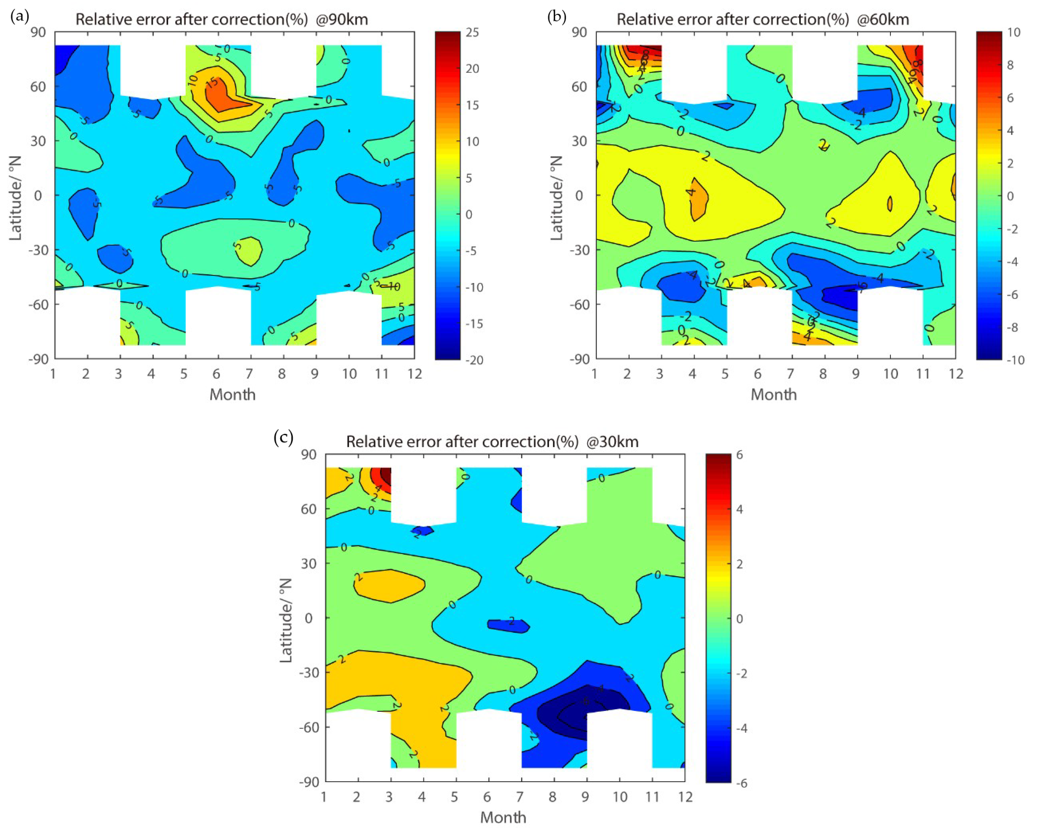
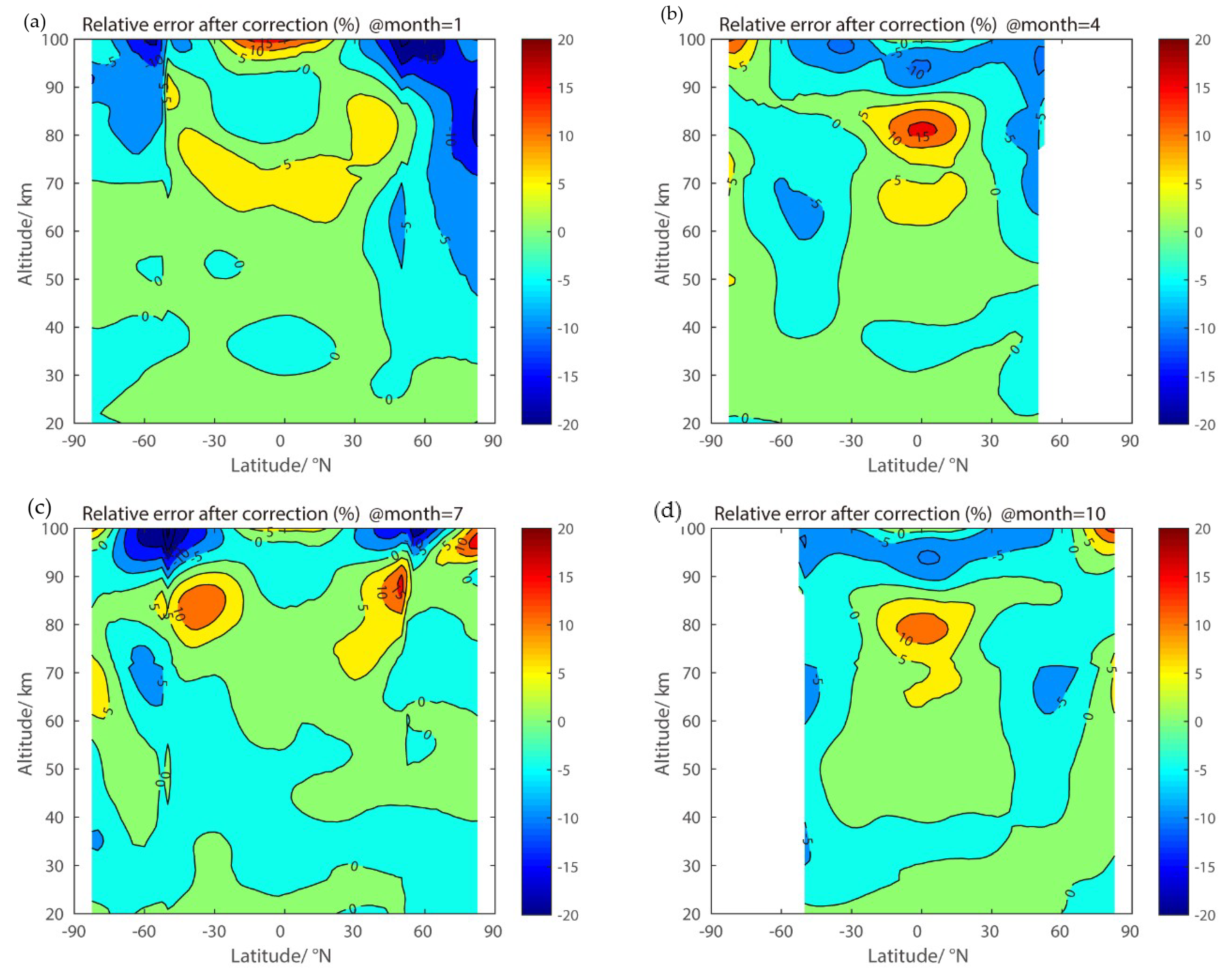
3.2. Statistical Correction Results

3.2.1. Latitude–Month

Using the method described in Section 2.3, the multi-year average relative error of the model density after correction relative to observations is calculated. The results are shown in Figure 3 and Figure 4. Figure 3 shows the latitude–month cross-section of the zonal mean relative error in the calibrated model at different heights. At 90 km, the relative error of the calibrated atmospheric model has a maximum value of 19% near 60° N in June and July. Compared with the relative error of the model before correction, the relative error of the calibrated model reduces the maximum from 68% to 19% in the vicinity of 60° N from June to July. The maximum error decreases from 62% to 7% near −30° N. At 60 km, the relative error of calibrated model reduces the maximum from 23% to less than 4% near the equator in December-January after correction, and in the vicinity of −80°N, the relative error of the calibrated model reduces the maximum from 20% to 3% in April and 26% to 4% in August. At 30 km, the relative error of the calibrated model reduces the maximum from 7% to less than 2% in low latitudes from January to April.

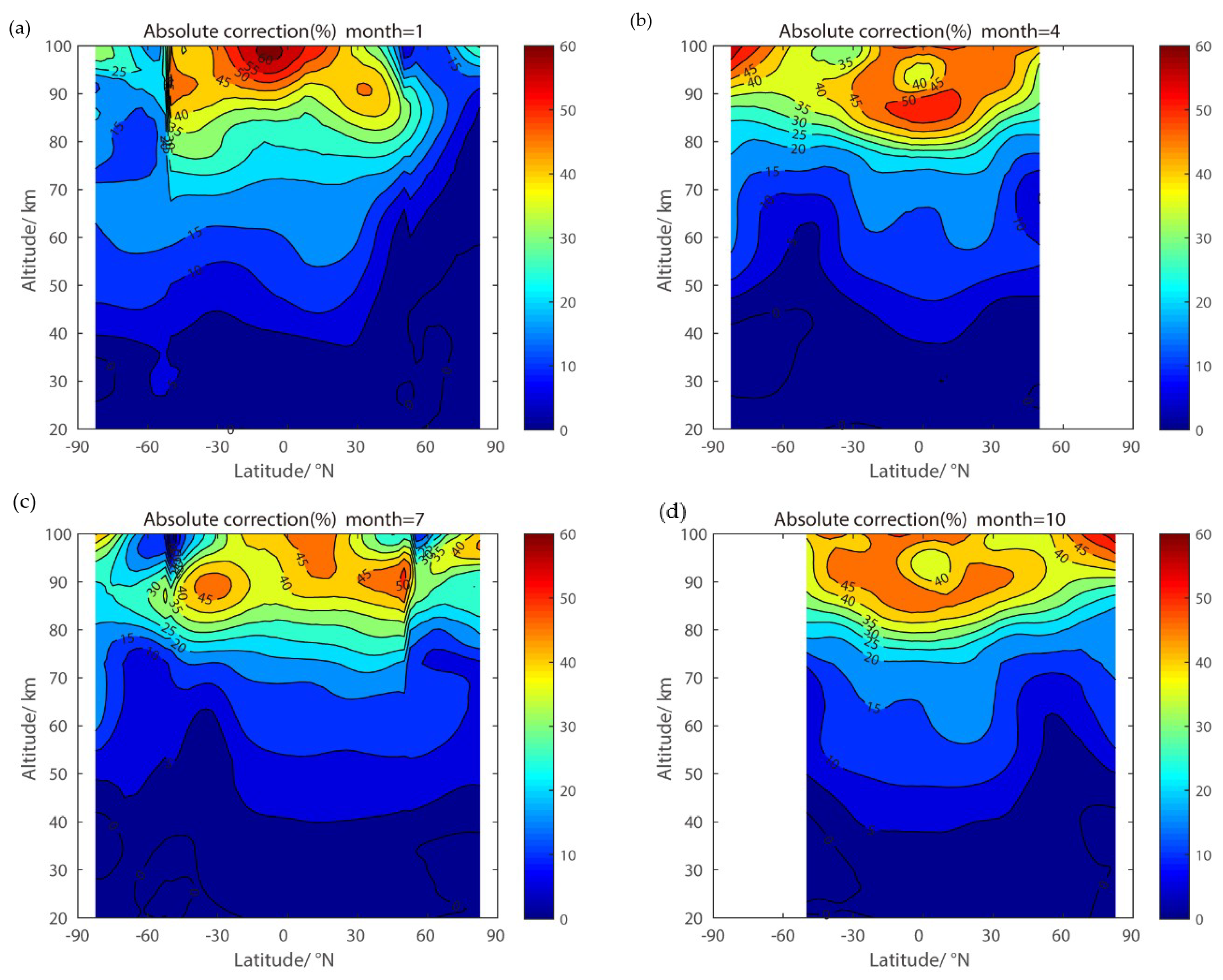
3.2.2. Latitude–Altitudes

Figure 4 shows the latitude–height cross-section of relative deviations in the calibrated model in January, April, July, and October. As it can be seen from the figure, the correction effect of the atmospheric model is significant above 70 km. In January, the relative error of the calibrated model reduces the maximum from 79% to 17% at 100 km near the equator. In April, the relative error of the calibrated model reduces the maximum from 64% to 16% around 80 km near the equator. In July, the maxima occur at ±40°N around 80–90 km, representing relative errors of 14% and 17%. In October, the relative error of the calibrated model has a maximum value of 12% around 80 km. From 20 to 70 km, the relative error of the calibrated model is small. Compared with Figure 2, it can be seen that the relative error between the calibrated data and the observations has been significantly reduced, especially in the middle and low latitudes at heights of 80–100 km.

As can be seen from Figure 3 and Figure 4, there are still some errors after correction. In the correction method of Section 2.2, the existence of the fitting error during the fitting of each component coefficient is one of the possible reasons for the error after correction. In addition, tidal waves also have high-order harmonic components, such as 6 hours, 4 hours, and so on. Only 24, 12, and 8 h tidal components are considered in this paper. The periods of traveling planetary waves are not fixed (e.g., 5, 10, or 16 days), but rather quasi-periodic fluctuations [37,38,39]. In order to simplify the function, we only select a few typical quasi-periodic planetary waves in calculation, and the failure to characterize other possible fluctuations may cause some errors in the correction results.

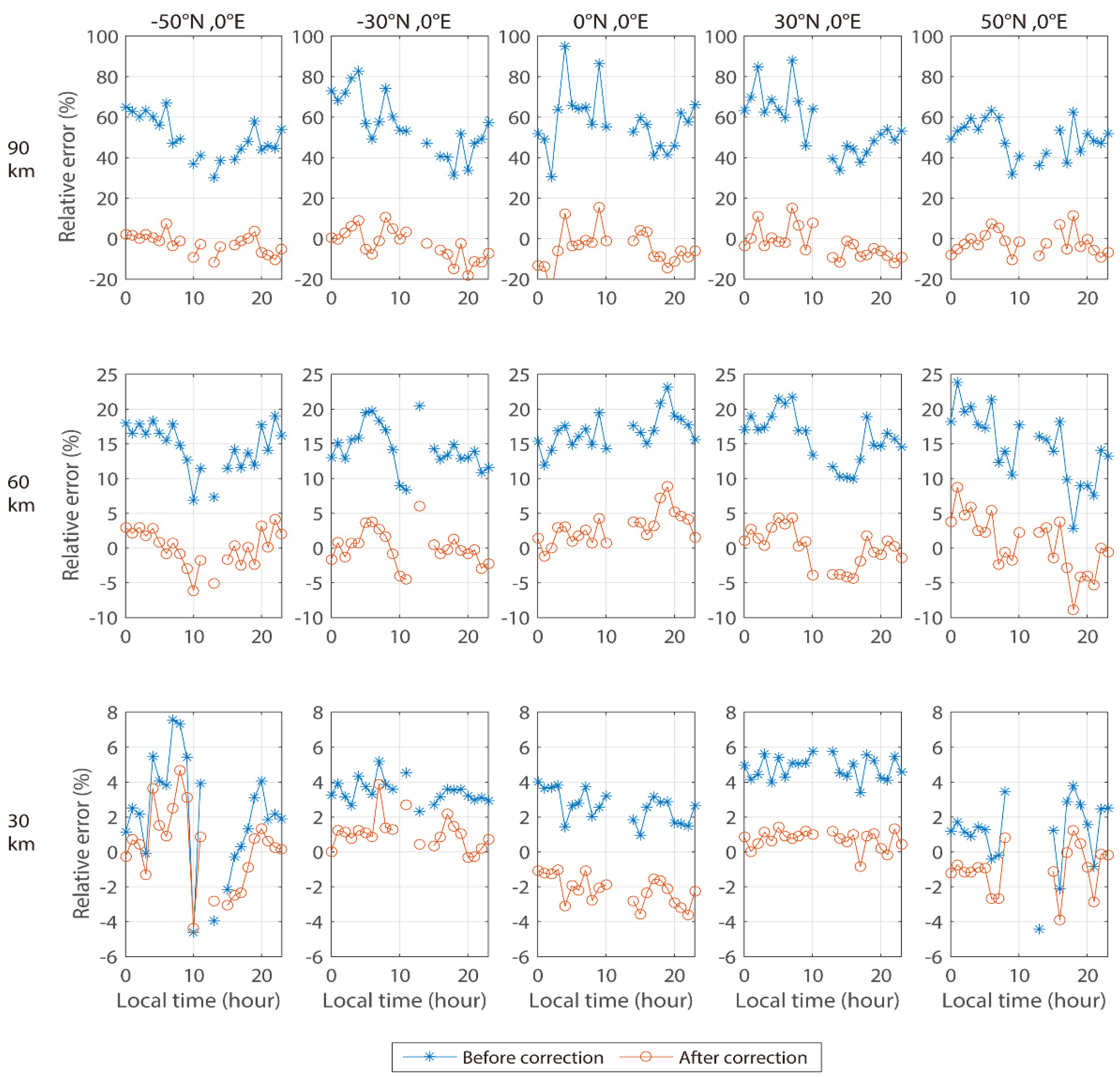
3.3. Correction Results under Different Local Times

In order to compare the correction results of different local times (LT), the relative error is calculated at different local times before and after the correction. Figure 5 shows the relative error of the atmospheric model before and after correction for different local times. At 90 and 60 km, the relative error of the atmospheric model before correction is positive at different geographical locations, indicating that the model values are greater than the satellite observations. At 90 km, the relative error range is between 30% and 100% before correction, and the relative error range is between ±20% after correction. In the latitude of ±50° N, the relative error has a local maximum at about LT 6 and LT 19. The smallest relative error is seen in the LT range of about 10–14, but there is no more data in that LT range. In the latitude of ±30° N, the relative error has a local maximum in the LT range of about 2–7, and there is a local minimum in the LT range of 14–18. At 60 km, the relative error range is mainly between 5% and 25% before correction, and the relative error range is mainly between ±5% after correction.

At 30 km, the relative error of the atmospheric model before correction has both positive and negative values at different local times, and the relative error of the model has improved to some extent. At the same height, the relative error of the atmospheric model varies with local time in the northern hemisphere is similar to that in the southern hemisphere. The relative error varies with local time in a similar sine or cosine function. It can be considered that the relative error has a relationship with the local time, as diurnal waves or semidiurnal waves.

4. Discussion

4.1. Discussion of the Correction Method

Considering the error caused by the inaccurate characterization of atmospheric model density as a result of seasonal variations, intra-annual variations, inter-annual variations, and changes in the 11-year cycle of solar activity, we incorporated the above factors into the correction function. In addition, considering the distribution of atmospheric fluctuations in the atmosphere with height, we divided the range 20–100 km into two height intervals. The first, 70–100 km, contains three height nodes, at 72, 90, and 100 km, whereas the second, 20–70 km, consists of four height nodes, at 20, 32, 45, and 55 km. To simplify the correction function, inaccuracies in the atmospheric tidal characterization were considered in the 70–100 km height interval. As the NRLMSISE-00 does not consider traveling planetary waves, we integrated several traveling planetary wave periodic components into the correction function. At a height of 20–70 km, the atmospheric tide is relatively weak. Below 40 km, the contribution of atmospheric tidal components is small, and the contribution of planetary waves is significant, especially in the winter hemisphere. Therefore, the four height nodes in this interval only consider the atmospheric model to be inaccurate in the representation of planetary waves. To see the correction effect more intuitively, we define the absolute deviation of the relative error between the uncalibrated model and the calibrated model as $∆\mathsf{\delta }=\left|{\delta }_{model}\right|-\left|{\delta }_{correct}\right|$, where $∆\mathsf{\delta }$ is the absolute deviation of the relative error, ${\delta }_{model}$ is the relative error of the model before correction, and ${\delta }_{correct}$ is the relative error of the model after correction. $∆\mathsf{\delta }>0$ indicates that the model density after correction is closer to that observed by SABER, and the corrective effect is considerable. $∆\mathsf{\delta }<0$ indicates that the model density deviates more from the satellite observation of the atmospheric density after correction, i.e., the correction makes the estimate worse. According to Figure 6, the variation in the zonal mean of the model improves in this latitude–altitude cross-section in January, April, July, and October (winter and summer are represented by January and July, and spring and autumn are represented by April and October.) The figure shows that the overall effect of the correction function is significant at 20–100 km, and only the local area model improvement is negative. For example, in the high latitudes of the northern hemisphere in January and the southern hemisphere in April, and the mid-high latitudes of the southern hemisphere in October, the relative error of the corrected model was slightly greater than in the original model. For all areas where the improvement is negative in these months, the results are presented in

Table 1. The average and standard deviations in the area of $∆\delta <0(\%).$

January		April		July		October
Mean	Std	Mean	Std	Mean	Std	Mean	Std
−0.43	0.41	−0.47	0.32	−0.81	0.90	−0.44	0.34

. In the region where $∆\mathsf{\delta }<0$ in January, the average value of the improvement was −0.43%, and the standard deviation was 0.41%. In the region where the improvement is negative, the relative error of the modified model is less than 1% compared with that of the model before correction. In areas where the improvement is negative in other months, the average relative error of the model density before and after correction is again less than 1%. Therefore, the spatiotemporal correction function established in this study has a significant effect on the overall correction of NRLMSISE-00.

4.2. Influence of Geomagnetic Activity

In the correction method, we have not considered the influence of the geomagnetic activity. In order to understand whether the correction effects have some potential relationships with geomagnetic activities, we compared the correction effects under different geomagnetic conditions. Density data from days with an Ap index greater than 80 and less than 27 were selected to calculate the correction effect during a geomagnetic storm and a geomagnetic quiet period, respectively. A large magnetic storm with an Ap index of 106 occurred on September 8, 2017 (day 251), and this was used as the object for evaluating the model during a geomagnetic storm. Most of the days in 2017 were in the geomagnetic quiet period (Ap < 27). The geomagnetic Ap index measured just 5 on 9 May 2017 (day 129) and remained below 10 a few days either side of this day. Thus, the data from 9 May 2017 were selected to evaluate the model during a geomagnetic calm period.

The correction effects were analyzed at three altitude nodes (both node heights and non-node heights were contained), namely 100 km (representing the low thermosphere), 70 km (mesosphere), and 32 km (stratosphere). The density observations from SABER were extracted at these node heights on days 129 and 251. At the same time, the density and corrected density of NRLMSISE-00 were calculated under the same conditions. We then compared the forecast results given by the model before and after correction.

Figure 7 shows the atmospheric density during the geomagnetic storm at 100, 70, and 32 km. There is a large deviation between the atmospheric density calculated by NRLMSISE-00 and that observed by SABER. The corrected model density is closer to the density observed by SABER. The correction effects at 70 and 32 km are considerable.

Table 2. Atmospheric density error on satellite orbits at different nodes on day 251 of 2017 (%).

	100 km		70 km		32 km
	Mean	Std	Mean	Std	Mean	Std
NRLMSISE00	41.21	32.18	22.09	7.74	3.03	4.96
Correction	−9.65	22.56	2.60	5.76	1.44	4.29

presents the statistical results for the relative error in the NRLMSISE-00 density before and after correction on day 251 and the average relative error and standard deviation of the corrected model density. During the geomagnetic storm, the average relative error of NRLMSISE-00 before correction is 41.42%, and the standard deviation is 32.18%. After correction, the average relative error is −9.65%, and the standard deviation is 22.56%. The absolute correction of the model is 31.56%. At 70 km, the average relative error before correction is 22.09%, and the standard deviation is 7.74%. After correction, the average relative error is 2.60%, and the standard deviation is 5.76%. This represents an absolute correction of 19.49%. At 32 km, the average relative error before correction is 3.03%, and the standard deviation is 4.96%. This decreases to an average relative error of 1.44% and the standard deviation of 4.29% after correction, with an absolute correction of 1.59%. Thus, the model is more accurate in characterizing the atmospheric density at these three node heights after error correction.

Figure 8 shows that the density of the three nodes during geomagnetic quiet condition is closer to the SABER observations after correction. The statistical results for the relative error in

Table 3. Atmospheric density error on satellite orbits at different nodes on day 129 of 2017 (%).

	100 km		70 km		32 km
	Mean	Std	Mean	Std	Mean	Std
NRLMSISE00	68.95	33.29	21.02	8.04	3.56	1.57
Correction	3.49	20.65	2.20	6.41	1.77	1.91

indicate that the average relative error before correction is 68.95% with a standard deviation of 33.29% at 100 km. After correction, these values drop to 3.49% and 20.65%, respectively. The absolute correction of the model is 65.46%. Thus, correction significantly improves the accuracy of the density given by NRLMSISE-00 at 100 km in geomagnetic quiet periods. Before correction, the average relative error at 70 km is 21.02%, and the standard deviation is 8.04%. The average relative error decreases to 2.20% with a standard deviation of 6.41% after correction. The absolute correction of the model is 18.82%. Thus, error correction of NRLMSISE-00 makes a considerable improvement in the accuracy of the atmospheric density at 70 km. At a height of 32 km, the average relative error before correction is 3.56%, and the standard deviation is 1.57%. After correction, the average relative error is 1.77%, and the standard deviation of the relative error is 1.91%, with an absolute correction of 1.79%. Again, the model accuracy has been improved by the error correction process.

The comparison results show that the effect of the correction function varies under the different geomagnetic conditions at around 100 km. After correction, the relative error in the model density decreased from 68.95% to 3.49% during a period of geomagnetic quiet condition. During a magnetic storm, the relative error in model density decreased from 41.21% to −9.65%. The correction effect during the geomagnetic quiet condition is better than that during a geomagnetic storm. In addition, the quality of the correction during the geomagnetic storm at 100 km is not so good at the beginning of the day and becomes better towards the end. However, this phenomenon is not observed during the geomagnetic quiet condition. It can be considered that geomagnetic activity may have a potential influence on the correction effect. In this study, the influence of geomagnetic activity is not considered in the process of establishing the correction function due to the unclear response mechanism of middle atmospheric density to geomagnetic activity [40,41,42,43,44]. This factor will be considered in the future to improve the correction ability of the spatiotemporal correction function during magnetic storms and to enhance the model’s ability to represent the real atmosphere.

4.3. Influence of Solar Activity

Solar activity is another important factor in correction factor modeling. The influence of the 11-year cycle of solar activity on atmospheric density is considered in this paper. It is represented by a trigonometric function in the form of the correction factor R of 11-year periodic variation. Here, the solar flux index is not used to build the spatiotemporal function of NRLMSISE-00. From the modeling of temperature, NRLMSISE-00 calculates the density of each component using the physical relationship between the temperature, static equilibrium, and ideal gas state equation. The sum of the density in each of the components is the total density. The response of the NRLMSISE-00 atmospheric density to solar activity depends, to some extent, on the temperature response to solar activity. The sensitivity to solar activity varies with altitude, with studies showing that the effects of solar activity decrease with height. The absorption of solar radiation by ozone in the stratosphere plays an important part in the energy cycle and kinetics of the heating and cooling of the stratosphere. The changes are influenced by kinetics, chemistry, and other parameters [45], while the 11-year solar cycle has little effect on the total ozone content [46]. There are conflicting results regarding the response of MLT to solar activity. Luebken [47] used sounding data to study the structural characteristics of the mesosphere over the polar regions in the past 35 years. The results indicate that the temperature structure of the mesosphere in this zone has not changed significantly. Detailed analysis showed that the solar cycle has little effect on temperature. However, Remsberg and Deaver [48] used HALOE to examine temperature changes in the upper and middle stratosphere from 1991–2004 temperature data. In the upper and middle parts of the tropical stratosphere, the temperature responded significantly to the solar activity week. In the upper part of the tropical stratosphere and the subtropical mesosphere, the trend suggested a linear decline, but this phenomenon has not been found in the tropical mesosphere. Therefore, the mechanism of the influence of solar activity on the middle atmosphere requires further study so that atmospheric models can better characterize the influence of solar activity on the middle atmosphere.

5. Conclusions

In this study, we used density data from TIMED/SABER for the period 2002–2016 to correct the density of the empirical atmospheric model NRLMSISE-00 at a height of 20–100 km for the first time. By analyzing the difference between the model output and the observations, a method for establishing a spatiotemporal correction function for NRLMSISE-00 was proposed. According to the spatiotemporal distribution characteristics of the correction factor dataset, different timescale oscillations in the correction factors appear at every node. The spherical harmonic function was used to fit the coefficients of the separated components to obtain the spatiotemporal correction function for NRLMSISE-00 over the range 20–100 km. The corrected model density was calculated using this function, and the results were evaluated. To this end, the main conclusions from this study are as follows:

(1) The model and observations exhibit the same variation in the horizontal and vertical directions, but there is a certain deviation. The relative error of the model at middle and high latitudes is greater in the summer hemisphere than in the winter hemisphere. In addition, the relative error of the model increases with height in the vertical direction, especially in the region of 80–100 km.

(2) The accuracy of the calibrated model is better than that of NRLMSISE-00. The accuracy of the model is significantly improved at altitudes of 80–100 km, and at different local times, the spatiotemporal correction function also has a significant correction effect on NRLMSISE-00.

(3) The correction effects of the spatiotemporal correction function under different geomagnetic activity are different, and the correction effects may have some potential relationships with geomagnetic activities. The correction effect is better during a geomagnetic calm period. After correction, the relative errors in model density at 100, 70, and 32 km decreased from 41.21%, 22.09%, and 3.03% to −9.65%, 2.60%, and 1.44%, respectively, during a geomagnetic storm. During a geomagnetic quiet period, the relative errors in model density at 100, 70, and 32 km decreased from 68.95%, 21.02%, and 3.56% to 3.49%, 2.20%, and 1.77%, respectively. In the low thermosphere, the correction effect of the function in the geomagnetic calm period is significantly better than that in the magnetic storm period. Subsequent work will consider the effects of geomagnetic activity and optimize the ability of the spatiotemporal correction function to correct the atmospheric density during magnetic storms.

The density mechanism in response to solar activity and geomagnetic activity requires further investigation in the range 20–100 km. This theoretical study provides a technical basis for the establishment of new models and the improvement of existing models and enhances the ability of NRLMSISE-00 to represent the real atmosphere. By correcting the density over the range 20–100 km for NRLMSISE-00, higher-quality initial and background fields can be provided for numerical simulations and predictions in scientific research. Additionally, reliable atmospheric density data can be derived for aircraft design, simulation, and flight tests in aerospace and other engineering fields.

References

1. Huang, R.; Chen, W.; Wei, K.; Wang, L.; Huangfu, J. Atmospheric dynamics in the stratosphere and its interaction with tropospheric processes: Progress and problems. Chin. J. Atmos. Sci. 2018, 42, 463–487. [Google Scholar] [CrossRef]
2. Matsuno, T. Vertical Propagation of Stationary Planetary Waves in the Winter Northern Hemisphere. J. Atmos. Sci. 1970, 27, 871–883. [Google Scholar] [CrossRef] [Green Version]
3. Alexander, J. A Simulated Spectrum of Convectively Generated Gravity Waves: Propagation from the Tropopause to the Mesopause and Effects on the Middle Atmosphere. J. Geophys. Res. 1996, 101, 1571–1588. [Google Scholar] [CrossRef]
4. Semeniuk, K.; Fomichev, V.I.; McConnell, J.C.; Fu, C.; Melo, S.M.L.; Usoskin, I.G. Middle atmosphere response to the solar cycle in irradiance and ionizing particle precipitation. Atmos. Chem. Phys. 2011, 11, 5045–5077. [Google Scholar] [CrossRef] [Green Version]
5. Rozanov, E.; Calisto, M.; Egorova, T.; Peter, T.; Schmutz, W. Influence of the Precipitating Energetic Particles on Atmospheric Chemistry and Climate. Surv. Geophys. 2012, 33, 483–501. [Google Scholar] [CrossRef] [Green Version]
6. Kim, J.S.; Urbina, J.V.; Kane, T.J.; Spencer, D.B. Improvement of TIE-GCM thermospheric density predictions via incorporation of helium data from NRLMSISE-00. J. Atmos. Sol. Terr. Phys. 2012, 77, 19–25. [Google Scholar] [CrossRef]
7. Namgaladze, A.A.; Zubova, Y.V.; Namgaladze, A.N.; Martynenko, O.V.; Doronina, E.N.; Goncharenko, L.P.; Van Eyken, A.; Howells, V.; Thayer, J.P.; Taran, V.I.; et al. Modelling of the ionosphere/thermosphere behaviour during the April 2002 magnetic storms: A comparison of the UAM results with the ISR and NRLMSISE-00 data. Adv. Space Res. 2006, 37, 380–391. [Google Scholar] [CrossRef]
8. Park, J.; Moon, Y.J.; Kim, K.H.; Cho, K.S.; Kim, H.D.; Kwak, Y.S.; Kim, Y.H.; Park, Y.D.; Yi, Y. Comparison between the KOMPSAT-1 drag derived density and the MSISE model density during strong solar and/or geomagnetic activities. EarthPlanets Space 2008, 60, 601–606. [Google Scholar] [CrossRef] [Green Version]
9. Qian, L.Y.; Burns, A.G.; Solomon, S.S.; Smith, A.K.; McInerney, J.M.; Hunt, L.A.; Marsh, D.R.; Liu, H.L.; Mlynczak, M.G.; Vitt, F.M. Temporal Variability of Atomic Hydrogen From the Mesopause to the Upper Thermosphere. J. Geophys. Res. Space 2018, 123, 1006–1017. [Google Scholar] [CrossRef]
10. Yurasov, V.S.; Nazarenko, A.I.; Alfriend, K.T.; Cefola, P.J. Reentry time prediction using atmospheric density corrections. J. Guid. Control Dynam. 2008, 31, 282–289. [Google Scholar] [CrossRef]
11. Chen, H.R.; Liu, H.X.; Hanada, T. Storm-time atmospheric density modeling using neural networks and its application in orbit propagation. Adv. Space Res. 2014, 53, 558–567. [Google Scholar] [CrossRef]
12. Lathuillère, C.; Menvielle, M. Comparison of the observed and modeled low- to mid-latitude thermosphere response to magnetic activity: Effects of solar cycle and disturbance time delay. Adv. Space Res. 2010, 45, 1093–1100. [Google Scholar] [CrossRef]
13. Vielberg, K.; Forootan, E.; Luck, C.; Locher, A.; Kusche, J.; Borger, K. Comparison of accelerometer data calibration methods used in thermospheric neutral density estimation. Ann. Geophys. Ger. 2018, 36, 761–779. [Google Scholar] [CrossRef] [Green Version]
14. Xu, J.; Qiao, J.; Wei, Y.; Ruiping, M. Comparison between the TIMED observed global temperature distribution and the NRLMSISE-00 empirical atmospheric model. Chin. J. Space Sci. 2006, 26, 177–182. [Google Scholar]
15. Zhou, Y.L.; Ma, S.Y.; Lühr, H.; Xiong, C.; Reigber, C. An empirical relation to correct storm-time thermospheric mass density modeled by NRLMSISE-00 with CHAMP satellite air drag data. Adv. Space Res. 2009, 43, 819–828. [Google Scholar] [CrossRef]
16. Picone, J.M.; Hedin, A.E.; Drob, D.P.; Aikin, A.C. NRLMSISE-00 empirical model of the atmosphere: Statistical comparison and scientific issues. J. Geophys. Res. 2002, 107, 1468. [Google Scholar] [CrossRef]
17. Bergstrom, S.E.; Proulx, R.J.; Cefola, P. Atmospheric density correction using observational data. In Proceedings of the AIAA/AAS Astrodynamics Specialist Conference and Exhibit, Monterey, CA, USA, 5–8 August 2002. [Google Scholar]
18. Chen, X.; Hu, X.; Xiao, C.; Wang, X. Correction method of the low earth orbital neutral density prediction based on the satellites data and NRLMSISE-00 model. Chin. J. Geophys. 2013, 56, 3246–3254. [Google Scholar] [CrossRef]
19. Shi, C.; Li, W.; Min, L.; Zhao, Q.; Sang, J. Calibrating the scale of the NRLMSISE00 model during solar maximum using the two line elements dataset. Adv. Space Res. 2015, 56, 1–9. [Google Scholar] [CrossRef]
20. Mehta, P.M.; Linares, R. A methodology for reduced order modeling and calibration of the upper atmosphere. Space Weather 2017, 15, 1270–1287. [Google Scholar] [CrossRef]
21. Zhang, H.; Gu, D.; Duan, X.; Wei, C. Atmospheric density model calibration using emperical orthogonal function. Acta Aeronaut. Astronaut. Sin. 2018, 39, 722263. [Google Scholar] [CrossRef]
22. Perez, D.; Bevilacqua, R. Neural Network based calibration of atmospheric density models. Acta Astronaut. 2015, 110, 58–76. [Google Scholar] [CrossRef]
23. Xiong, C.; Lühr, H.; Schmidt, M.; Bloßfeld, M.; Rudenko, S. An empirical model of the thermospheric mass density derived from CHAMP satellite. Ann. Geophys. Ger. 2018, 36, 1141–1152. [Google Scholar] [CrossRef] [Green Version]
24. Emmert, J.T. Thermospheric mass density: A review. Adv. Space Res. 2015, 56, 773–824. [Google Scholar] [CrossRef]
25. Mertens, C.; Russell, J., III; Mlynczak, M.; She, C.-Y.; Schmidlin, F.J.; Goldberg, R.; López-Puertas, M.; Wintersteiner, P.P.; Picard, R.; Winick, J.; et al. Kinetic temperature and carbon dioxide from broadband infrared limb emission measurements taken from the TIMED/SABER instrument. Adv. Space Res. 2009, 43, 15–27. [Google Scholar] [CrossRef] [Green Version]
26. Russell, J.M.; Mlynczak, M.G.; Gordley, L.L.; Tansock, J.; Esplin, R. An overview of the SABER experiment and preliminary calibration results. Opt. Spectrosc. Tech. Instrum. Atmos. Space Res. III 1999, 3756, 277–288. [Google Scholar] [CrossRef] [Green Version]
27. Remsberg, E.E.; Marshall, B.T.; Garcia-Comas, M.; Krueger, D.; Lingenfelser, G.S.; Martin-Torres, J.; Mlynczak, M.G.; Russell, J.M.; Smith, A.K.; Zhao, Y.; et al. Assessment of the quality of the Version 1.07 temperature-versus-pressure profiles of the middle atmosphere from TIMED/SABER. J. Geophys. Res. 2008, 113, D17101. [Google Scholar] [CrossRef]
28. Rezac, L.; Kutepov, A.; Russell Iii, J.; Feofilov, A.; Yue, J.; Goldberg, R. Simultaneous retrieval of T(p) and CO2 VMR from two-channel non-LTE limb radiances and application to daytime SABER/TIMED measurements. J. Atmos. Sol. Terr. Phys. 2015, 130–131, 23–42. [Google Scholar] [CrossRef]
29. Gong, X.Y.; Hu, X.; Wu, X.C.; Xiao, C.Y. Comparison of temperature measurement between COSMIC atmospheric radio occultation and SABER/TIMED (in Chinese). Chin. J. Geophys. 2013, 56, 2152–2162. [Google Scholar] [CrossRef]
30. Xu, J.; She, C.Y.; Wei, Y.; Mertens, C.; Mlynczak, M.; Russell, J. Comparison between the temperature measurements by TIMED/SABER and lidar in the midlatitude. J. Geophys. Res. Space Phys. 2006, 111, A10S09. [Google Scholar] [CrossRef]
31. Xiao, C.Y.; Hu, X.; Wang, B.; Yang, J.F. Quantitative studies on the variations of near space atmospheric fluctuation. Chin. J. Geophys. 2016, 59, 1211–1221. [Google Scholar] [CrossRef]
32. Xiao, C.Y.; Hu, X.; Yang, J.F.; Yan, Z.A.; Liu, T.; Cheng, X. Characteristics of atmospheric density at 38° N in near space and its modeling technique. J. Beijing Univ. Aeronaut. Astronaut. 2017, 43, 1757–1765. [Google Scholar] [CrossRef]
33. Pancheva, D.; Mukhtarov, P. Atmospheric Tides and Planetary Waves: Recent Progress Based on SABER/TIMED Temperature Measurements (2002–2007). In Aeronomy of the Earth’s Atmosphere and Ionosphere; Springer: Dordrecht, The Netherlands, 2011; pp. 19–56. [Google Scholar] [CrossRef]
34. Xu, J.; Smith, A.K.; Yuan, W.; Liu, H.; Wu, Q.; Mlynczak, M.G. The Global Structure and Long Term Variations of the Temperature Observed by TIMED/SABER. J. Geophys. Res. 2006, 112, D24106. [Google Scholar] [CrossRef] [Green Version]
35. Zhang, X.; Forbes, J.M.; Hagan, M.E.; Russell, J.M.; Palo, S.E.; Mertens, C.J.; Mlynczak, M.G. Monthly tidal temperatures 20–120 km from TIMED/SABER. J. Geophys. Res. 2006, 111. [Google Scholar] [CrossRef]
36. Xuan, C.; Cunying, X.; Xiong, H.; Junfeng, Y. Evaluation of atmospheric empirical model based on TIMED/SABER satellite temperature data. Sci. Sin. Phys. Mech. Astron. 2018, 48, 79–93. [Google Scholar] [CrossRef]
37. Day, K.A.; Mitchell, N.J. The 16-day wave in the Arctic and Antarctic mesosphere and lower thermosphere. Atmos. Chem. Phys. 2010, 115. [Google Scholar] [CrossRef] [Green Version]
38. Nielsen, K.; Siskind, D.E.; Eckermann, S.D.; Hoppel, K.W.; Coy, L.; McCormack, J.P.; Benze, S.; Randall, C.E.; Hervig, M.E. Seasonal variation of the quasi 5 day planetary wave: Causes and consequences for polar mesospheric cloud variability in 2007. J. Geophys. Res. Atmos. 2010, 115. [Google Scholar] [CrossRef] [Green Version]
39. Pancheva, D.; Mukhtarov, P.; Siskind, D.E. The quasi-6-day waves in NOGAPS-ALPHA forecast model and their climatology in MLS/Aura measurements (2005–2014). J. Atmos. Sol. Terr. Phys. 2018, 181, 19–37. [Google Scholar] [CrossRef]
40. Lei, J.; Thayer, J.; Forbes, J.M.; Sutton, E.K.; Nerem, R.; Temmer, M.; Veronig, A. Global thermospheric density variations caused by high-speed solar wind streams during the declining phase of solar cycle 23. J. Geophys. Res. 2008, 113, A11303. [Google Scholar] [CrossRef]
41. Mengistu Tsidu, G.; Abraha, G. Moderate geomagnetic storms of January 22–25, 2012 and their influences on the wave components in ionosphere and upper stratosphere-mesosphere regions. Adv. Space Res. 2014, 54, 1793–1812. [Google Scholar] [CrossRef]
42. Xu, J.; Wang, W.; Zhang, S.-R.; Liu, X.; Yuan, W. Multiday thermospheric density oscillations associated with variations in solar radiation and geomagnetic activity: Thermospheric density oscillations. J. Geophys. Res. Space Phys. 2015, 120, 3829–3846. [Google Scholar] [CrossRef]
43. Yi, W.; Reid, I.; Xue, X.; Murphy, D.J.; Hall, C.M.; Tsutsumi, M.; Ning, B.; Li, G.; Younger, J.P.; Chen, T.; et al. High- and Middle-Latitude Neutral Mesospheric Density Response to Geomagnetic Storms. Geophys. Res. Lett. 2018, 45, 436–444. [Google Scholar] [CrossRef] [Green Version]
44. Yi, W.; Reid, I.; Xue, X.; Younger, J.P.; Murphy, D.J.; Chen, T.; Dou, X. Response of neutral mesospheric density to geomagnetic forcing. Geophys. Res. Lett. 2017, 44, 8647–8655. [Google Scholar] [CrossRef] [Green Version]
45. Staehelin, J.; Harris, N.R.; Appenzeller, C.; Eberhard, J. Ozone trends: A review. Rev. Geophys. 2001, 39, 231–290. [Google Scholar] [CrossRef] [Green Version]
46. Hood, L.L. The solar cycle variation of total ozone: Dynamical forcing in the lower stratosphere. J. Geophys. Res. 1997, 102, 1355–1370. [Google Scholar] [CrossRef] [Green Version]
47. Luebken, F.-J. No long term change of the thermal structure in the mesosphere at high latitudes during summer. Adv. Space Res. 2001, 28, 947–953. [Google Scholar] [CrossRef]
48. Remsberg, E.E.; Deaver, L.E. Interannual, solar cycle, and trend terms in middle atmospheric temperature time series from HALOE. J. Geophys. Res. Atmos 2005, 110, D06106. [Google Scholar] [CrossRef] [Green Version]
Figure 1. The latitude versus month variations of zonal mean relative difference between NRLMSISE-00 and TIMED/SABER density before correction at (a) 90, (b) 60, and (c) 30 km.
Atmosphere 11 00341 g001
Figure 2. The latitude versus height variations of zonal mean relative difference between NRLMSISE-00 and TIMED/SABER density before correction in (a) January, (b) April, (c) July, (d) October.
Atmosphere 11 00341 g002
Figure 3. Same as Figure 1 but for zonal mean relative difference between NRLMSISE-00 and TIMED/SABER density after correction at (a) 90, (b) 60, and (c) 30 km.
Atmosphere 11 00341 g003
Figure 4. Same as Figure 2 but for zonal mean relative difference between NRLMSISE-00 and TIMED/SABER density after correction in (a) January, (b) April, (c) July, (d) October.
Atmosphere 11 00341 g004
Figure 5. The relative error between NRLMSISE-00 and TIMED/SABER density before and after correction varies with local time in 2008. The blue line refers to the relative error before correction. The red line refers to the relative error after correction.
Atmosphere 11 00341 g005
Figure 6. Latitude–height cross-section of δ in (a) January, (b) April, (c) July, and (d) October. δ = | δ m o d e l | | δ c o r r e c t | . δ > 0 indicates that the corrective effect is considerable; δ < 0 indicates that the correction makes the estimate worse.
Atmosphere 11 00341 g006
Figure 7. Density variations at different heights during a geomagnetic storm (day 251 of 2017) at 100, 70, 32 km. The black line refers to TIMED/SABER density. The red asterisk refers to NRLMSISE-00 density before correction. The blue square refers to NRLMSISE-00 density after correction.
Atmosphere 11 00341 g007
Figure 8. Same as Figure 7 but for day 129 of 2017.
Atmosphere 11 00341 g008