Shallow Water Magnetohydrodynamics in Plasma Astrophysics. Waves, Turbulence, and Zonal Flows

Abstract

The purpose of plasma astrophysics is the study and description of the flow of rotating plasma in order to understand the evolution of various objects in the universe, from stars and planetary systems to galaxies and galaxy clusters. A number of new applications and observations have appeared in recent years and actualized the problem of studying large-scale magnetohydrodynamic flows, such as a thin layer under the convective zone of the sun (solar tachocline), propagation of accreting matter in neutron stars, accretion disks in astrophysics, dynamics of neutron star atmospheres, and magnetoactive atmospheres of exoplanets tidally locked with their host star. The article aims to discuss a fundamental problem in the description and study of multiscale astrophysical plasma flows by studying its general properties characterizing different objects in the universe. We are dealing with the development of geophysical hydrodynamic ideas concerning substantial differences in plasma flow behavior due to the presence of magnetic fields and stratification. We discuss shallow water magnetohydrodynamic equations (one-layer and two-layer models) and two-dimensional magnetohydrodynamic equations as a basis for studying large-scale flows in plasma astrophysics. We discuss the novel set of equations in the external magnetic field. The following topics will be addressed: Linear theory of magneto-Rossby waves, three-wave interactions and related parametric instabilities, zonal flows, and turbulence.

1. Introduction

Plasma in various stars and planets is described by the magnetohydrodynamics of a thin fluid layer with a free surface in the gravity field. As an example we refer to solar tachocline flows (a thin layer inside the sun located at the bottom of the convection zone) [1,2,3,4,5,6,7,8,9], neutron star atmosphere dynamics [10,11], accreting matter flows in neutron stars [12], and tidally synchronized exoplanets with magnetoactive atmospheres [13,14,15,16]. Such thin layer flows of astrophysical plasma are described by the magnetohydrodynamic (MHD) shallow water approximation [17] and two-dimensional MHD approximation [17,18,19]. The advantage of shallow water approximation is the ability to take into account the vertical magnetic field while two-dimensional (2D) MHD approximation is more suitable for turbulence studies [18,20,21].

The MHD equations in shallow water approximation are the alternative for heavy fluid MHD equations in a case where the layer of incompressible inviscid plasma in a gravity field with a free surface is considered. The non-inertial reference frame is rotating with the plasma layer. The MHD shallow water equations are obtained by height-averaging general incompressible MHD equations. The pressure is assumed to be hydrostatic and layer height is assumed to be much smaller than is characteristic for a horizontal linear scale of plasma layer [17,22,23,24,25,26,27,28,29,30]. The obtained equations play an important role in astrophysical plasma studies as do the classical shallow water equations in neutral fluid hydrodynamics. Here, we deal with MHD shallow water equations in the external vertical magnetic field [10,30]. Such a configuration of a magnetic field is typical for neutron stars [10,16] and exoplanets [16]. The presence of the external magnetic field leads to new types of waves: Magneto-Poincare waves and magnetostrophic waves. A detailed analysis of magneto-Poincare and magnetostrophic three-wave interactions and related parametric instabilities is given in [30,31].

The next step is taking into account the effects of stratification. Astrophysical plasma flows tend to be stratified, but a complete system of magnetohydrodynamic equations of stratified plasma in an external field is too complicated for theoretical analysis. The model of superimposed n layers of different densities is one of many useful models for stratified plasma [28,32]. Here, equations obtained in [30,31,33] are generalized to the case of a thin plasma layer divided into two layers with different densities [34]. Obtained MHD two-layer shallow water equations include an external vertical magnetic field and stratification and play the same important role in astrophysical stratified plasma as the classical shallow water equations in the neutral stratified fluid dynamics [35]. In [36] the linear analysis of the magnetohydrodynamic flows under the Boussinesq approximation leads to the magneto-Archimdes Coriolis waves which are similar to the shallow water magnetohydrodynamic waves on a f-plane. Taking into account the stratification in MHD models of rotating plasma is important for the analysis of R-mode oscillations in rotating stars and in the sun [37,38,39], and significantly increases the possibility for interpreting the available observational data for large-scale Rossby waves in the sun [40,41,42,43]. The $\beta$-plane approximation is used to describe the dynamics of a plasma layer in the presence of the differential rotation and allows to consider the effects of spherical geometry [30]. In $\beta$-plane approximation, it is assumed that the Coriolis parameter $f=2\Omega sin\theta$ ($\Omega$—angular velocity, $\theta$—latitude) can be expanded in a series up to the first order of smallness near local latitude. Rossby waves play an important role in the formation of zonal flows in two-dimensional magnetohydrodynamic turbulence [21]. Magnetic Rossby waves obtained in [1,40] are observed in the sun [39,43] and explain solar seasons [8,41,42]. Magneto-Rossby waves determine the large-scale dynamics of the sun and stars, magnetoactive atmospheres of tidally locked exoplanets, flows in accretion disks, and in atmospheres of neutron stars.

As was mentioned above, plasma flows are usually stratified. Thus, the study of stratification in the theory of linear Rossby waves in frameworks of the MHD two-layer shallow water model is of significant importance. In this paper, the multiscale method is used to analyze nonlinear interactions of magneto-Rossby waves and three-wave nonlinear amplitude equations [33,34]. It is shown that there are two types of instabilities and their growth rates are found. Below we give important details of the MHD one-layer and two-layer shallow water models as well as recent advances in theory of non-linear interactions of magneto-Rossby waves on the basis of our previous research [30,31,33,34].

The equations of two-dimensional magnetohydrodynamics with the Coriolis force in a $\beta$-plane approximation are used for a qualitative analysis and numerical simulation of processes in plasma astrophysics. Two-dimensional equations allow a solution in the form of Rossby waves in the linear approximation, whereas in the nonlinear limit, these equations in the absence of the $\beta$-term describe classical isotropic two-dimensional MHD turbulence. The complete equations of two-dimensional magnetohydrodynamics on a $\beta$-plane describe the interaction of two-dimensional MHD turbulence and Rossby waves. We also note that 2D MHD equations on a $\beta$-plane have a solution in the form of magneto-Rossby waves in the presence of poloidal and/or toroidal magnetic field in the linear approximation [33], turbulent flows with Alfven waves in the nonlinear limit without the $\beta$-effect, and their interaction in the complete system of equations. This situation is typical for the solar tachocline [18].

MHD turbulence in a rotating plasma is a common state of flow in plasma astrophysics. The study of fundamental properties of turbulence allows one to understand the evolution of various astrophysical objects from the sun and stars to planetary systems, galaxies, and galaxy clusters. This study requires the generalization and development of methods of geophysical fluid dynamics [44] taking into account fundamental differences in the behavior of large-scale turbulent plasma flows in the presence of magnetic fields. A solution of such a complex physical problem requires both the development of simplified models and the use of numerical experiments. This particularly concerns zonal flows appearing because of isotropy breaking in the system due to two anisotropization mechanisms in astrophysical plasma, namely, rotation and Lorentz force. Thus, the picture of zonal flows characteristic of planetary atmospheres [45,46,47,48] becomes more complicated.

Zonal flows in magnetohydrodynamics are also typical for a toroidal plasma. Stationary solutions for the toroidal magnetized plasma in the form of shear flows along magnetic surfaces were found in [49,50]. The formation of zonal flows in such systems is attributed to drift turbulence [51].

Below, first results on space-time dynamics of two-dimensional rotating decaying MHD turbulence and zonal flows physics are outlined based on [21]. Qualitative concepts on the determination of the boundary between wave and turbulent dynamics are generalized for a MHD case and a new criterion is suggested describing the boundary between wave dynamics and MHD turbulence [21,52]. This is a promising field of research because it is well known that even a very low magnetic field can play an important role, changing the properties of turbulent transport in a conducting fluid. The model of 2D MHD turbulence in the presence of the Coriolis force is a base model in plasma astrophysics, since flows tend to become plane due to fast rotation or the effect of an external vertical magnetic field [53]. It is also noteworthy that, in the presence of strong stratification, turbulent flows demonstrate the formation of numerous planar structures in the form of two-dimensional non-interacting layers. Most (not all) flows in plasma astrophysics have a spherical geometry therefore, the projection of the angular rotation velocity on the local vertical coordinates varies with the latitude. The $\beta$-plane approximation is used for the linear approximation of the Coriolis parameter f dependence on the coordinate in the south-north direction. Below, first results of numerical simulation of two-dimensional decaying MHD turbulence on the $\beta$-plane are presented based on [21].

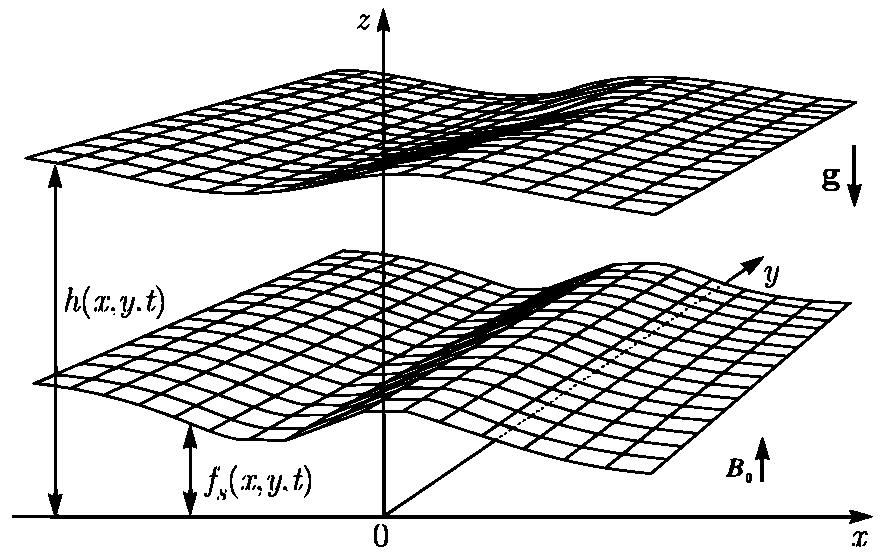
2. Magnetohydrodynamic Shallow Water Equations With an External Field in Rotating Frame: Magneto-Rossby Waves

In this section we briefly discuss the details of a shallow water MHD model in an external vertical magnetic field and recent findings of linear magneto-Rossby waves and their non-linear interactions [10,30,31,33]. The MHD shallow water equations in an external vertical magnetic field are obtained from the full set of three-dimensional MHD equations. These shallow water equations are obtained for the thin fluid layer with a free surface in the gravitational field (Figure 1) which is rotating with the Coriolis parameter f [10]. For a magnetic field normalized by the factor ${(4\pi \rho )}^{-\frac{1}{2}}$, in which $\rho$ is the (assumed constant) density the equations take the form:

$$\frac{\partial h}{\partial t}+\frac{\partial h{v}_x}{\partial x}+\frac{\partial h{v}_y}{\partial y}=0$$

(1)

$$\frac{\partial \left(h{v}_x\right)}{\partial t}+\frac{\partial \left(h(v_x^2-B_x^2)\right)}{\partial x}+gh\frac{\partial h}{\partial x}+\frac{\partial \left(h(v_x{v}_y-B_x{B}_y)\right)}{\partial y}+B_0{B}_x=fh{v}_y$$

(2)

$$\frac{\partial \left(h{v}_y\right)}{\partial t}+\frac{\partial \left(h(v_y^2-B_y^2)\right)}{\partial y}+gh\frac{\partial h}{\partial y}+\frac{\partial \left(h(v_x{v}_y-B_x{B}_y)\right)}{\partial x}+B_0{B}_y=-fh{v}_x$$

(3)

$$\frac{\partial \left(h{B}_x\right)}{\partial t}+\frac{\partial \left(h(B_x{v}_y-B_y{v}_x)\right)}{\partial y}-B_0{v}_x=0$$

(4)

$$\frac{\partial \left(h{B}_y\right)}{\partial t}+\frac{\partial \left(h(B_y{v}_x-B_x{v}_y)\right)}{\partial x}-B_0{v}_y=0.$$

(5)

In Equations (1)–(5) h is layer height, $v_x,v_y$ are horizontal velocities in shallow water approximation in the $xy$-plane, $B_x,B_y$ are horizontal components of height-averaged magnetic fields in shallow water approximation in the x and y directions respectively, $B_0$ is an external magnetic field which is normal to the $xy$-plane, and f is the Coriolis parameter of the flow. The set of Equations (1)–(5) is the result of integrating the three-dimensional MHD equations over z-axis. The total pressure (hydrodynamic and magnetic) is assumed to be hydrostatic [23,24,25,28]. This closed set of equations derived in [10] is complete for analyzing linear waves and non-linear interactions. In the limit of $B_0=0$ these equations reduce to the common MHD shallow water equations [17]. Indeed, the set of Equations (1)–(5) is supplemented with equations that significantly differ the MHD shallow water equations with external vertical magnetic field from the equations without vertical magnetic field [30]:

$$\frac{\partial B_z}{\partial t}+B_0(\frac{\partial v_x}{\partial x}+\frac{\partial v_y}{\partial y})=0$$

(6)

$$\frac{\partial h{B}_x}{\partial x}+\frac{\partial h{B}_y}{\partial y}+B_z=0.$$

(7)

In the traditional derivation of the MHD shallow water equations from the full set of three-dimensional MHD equations in [23,24,28] the vertical component of magnetic field is assumed to be zero. The presence of a vertical magnetic field leads to significant changes of horizontal magnetic field dynamics in shallow water approximation. It should be noted that the horizontal magnetic field is solenoidal in the case without an external magnetic field. However, it is not the case in the presence of an external vertical magnetic field. The vertical variations of a magnetic field are nonzero and the divergence-free condition contains a vertical component as seen in Equation (7). Therefore to cover magnetic field dynamics completely it is necessary to consider the equation for the vertical variation of magnetic field of Equation (6). Thus the magnetic field is three-dimensional in nature and each of its components depends on horizontal coordinates only. The divergence-free condition of Equation (7) is satisfied identically as a consequence of equations for the magnetic field of Equations (4)–(6) and is used to set the correct initial conditions. The MHD shallow water equations are extended for compressible plasma in [54].

There are two types of linear waves in this case due to the presence of a vertical magnetic field. The first type is a magneto-Poincare mode which is the generalization of linear Poincare waves in classical shallow water equations, while the second type of linear solutions describes magnetostrophic waves that do not have analoges in neutral fluids [10]. In the case of a zero vertical magnetic field, MHD shallow water equations have stationary solutions in the form of poloidal and/or toroidal magnetic fields and three-waves interactions do not exist the same as for neutral flows [30]. Indeed, four-waves interactions exist in this particular situation [55].

In the following we outline basic findings about magneto-Rossby waves due to their importance in solar and stellar physics and in the dynamics of astrophysical disks. Taking into consideration the effects of sphericity leads to the $\beta$-plane approximation to introduce the vertical component of the angular velocity $\Omega$ on the latitude $\theta$. Waves induced by the latitude dependence of the Coriolis force are analogous to the Rossby waves in geophysical fluid dynamics and are referred to as magneto-Rossby waves. In the $\beta$-plane approximation, it is assumed that the variations of Coriolis parameter f are small:

$$f=2\Omega sin\theta \approx 2\Omega sin{\theta }_0+2\Omega \left(\theta -{\theta }_0\right)cos{\theta }_0=f_0+\beta y.$$

(8)

Here, $f_0=2\Omega sin{\theta }_0$ and $\beta =\partial f/\partial y$. With allowance for the dependence of Equation (8) of the Coriolis parameter on the latitude, momentum variation Equations (2) and (3) describe the rotating flows on a sphere in the Cartesian system of coordinates.

The dispersion relation in shallow water approximation in presence of the vertical magnetic field has a form [33]:

$${\omega }^4-{\omega }^2(f_0^2+g{h}_0{k}^2+2{\left(\frac{B_0}{h_0}\right)}^2)-\omega g{h}_0\beta k_x+{\left(\frac{B_0}{h_0}\right)}^2(g{h}_0{k}^2+{\left(\frac{B_0}{h_0}\right)}^2)=0.$$

(9)

In the high-frequency approximation, the dependence of the Coriolis parameter on the latitude in the expression of Equation (9) disappears, and the dispersion relation describes the magneto-Poincare mode in magnetic fluid dynamics in the shallow-water approximation. In the low-frequency approximation, dispersion relation of Equation (9) describes large-scale flows of magneto-Rossby waves and takes the form [33]

$$\omega =\frac{{\left(\frac{B_0}{h_0}\right)}^2(g{h}_0{k}^2+{\left(\frac{B_0}{h_0}\right)}^2)}{g{h}_0\beta k_x}.$$

(10)

Relation in Equation (10) describes the magneto-Rossby waves propagating in the $\mathbf{k}$ direction. The main mechanism of their formation is the shift of the rotating flow due to the latitude dependence of the Coriolis force. The dispersion relation for the magneto-Rossby waves in the horizontal magnetic field is obtained in [2].

The multiscale asymptotic method is applicable to study nonlinear effects. The solution $\mathbf{u}=(h,v_x,v_y,B_x,B_y)={\mathbf{u}}_0+\epsilon {\mathbf{u}}_1+{\epsilon }^2{\mathbf{u}}_2$ of original Equations (1)–(5) is represented as a series in the small parameter $\epsilon$. Keeping the terms proportional to ${\epsilon }^2$, a set of linear inhomogeneous equations for ${\mathbf{u}}_2$ is obtained. It contains the secular terms that result in asymptotic solutions growing linearly with spatial and temporal coordinates. In this case, the condition $\epsilon {\mathbf{u}}_2<<{\mathbf{u}}_1$ is violated on large scales. Therefore, to obtain the non-linear correction, the dependence of the amplitudes of linear waves on the slow time and large linear scales is introduced so as to ensure the elimination of secular terms on the corresponding scales. To implement such a procedure, fast $(T_0,X_0,Y_0)$ and slow $(T_1,X_1,Y_1)$ variables are introduced. In this way, the compatibility conditions with the slow amplitudes are obtained under which the secular terms are eliminated and ${\mathbf{u}}_1={\mathbf{u}}_1(T_1,X_1,Y_1)$ is defined. As a result the complete set of equations for waves interactions in shallow water MHD in the external vertical magnetic field is obtained.

Considering three interacting waves (${\theta }_1+{\theta }_2={\theta }_3$) with amplitudes $\psi$, $\varphi$, $\chi$ that satisfy the phase matching condition ${\omega }_1\left({\mathbf{k}}_1\right)+{\omega }_1\left({\mathbf{k}}_2\right)={\omega }_1\left({\mathbf{k}}_3\right)$ and ${\mathbf{k}}_1+{\mathbf{k}}_2={\mathbf{k}}_3$ amplitude equations for magneto-Rossby waves in vertical magnetic field are obtained [33]:

$$a_1\frac{\partial \chi }{\partial T_1}+b_1^1\frac{\partial \chi }{\partial X_1}+b_1^2\frac{\partial \chi }{\partial Y_1}=s_1\varphi \psi$$

(11)

$$a_2\frac{\partial \varphi }{\partial T_1}+b_2^1\frac{\partial \varphi }{\partial X_1}+b_2^2\frac{\partial \varphi }{\partial Y_1}=s_2\chi {\psi }^{*}$$

(12)

$$a_3\frac{\partial \psi }{\partial T_1}+b_3^1\frac{\partial \psi }{\partial X_1}+b_3^2\frac{\partial \psi }{\partial Y_1}=s_3\chi {\varphi }^{*}$$

(13)

where the coefficients $a_i$, $b_i^1$, $b_i^2$, $s_i$ are constant and determined by initial conditions (f, g, $h_0$$B_0$, $\beta$) in incompressible flows [33] and in compressible flows [54]. The coefficients in Equations (11)–(13) slightly change when considering magneto-Rossby waves in the horizontal magnetic field [33,54]. The set of Equations (11)–(13) can be used to describe nonlinear parametric instabilities of magneto-Rossby waves.

Let us consider the initial conditions when the amplitude of one interacting wave (pump wave) is much higher than the amplitudes of two other waves $\chi ={\chi }_0>>\varphi ,\psi$. Then the influence of two other waves is much less than the influence of the pump wave and the set of Equations (11)–(13) can be linearized. It has an increasing solution for the amplitudes of two other waves $\varphi ,\psi$ with the growth rate $\Gamma ={\chi }_0\sqrt{|s_1{s}_2|}/\sqrt{|a_1{a}_2|}$. Thus, the parent magneto-Rossby wave with a frequency ${\omega }_3$ and the wave vector ${\mathbf{k}}_3$ decays into two magneto-Rossby waves with frequencies ${\omega }_1$, ${\omega }_2$ and wave vectors ${\mathbf{k}}_1$, ${\mathbf{k}}_2$ in magnetohydrodynamics of astrophysical plasma both in an external vertical magnetic field and in horizontal magnetic field. The decay instability corresponds to the energy transfer from one wave to two other waves.

The reverse process of parametric amplification corresponds to the energy transfer from two waves to the third wave. Then the initial amplitudes of interacting waves are $\chi ={\chi }_0,\varphi ={\varphi }_0,\psi <<{\chi }_0,{\varphi }_0$. It leads to the solution of a linearized set of equations in a form of an increasing amplitude of the third wave $\psi$ with the growth rate $\Gamma =|s_3|/|a_3\left|\right|{\varphi }_0{\chi }_0|$. Thus two waves with the frequencies ${\omega }_3,{\omega }_2$ and the wave vectors ${\mathbf{k}}_3$, ${\mathbf{k}}_2$ amplify third wave with the frequency ${\omega }_1$ and the wave vector ${\mathbf{k}}_1$ in magnetohydrodynamics of astrophysical plasma both in an external vertical magnetic field and in a horizontal magnetic field.

3. Magnetohydrodynamic Two-Layer Shallow Water Equations with an External Field in Rotating Frame: Magneto-Rossby Waves

In this section we extend the discussion from Section 2 to the case of stratified rotating flows of plasma in the two-layer shallow water MHD model. Magnetohydrodynamic equations in the external vertical magnetic field in two-layer shallow water approximation are obtained from the full set of three-dimensional MHD equations with Coriolis force for the layer of plasma with a free surface in the gravitational field. The layer is divided into two thin layers with different densities. For magnetic field normalized by the factor ${(4\pi {\rho }_i)}^{-\frac{1}{2}}$, in which ${\rho }_{1,2}$ are the (assumed constant for each layer) densities of the bottom and top layers the equations take the form:

$$\frac{\partial h_i}{\partial t}+\frac{\partial h_i{v}_{x_i}}{\partial x}+\frac{\partial h_i{v}_{y_i}}{\partial y}=0$$

(14)

$$\frac{\partial \left(h_i{v}_{x_i}\right)}{\partial t}+\frac{\partial \left(h_i(v_{x_i}^2-B_{x_i}^2)\right)}{\partial x}+g{h}_i\left(\frac{\partial h_i}{\partial x}+\frac{{\rho }_2}{{\rho }_i}\frac{\partial h_j}{\partial x}\right)+\frac{\partial \left(h_i(v_{x_i}{v}_{y_i}-B_{x_i}{B}_{y_i})\right)}{\partial y}+B_0{B}_{x_i}=f{h}_i{v}_{y_i}$$

(15)

$$\frac{\partial \left(h_i{v}_{y_i}\right)}{\partial t}+\frac{\partial \left(h_i(v_{y_i}^2-B_{y_i}^2)\right)}{\partial y}+g{h}_i\left(\frac{\partial h_i}{\partial y}+\frac{{\rho }_2}{{\rho }_i}\frac{\partial h_j}{\partial y}\right)+\frac{\partial \left(h_i(v_{x_i}{v}_{y_i}-B_{x_i}{B}_{y_i})\right)}{\partial x}+B_0{B}_{y_i}=-f{h}_i{v}_{x_i}$$

(16)

$$\frac{\partial \left(h_i{B}_{x_i}\right)}{\partial t}+\frac{\partial \left(h_i(B_{x_i}{v}_{y_i}-B_{y_i}{v}_{x_i})\right)}{\partial y}-B_0{v}_{x_i}=0$$

(17)

$$\frac{\partial \left(h_i{B}_{y_i}\right)}{\partial t}+\frac{\partial \left(h_i(B_{y_i}{v}_{x_i}-B_{x_i}{v}_{y_i})\right)}{\partial x}-B_0{v}_{y_i}=0.$$

(18)

In Equations (14)–(18) indexes $i,j=1$ correspond to the bottom layer and indexes $i,j=2$ correspond to the top layer, $h_{i,j}$ are layers heights (when index $i=1$ index $j=2$, when index $i=2$ index $j=1$), $v_{x_i},v_{y_i}$ are height-averaged horizontal velocities in two-layer shallow water approximation in the $xy$-plane, $B_{x_i},B_{y_i}$ are horizontal components of height-averaged magnetic fields in two-layer shallow water approximation in the x and y directions respectively, $B_0$ is an external magnetic field which is normal to the $xy$-plane, and f is the Coriolis parameter of the flow. In Equations (15) and (16) terms $\frac{{\rho }_2}{{\rho }_i}\frac{\partial h_j}{\partial x}$ arise from equation for pressure in the bottom layer, which includes densities of both the bottom (${\rho }_1$) and the top (${\rho }_2$) layers. When heights and densities of the layers are equal, Equations (14)–(18) are transformed into magnetohydrodynamic equations in the single-layer shallow water model of Equations (1)–(5). Thus, two-layer MHD shallow water system contains all properties of the single-layer system, including the three-dimensional nature of the magnetic field and additional equations due to this. Equations for bottom and top layers can not be separated from each other because of terms with heights of top and bottom layers ($\frac{\partial h_j}{\partial x,y}$) respectively.

As in Section 2, we take the effects of sphericity into account by the use of $\beta$-plane approximation. With an allowance for the dependence of Equation (8) of the Coriolis parameter on the latitude, the MHD two-layer shallow water Equations (14)–(18) describe the rotating stratified flows on a sphere in the Cartesian system of coordinates.

The dispersion relation in two-layer shallow water approximation in the presence of the vertical magnetic field has a form:

$$({\omega }^4-b_1{\omega }^2-c_1\omega +d_1)({\omega }^4-b_2{\omega }^2-c_2\omega +d_2)=\frac{{\rho }_2}{{\rho }_1}{g}^2{k}^4{h}_{01}{h}_{02}({\omega }^2+q^{\prime }\omega +q_1)({\omega }^2+q^{\prime }\omega +q_2),$$

(19)

with the following coefficients:

$$b_j=\frac{2B_0^2}{h_{0j}^2}+f_0^2+g{k}^2{h}_{0j},$$

$$c_j=\beta g{k}_x{h}_{0j}$$

$$d_j=\frac{B_0^4}{h_{0j}^4}+\frac{B_0^{2}g{k}^2}{h_{0j}}$$

$$q^{\prime }=\frac{\beta k_x}{k^2}$$

$$q_j=\frac{B_0^2}{h_{0j}^2}.$$

Strong theoretical analysis of the obtained dispersion of Equation (19) is not possible. We confine ourselves to a qualitative consideration. The solution for this dispersion equation in the form of magneto-Rossby wave in an external vertical magnetic field in the absence of stratification is:

$${\omega }_{M{R}_1}\approx \frac{\frac{B_0^2}{h_{01}{h}_{02}}(\frac{B_0^2}{h_{01}{h}_{02}}+\frac{g{k}^2(h_{01}^3+h_{02}^3)}{h_{01}{h}_{02}})}{\beta k_{x}g(h_{01}+h_{02})},$$

(20)

where subscript $M{R}_1$ denotes magneto-Rossby wave in an external vertical magnetic field.

Note, that the expression for ${\omega }_{M{R}_1}$ includes the heights of both layers explicitly. For equal heights of the layers $h_{01}=h_{02}=h_0/2$, the expression of Equation (20) describes the Rossby wave in a single-layer approximation Equation (10):

$${\omega }_{M{R}_1}^{\prime }\approx \frac{4\frac{B_0^2}{h_0^2}\left(4\frac{B_0^2}{h_0^2}+g{k}^2{h}_0\right)}{\beta k_{x}g{h}_0}.$$

The modification ${\delta }_1=\omega -{\omega }_{M{R}_1}$ (${\delta }_1\ll {\omega }_{M{R}_1}$) to the magneto-Rossby wave in an external vertical field related to the presence of stratification (${\rho }_1\ne {\rho }_2$) has the following form:

$${\delta }_1=-\frac{{\phi }_1\left(\frac{{\rho }_2}{{\rho }_1},{\omega }_{M{R}_1}\right)}{({\omega }_{M{R}_1}^2-{\omega }_1^2)({\omega }_{M{R}_1}^2-{\omega }_2^2)g(h_{01}+h_{02})\beta k_x}.$$

Here,

$${\phi }_1=\left(\frac{{\rho }_2}{{\rho }_1}-1\right)g^2{k}^4{h}_{01}{h}_{02}·\left({\omega }_{M{R}_1}^2+\frac{\beta k_x}{k^2}{\omega }_{M{R}_1}+\frac{B_0^2}{h_{01}^2}\right)\left({\omega }_{M{R}_1}^2+\frac{\beta k_x}{k^2}{\omega }_{M{R}_1}+\frac{B_0^2}{h_{02}^2}\right),$$

$${\omega }_{1,2}^2=\frac{1}{2}\left(f_0^2+\frac{B_0^2}{h_{01}^2}+\frac{B_0^2}{h_{02}^2}\pm \sqrt{{\left(\frac{B_0^2}{h_{01}^2}-\frac{B_0^2}{h_{02}^2}\right)}^2+f_0^2\left(f_0^2+\frac{2B_0^2}{h_{01}^2}+\frac{2B_0^2}{h_{02}^2}\right)}\right).$$

It should be noted, that dispersion relation for the magneto-Rossby waves in case of equal for both layer horizontal magnetic fields is also obtained [34]:

$${\omega }_{M{R}_2}\approx \frac{{({\mathbf{B}}_0·\mathbf{k})}^2({({\mathbf{B}}_0·\mathbf{k})}^2+g{k}^{2}h)}{\beta k_{x}gh},$$

(21)

where subscript $M{R}_2$ denotes magneto-Rossby wave in a horizontal magnetic field. Here $({\mathbf{B}}_0·\mathbf{k})=(B_{0x}{k}_x+B_{0y}{k}_y)$ is a scalar product of the wave vector and the magnetic induction vector. The expression of Equation (21) has the form of the dispersion relation for such waves in one-layer shallow water approximation, with the height of layer $h=h_{01}+h_{02}$.

The modifications due to stratification for these waves are also obtained in [34].

Let us discuss the case of neutral fluid. Assuming $B_0=0$ in dispersion Equation (19), we can rewrite it in the following form:

$$\omega \left[{\omega }^2-f_0^2\right]\left[{\omega }^3-\omega (f_0^2+g{k}^2{h}_0)-\beta k_{x}g{h}_0\right]=\left(\frac{{\rho }_2}{{\rho }_1}-1\right)g^2{k}^4{h}_{01}{h}_{02}{\left(\omega +\frac{\beta k_x}{k^2}\right)}^2,$$

where $h_0=h_{01}+h_{02}$. In the absence of any effects of stratification (${\rho }_2={\rho }_1$), we get the solution in the form of a hydrodynamic Rossby wave [34]:

$${\omega }_R\approx -\frac{\beta k_{x}g{h}_0}{f_0^2+g{k}^2{h}_0},$$

where subscript R denotes a Rossby wave in a neutral field.

Thanks to our developed theory, we have found the modification due to stratification to the hydrodynamic Rossby wave [34]:

$${\delta }_N=\frac{\xi (\frac{{\rho }_2}{{\rho }_1},{\omega }_R)}{(f_0^2+g{k}^2{h}_0)({\omega }_R^2-f_0^2){\omega }_R},$$

where subscript N denotes modification to the Rossby wave in neutral fluid and:

$$\xi =\left(\frac{{\rho }_2}{{\rho }_1}-1\right)g^2{k}^4{h}_{01}{h}_{02}{\left({\omega }_R+\frac{\beta k_x}{k^2}\right)}^2.$$

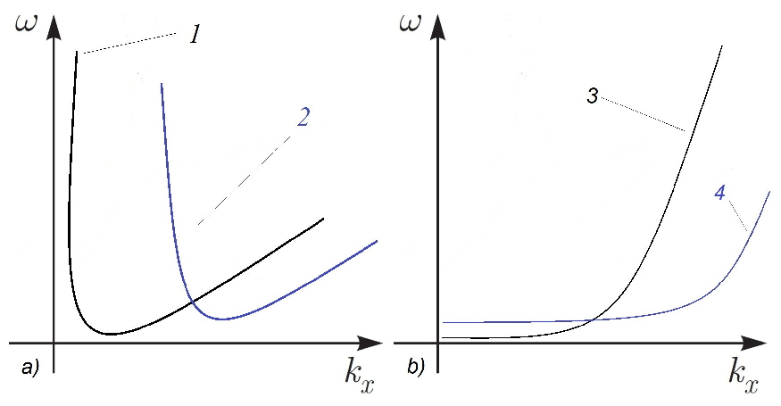
Both obtained dispersion relations of magneto-Rossby waves (in horizontal and in vertical magnetic fields) allow the existence of three waves satisfying phase matching condition (${\omega }_1\left({\mathbf{k}}_1\right)+{\omega }_1\left({\mathbf{k}}_2\right)={\omega }_1\left({\mathbf{k}}_3\right)$ and ${\mathbf{k}}_1+{\mathbf{k}}_2={\mathbf{k}}_3$). It is shown in Figure 2a for magneto-Rossby waves in an external vertical magnetic field, and in Figure 2b for magneto-Rossby waves in a horizontal magnetic field [34].

By means of a multiscale asymptotic method we have obtained amplitude equations for magneto-Rossby waves in a two-layer shallow water model in analogous form with equations in Section 2. These equations describe parametric instabilities in both cases of an external vertical magnetic field and a horizontal field [34]. Since the equations of three-wave interactions for a stratified fluid in the two-layer approximation differ only in the interaction coefficients, the same parametric instabilities that were found in Section 2 are realized in the two-layer model. The main difference in our case is in the increments of parametric instabilities and threshold values, which now depend on the ratio of densities.

It should be noted that the two-layer MHD shallow water equations are two-dimensional and do not allow for vertical changes in the parameters of the system. For a more accurate study of wave processes in a continuously and stably stratified plasma layer, we use a three-dimensional MHD system in the Boussinesq approximation. The results can be found in [56].

4. Zonal Flows in Two-Dimensional Magnetohydrodynamic Turbulence on a Beta Plane

Below, the MHD description of the rotating plasma is used to study 2D MHD turbulence and zonal flows origination in incompressible approximation [21]. The evolution of the vorticity $\omega$ and magnetic potential A of a two-dimensional MHD flow of a viscous fluid (plasma) with density $\rho ={\rho }_0=const$ in the $\beta$-plane approximation is described by equations:

$$\frac{\partial \omega }{\partial t}=J(\psi ,\omega )+\beta \frac{\partial \psi }{\partial x}+\frac{1}{4\pi \rho }J(A,\Delta A)+\nu \Delta \omega ,$$

(22)

$$\frac{\partial A}{\partial t}=J(\psi ,A)+\eta \Delta A,$$

(23)

where $\psi$ is the stream function, $\omega =-{\nabla }^2\psi$, $J(a,b)=\frac{\partial a}{\partial x}\frac{\partial b}{\partial y}-\frac{\partial a}{\partial y}\frac{\partial b}{\partial x}$ is the Jacobian of $a(x,y)$ and $b(x,y)$, $\nu$ is the kinematic viscosity, and $\eta$ is magnetic diffusion coefficient. The vorticity and stream function are related to the two-dimensional velocity field $(u_x,u_y)$ as:

$$\omega =\frac{\partial u_y}{\partial x}-\frac{\partial u_x}{\partial y};u_x=\frac{\partial \psi }{\partial y};u_y=-\frac{\partial \psi }{\partial x}.$$

(24)

The magnetic potential is related to the two-dimensional magnetic field $(B_x,B_y)$:

$$B_x=\frac{\partial A}{\partial y};B_y=-\frac{\partial A}{\partial x}.$$

(25)

Thus, we can reconstruct two-dimensional velocity field and two-dimensional magnetic field using Equations (24) and (25).

In the $\beta$-plane approximation Coriolis parameter f depends on the latitude to describe spherical effects in the Cartesian system of coordinates in Equation (8). The local two-dimensional ($2\pi \times 2\pi$) region on the sphere with periodic boundary conditions is considered. The x axis is directed along the azimuth and the y axis is opposite to the latitude (colatitude).

The first results of numerical simulations of 2D MHD Equations (22) and (23) with a spatial resolution of $1024\times 1024$ with different Rossby parameters $\beta$ are outlined [21]. Numerical experiments were performed for magnetohydrodynamics with equal initial kinetic and magnetic energy ($E_V^0=E_M^0=E_0$, where $E_V^0$ and $E_M^0$ are the initial kinetic energy and magnetic energy, respectively). Initial energies are set by the parameter $E_0$ that was chosen such that the Reynolds and magnetic Reynolds numbers were $Re=Rm\simeq {10}^5$. Correspondingly, the magnetic Prandtl number of the studied flows is $P{r}_m=\nu /\eta =1$. The initial conditions are set in the central ring of Fourier harmonics with radius $k_0=20$ which is outside the dissipative region. The Rossby parameters $\beta$ are such that the Rhines scale given by equation $k_{\beta }=\sqrt{\beta /2U}$, where U is the rms velocity of the turbulent flow, did not exceed $k_0$ (initial Fourier harmonics lie in the turbulence dominant region). All numerical experiments were performed up to the time $T=500$ expressed in dimensionless quantities, which can also be written as $T\simeq 17.8·T_0$, where $T_0=2\pi /U$ is the eddy turnover time in the turbulent flow at the initial time. We performed the experiments up to the time $T=500$ which is much longer than the time for system to adapt to the initial conditions ($T\gg T_0$) and is much less than the time of complete dissipation ($T\ll T_{dis}$). 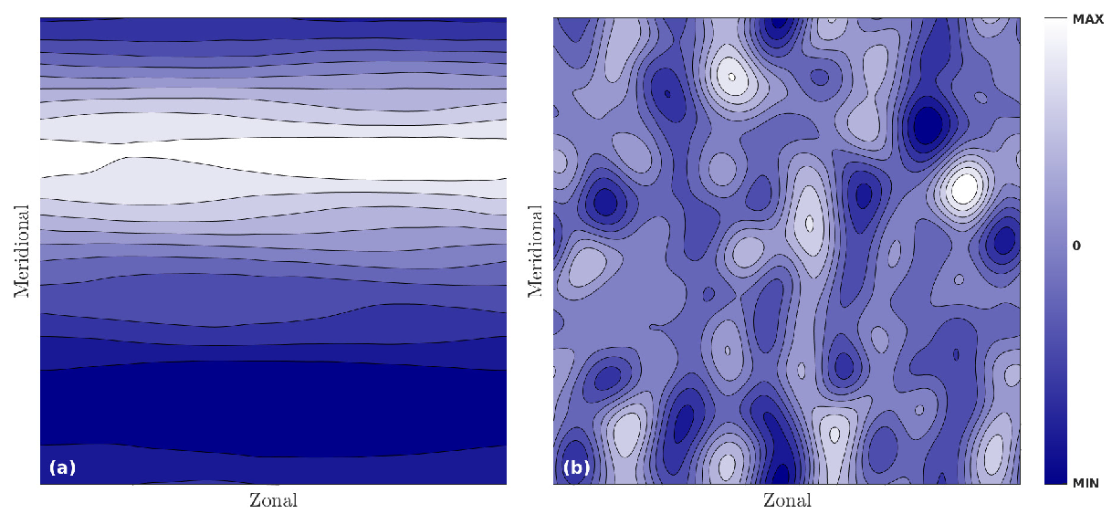To analyze the results of the numerical simulation, the contour lines of the stream function and magnetic field are considered. Figure 3 shows contour lines of the stream function and magnetic field on the (latitude, longitude) plane at $T=500$. White and blue regions correspond to the maximum and minimum values of the stream function respectively.

In the case of two-dimensional decaying MHD turbulence on the $\beta$-plane ($\beta =25$), the calculations show that zonal flows are formed after multiple merging of small eddies into large ones owing to the inverse energy cascade if the initial kinetic and magnetic energies are equal to each other. The coexistence of regularly positive (white) and negative (blue) regions along longitude in Figure 3a indicates that the velocity of flows in these regions is directed in one direction (along and against longitude, respectively). Such regions along or against longitude limited in latitude are called zonal flows. The shift of zonal flows along the longitude is due to the appearance of isotropic magnetic islands (closed magnetic field lines). Thus, contour lines of the stream function have bends associated with the magnetic field configuration. Figure 3b shows the computed contour lines of the magnetic field. The configuration of the magnetic field has meridional anisotropy: There are field lines elongated along the entire meridional direction. Field lines are perpendicular to zonal flows because of the freezing of the magnetic field. The performed numerical experiments demonstrate the formation of magnetic islands (closed field lines in Figure 3b) in the process of transition to a quasistationary state.

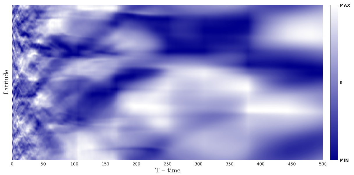
The time dependence of zonal flows in the case of MHD turbulence ($\beta =10$) is also analyzed. Figure 4 shows the time dependence of the zonally averaged field of the zonal velocity $V_x\left(y\right)$ for the case of MHD turbulence. The color in this figure varies from white corresponding to the maximum value of the function $V_x\left(y\right)$ to blue corresponding to the minimum value.

If the initial kinetic and magnetic energies are equal to each other and the Rossby parameter is $\beta =10$ zonal flows have a complex time dynamics: White and blue regions in Figure 4 are shifted along the longitude or are merged into wider regions. The performed calculations [21] show that the shift of zonal flows along the longitude is due to the appearance of isotropic magnetic islands (closed magnetic field lines) in the system. A similar situation is observed for the cases of MHD turbulence with the Rossby parameters $\beta =25;50$, in spite of strong anisotropy demonstrated in [21].

For the completeness of the physical picture, we present the results of the simulation of $\beta$-plane MHD turbulence spectra in the context of comparison of two-dimensional MHD turbulence and neutral fluid turbulence on the $\beta$-plane. We compared spectra of the kinetic energy for the case of the neutral fluid and the total energy for the case of MHD turbulence at the Rossby parameter $\beta =10$. 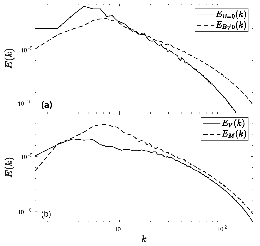Figure 5 shows spectra at the time $T=56\simeq 2T_0$ where the energy has already been redistributed from the initial state to the entire spectrum. Further analysis of spectra evolution is given in [57]. The time T is much smaller than the time of dissipation of the system $T\ll T_{dis}$.

Figure 5a shows the wavenumber distributions of kinetic (solid line) energy $E_{B=0}\left(k\right)$ in the neutral case and the total (dashed line) energy $E_{B\ne 0}\left(k\right)=E_V+E_M$ in the case of MHD turbulence for $\beta =10$. Figure 5b shows the wavenumber distributions of kinetic (solid line) energy $E_V\left(k\right)$ and magnetic (dashed line) energy $E_M\left(k\right)$ in the case of MHD turbulence for $\beta =10$.

According to Figure 5a, the wavenumber range consists of two regions: (i) The region of low wavenumbers where the energy spectra increase with k and (ii) the region of high wavenumbers where the energy spectra decrease with increasing k. The kinetic energy in the region of low wavenumbers in the neutral case is higher than the total energy in the case of MHD turbulence. The maximum of the kinetic energy spectrum in the neutral case is observed at $k=4.5$ in agreement with the theoretical Rhines scale $k_{\beta }=4.7$. The energy is concentrated at the boundary between wave and turbulent dynamics, the inverse energy cascade terminates at the Rhines scale and zonal flows are formed. The maximum of the total energy spectrum in the case of MHD turbulence is observed at $k=6.5$ and is due to the formation of magnetic islands in the system. In the region of high wavenumbers, the total energy in the case of MHD turbulence decreases more slowly than the kinetic energy in neutral fluid turbulence, similar to the case without rotation [20].

Furthermore, we compared the spectra of the kinetic and magnetic energies for the case of MHD turbulence at the Rossby parameter $\beta =10$. It is seen in Figure 5b that the magnetic energy is much higher than the kinetic energy. At equal initial kinetic and magnetic energies, the adaptation of the system to the initial conditions occurs at the beginning of the experiment: The kinetic energy is transformed to the magnetic energy and the ratio of the energies is established at the value $E^M/E^V\simeq 1.5$ as in the case without rotation [20]. The maximum of the kinetic energy spectrum in the case of MHD turbulence is observed at $k=3.5$ in agreement with the theoretical scale estimate $k_{\beta }^M=3.7$ obtained in [21]. As a result, the region of wave vectors of zonal flows for decaying MHD turbulence is smaller than that for neutral turbulence. Our calculations confirm that the proposed scale specifies the lower bound of the inertial interval of turbulence at which the inverse energy cascade terminates. The detailed study of spectra of two-dimensional MHD turbulence on the $\beta$-plane is outlined in [57].

5. Conclusions

A number of new applications in astrophysics and recent space observations have actualized the problem of study and description of rotating plasma behavior. Here, we briefly reviewed recent achievements in studies of large-scale magnetohydrodynamic flows in plasma astrophysics. We focused on magnetohydrodynamic shallow water approximation for rotating plasma and on two-dimensional magnetohydrodynamic flows on a beta-plane.

The MHD shallow-water equations in the presence of rotation with an external magnetic field were revised by supplementing them with equations derived from the magnetic field divergence-free condition. New system revealed the existence of the third component of magnetic field in this approximation and provided its relation with the horizontal magnetic field. The presence of a vertical magnetic field significantly changed the dynamics of wave processes in astrophysical plasma compared to the neutral fluid and plasma layer in a horizontal magnetic field. Moreover, we considered effects of stratification in two-layer MHD shallow water model with rotation and external magnetic field, dividing a thin layer of plasma into two layers with different densities. The new system was reduced to the obtained one-layer MHD shallow water system in an external field by equating the heights and densities of the layers. Through the use of the developed two-layer model, we derived modifications for magneto-Rossby waves, related to stratification.

The shallow-water approximation (one-layer and two-layer models) have been used for the development of the weakly nonlinear theory of magneto-Rossby waves both in external vertical magnetic field and in the absence of magnetic field, as well as for stationary states with the presence of a horizontal field (poloidal, toroidal, and their sum). A qualitative analysis of the dispersion curves for the Rossby waves in magnetohydrodynamics revealed the possibility of three-wave interactions in the weak nonlinearity approximation. The weakly nonlinear theory of magneto-Rossby waves developed using the method of multiscale asymptotic expansions and three-wave equations for slowly varying amplitudes were briefly outlined. An approximate analysis of the resultant systems of equations revealed that two types of parametric instability could evolve in the system: Parametric decay and parametric amplification of magneto-Rossby waves.

The first results of the numerical simulation of two-dimensional decaying MHD turbulence on the $\beta$-plane were discussed. Numerical simulations demonstrated the formation of zonal flows in MHD turbulence on the $\beta$-plane. Zonal flows in MHD turbulence on the $\beta$-plane significantly differed from flows in the neutral fluid. Zonal flows in MHD turbulence were unsteady because of the presence of isotropic magnetic islands in the system. The inverse energy cascade in decaying MHD turbulence on the $\beta$-plane terminated at the scale that differed from the Rhines scale but was consistent with our new criterion of the boundary between wave dynamics and MHD turbulence.