1. Introduction
The understanding of wave dynamics in the nearshore is still challenging because of the high variability of the nearshore wave process in both the surf and swash zones. Thus, investigation of nearshore wave phenomena is necessary in itself, as well as essential to describe wave-induced coastal disasters such as flooding, coastal erosion, and fragility of coastal structures.
Remote sensing is considered the most appropriate approach to describe nearshore waves taking into account the difficulties of obtaining sufficient data that are continuous and quality controlled in space and time in the conventional way [
1].
A few studies have been published on tracking individual waves across a cross-shore transect of interest in coastal video imagery on the surf and swash zone of natural beaches. Yoo et al. [
2] used filter-based image processing methods, in particular Radon transformation [
3], to track individual waves on time-space images, the called timestacks images, which do not contain the full variability of wave parameters in the surf zone.
Vousdoukas et al. [
4] introduced wave run-up measurements based on timestack images generated from coastal video imagery by extracting and processing time series of the cross-shore position of the swash extrema. The estimated wave run-up height was more accurate than those from available empirical formulations, but in their procedures manual supervision is required to accurately extract the run-up height from the timestack images.
More recently, Stringari et al. [
5] tacked waves in the surf zone using learning-based computer vision techniques to detect breaking waves accurately. Breaking waves are derived from coastal video imagery by identify the white foam and tracking accumulating timestack images in a cross-shore direction. It detects white pixel intensity peaks generated by breaking waves, confirms these peaks as true wave breaking events by learning from the data’s true color representation, clusters individual waves and derives the optimal wave paths. Thus, it can be applied directly to any timestack image without additional complex image transformation required as in Yoo et al. [
2]. However, the method still requires that timestack images are made for each specific cross-shore orientation and a manually implemented training dataset of timestack images with labels identify breaking waves, sand, and undisturbed water.
In this paper, we propose a new approach of observing the behavior of waves in the surf and swash zone from coastal video imagery, which is a fully automated method of applying deep neural networks to track individual transformed and propagated waves in space and time. It allows a full characterization of the wave breakers including the wave run-up, with an unsupervised learning approach, which tracks coastal waves from wave crest until they break and disappear in swash zone.
2. Methodology
Waves in the surf zone are traced by applying deep neural networks to coastal video imagery taken at Anmok beach in Korea. The proposed wave-tracking framework consists of three parts: image enhancement by preprocessing raw video images for learning, scene separation to consider only the wave motion in the video and wave-tracking through unsupervised image registration. We next describe the considered training and validation dataset and then these three procedures separately with experiments.
2.1. Unlabeled Video Dataset
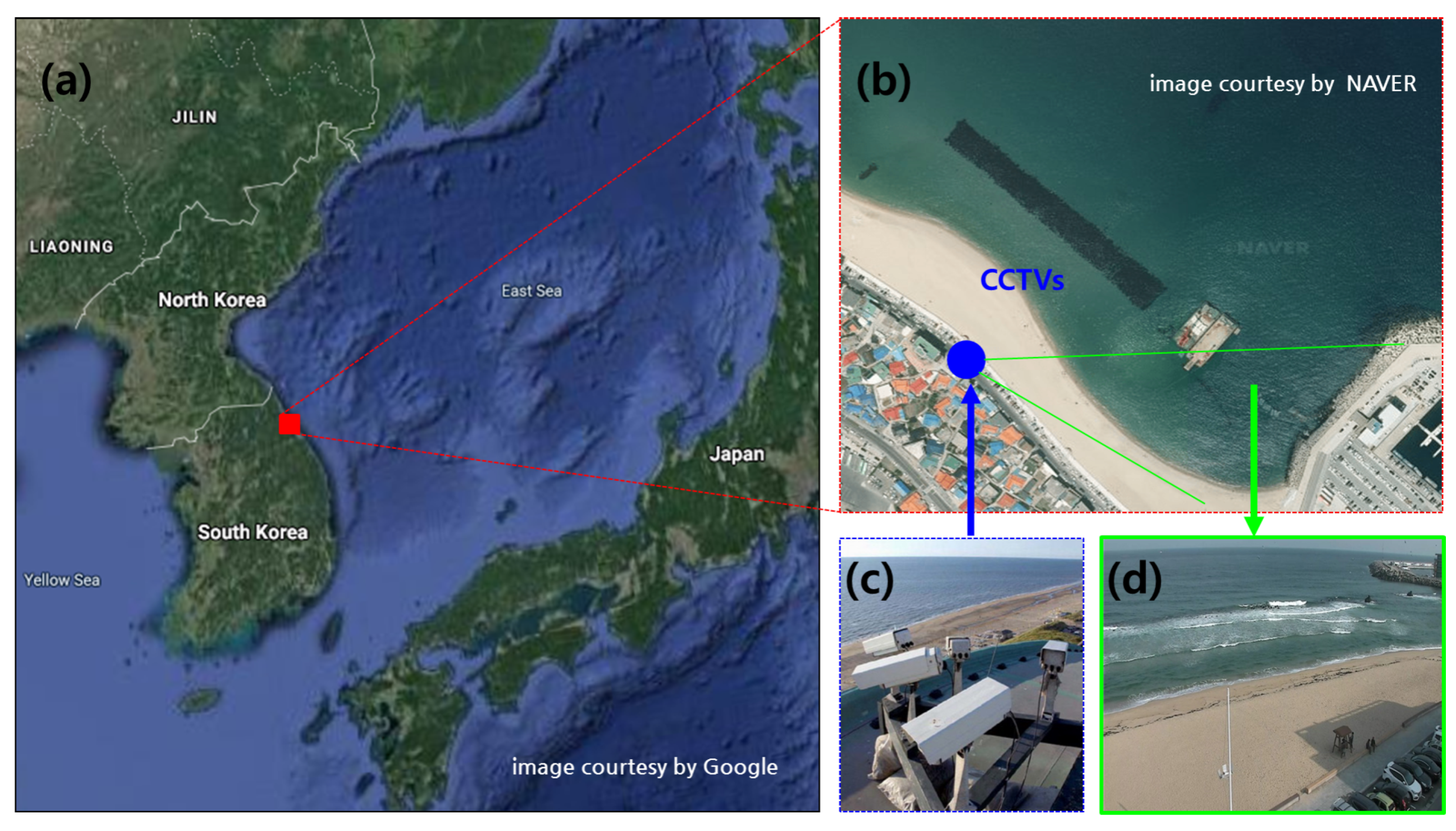
The study area, Anmok beach, is a straight almost 4 km long micro-tidal wave dominated environment located on the east coast of South Korea (
Figure 1a,b). The wave climate during winter is dominated by swells coming from the north-northeast, some of them severe and attacking the coastline. The observed current magnitudes are generally low (in the order of 0.1~0.2 m/s). Most of the time the significant wave height is low (Hs < 1.5 m) and the peak wave period is below 7.5 s. However, the coast is occasionally hit by severe storms with maximum offshore significant wave height higher than 9 m [
6].
In the last few decades, the east coast of South Korea has been suffering from erosion. To understand the associated physical process, a video monitoring system using general CCTVs (Closed Circuit Television) has been installed and video data has been stored since 2016 (
Figure 1c,d).
The field of view covers a span of about 150 m in both the along-shore and cross-shore directions. The spatial and temporal resolution of the video is and 30 frames per second (FPS). For training and validation of the proposed networks, we randomly selected 233 and 360 video clips in November 2016 and 2017, respectively at an 8:2 ratio. All videos are recorded in daytime and cover different wave breaking and light conditions and each video clip has about 10 min long. For the unsupervised learning without any labeling task, all frames of the videos recorded at 30 FPS are used without downsampling.
2.2. Video Enhancement
Computer vision is an interdisciplinary scientific field that deals with how computers can be used to gain high-level understanding from digital images or videos. Deep learning has enabled the field of computer vision to advance rapidly in the last few years.
Despite the advances in optical cameras, the captured image or recorded video often still come with visual degradation due to the environmental conditions such as bad weather, low light and underwater as well as features of optical system itself such system noise, optical distortion, motion blur, downsampling and compression loss. Due to these issues comprehensive methods that improve the perceptual quality of images or video are in high demand.
In recent years, deep image/video enhancement methods have demonstrated their superiority for derain, dehazing, denoising, deblurring as well as super-resolution. Most of those problems can be posed as translating an input image into a corresponding output image. In analogy to automatic language translation, we define automatic image-to-image translation as the task of translating one possible representation of a scene into another, given a large amount of training data.
The Pix2Pix architecture proposed by Isola et al. [
7] is widely used as the baseline structure for image-to-image translation. Pix2Pix uses a generative adversarial network (GAN) [
8] to learn a function to map from an input image to an output image. The network is made up of two main pieces, the generator, and the discriminator. The generator transforms the input image to get the output image. The discriminator measures the similarity of the input image with an unknown image (either a target image from the dataset or an output image from the generator) and tries to guess whether it has been produced by the generator.
The video of winter coastal hazardous regions is distorted by bad weather conditions such as rainy weather, wind and fog. It is, therefore, essential to improve the quality of video imagery before processing it further. In particular, image distortion caused by raindrops is a major problem in applying visual intelligence for image-based wave-tracking. To remove raindrops and to restore background information in coastal video imagery, a Pix2Pix network is implemented using a paired set of raindrop and clear images. The network has a structure of a GAN with a generator and a discriminator, which are trained simultaneously to transform distorted images by raindrop to clear images.
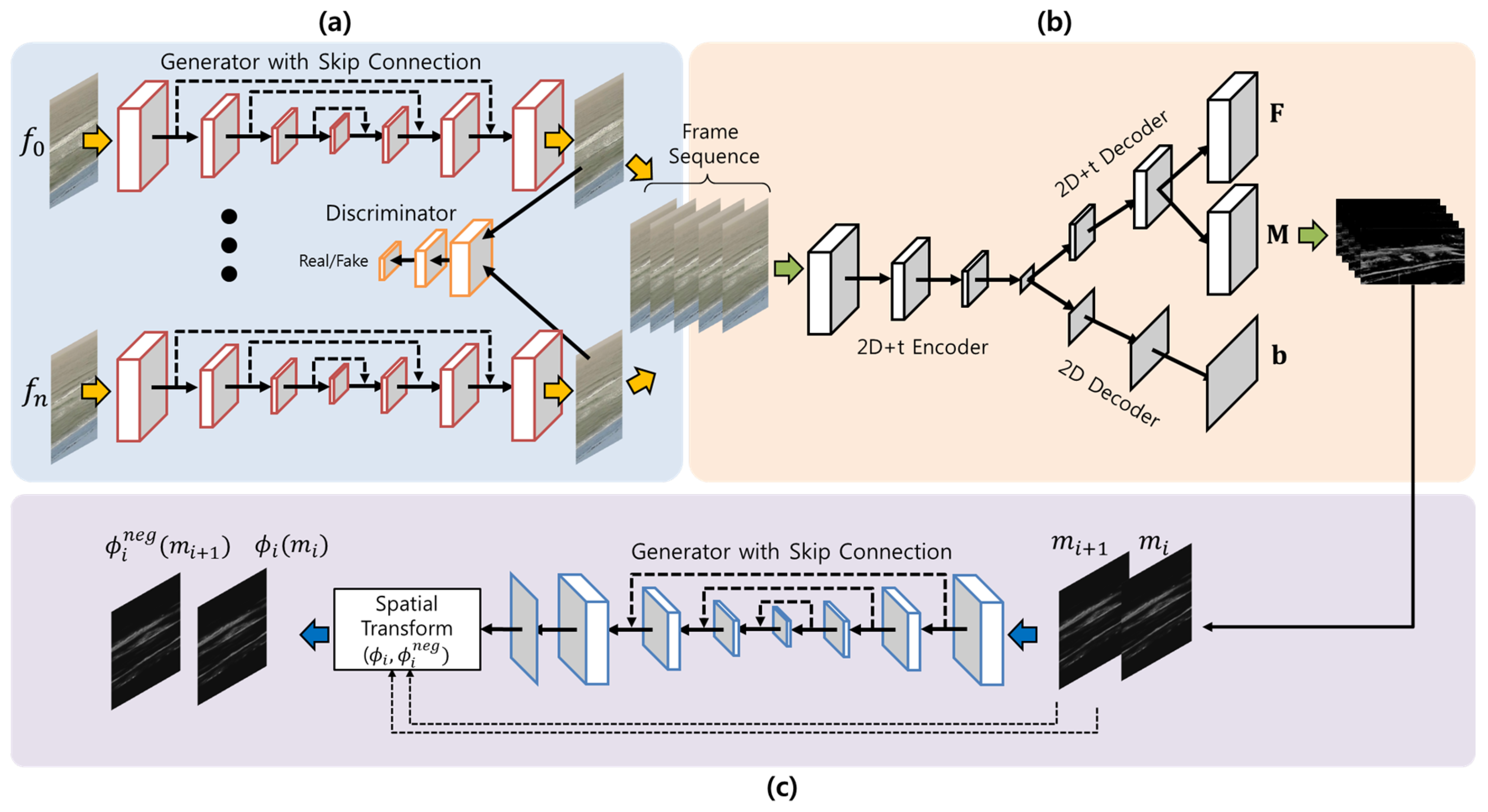
The architecture of the Pix2Pix is shown in
Figure 2a. The network consists of the generator (
G) that generates a target image (
y) from the input image (
x), and a discriminator (
D) that discriminates between the generated image and the target image.
x is input into the generator as the image impeded by raindrops, and the generator uses this input to generate an image
where the raindrops are removed. The generator creates
as close as possible to the corresponding target image
y without raindrop distortion and it also learns parameters to generate
more realistic to fool the discriminator which has a role to discriminate between
and
y. Through this repetitive learning process, the generator and discriminator simultaneously are trained in an adversarial manner.
For the Pix2Pix network pre-training, we use an open dataset including paired images with and without raindrops in the land environment collected by Qian et al. [
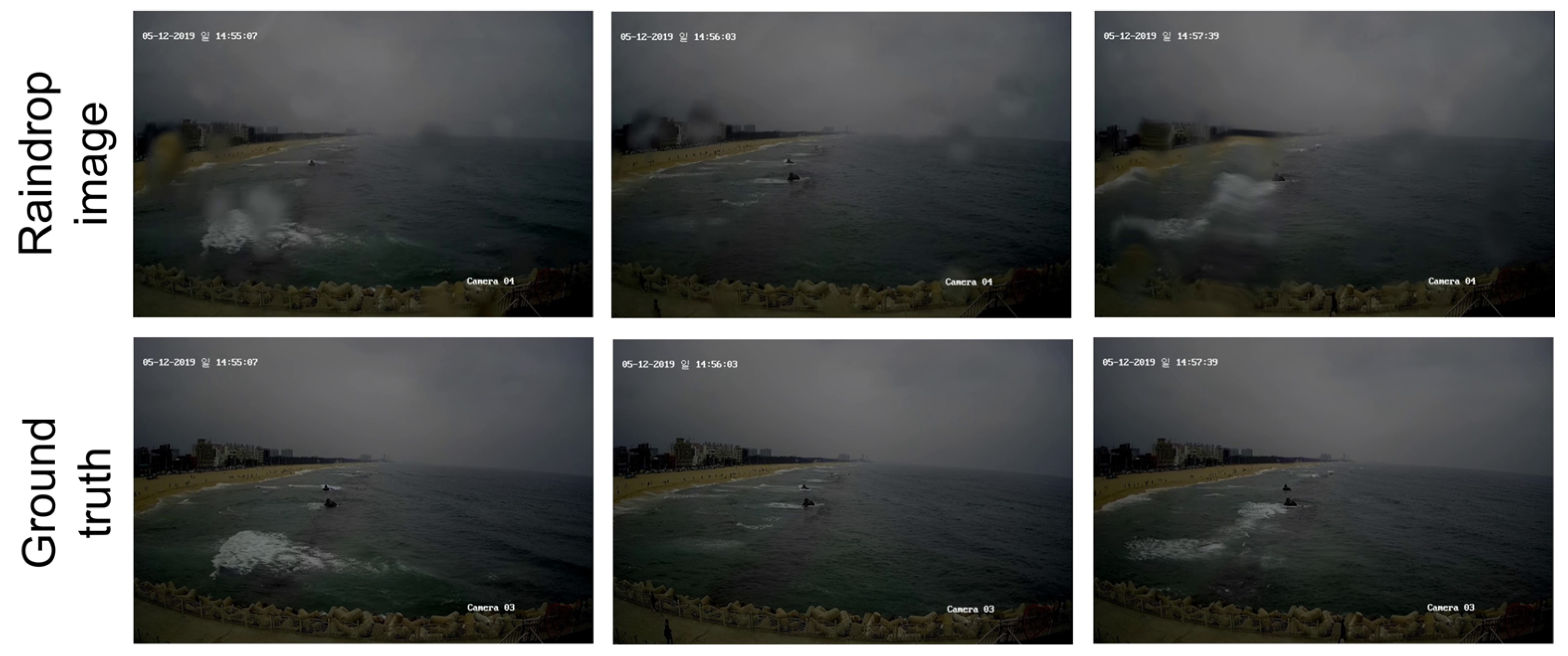
9]. After the pre-training, we train the pre-trained model using a dataset paired with and without raindrops, which was acquired directly using two CCTVs installed side by side in Anmok beach [
10]. 17,002 paired images are extracted from the 10 min. long video clips. 12 video clips classified with raindrop patterns were used to fine-tune the transferred pre-trained Pix2Pix network parameters of which some samples are shown in the
Figure 3.
2.3. Hydrodynamic Scene Separation
Understanding object motions and scene dynamics is also a key issue in computer vision for both video recognition for behavior classification and video generation for future prediction. It is a challenging problem to learn how scenes transform with time from large amounts of unlabeled video, because there are a vast number of ways that objects and scenes can change.
Vondrick et al. [
11] proposed a generative adversarial network for video with a spatio-temporal convolutional architecture that untangles the scene’s foreground from the background to capture some of the temporal knowledge contained in large amounts of unlabeled video. They introduced a two-stream generative model that explicitly models the foreground separately from the background, which allows enforcing that the background is stationary, helping the network to learn which objects move and which do not. The proposed concept is applied to separating wave motion from ambient information in coastal video images.
Before tracking the coastal waves, a deep autoencoder network is established to extract the hydrodynamic scene only, by minimizing the ambient light effect in the coastal video imagery. The proposed model extends to an autoencoder which compresses and reconstructs the input video images by removing the discriminator from the GAN structure and creating natural video images by separating the foreground and background [
12].
The proposed network shown in the
Figure 2b generates a background image (
b), which is common across time, and foreground images (
F), which represents temporal changes along time, in the process of compressing and reconstructing sequential video frames. In addition, the pixel-wise weights of all image sequences are determined in the process of restoring the original input video imagery by combining the background image and the foreground image sequences. The maps of the pixel-wise weights are called mask images (
M) and contain the wave motion information along time.
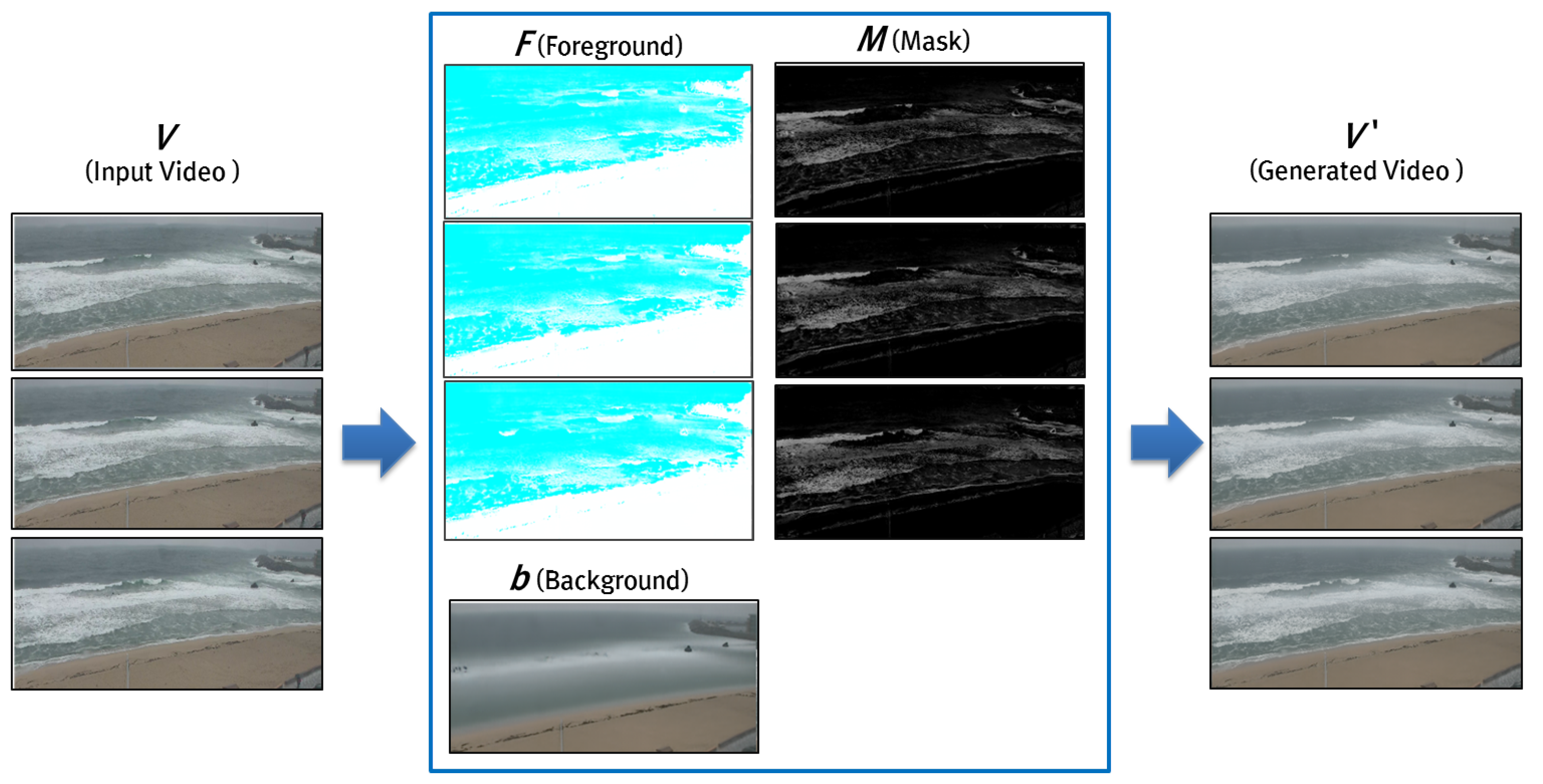
As depicted in
Figure 4, considering the input video imagery as
V (
), a generated video
can be expressed as follows by combining separated foreground image sequences (
) and a common background image (
b) with mask images (
):
The separated background images contain solely the environmental factors, such as the ambient light affecting the overall frame of the input video. In the mask sequences, spatio-temporal changes between frames is expressed as real numbers in the range of 0 and 1. Furthermore, the solely the wave propagation captured in the input video, is kept in the mask sequences.
2.4. Unsupervised Image Registration
Image registration is typically formulated as an optimization problem to seek a spatial transformation that establishes pixel/voxel correspondence between a pair of fixed and moving images by maximizing a surrogate measure of the spatial correspondence between images, such as structural similarity or image intensity correlation between registered images.
In particular, deep learning techniques have been used to build prediction models of spatial transformations for achieving image registration. The models are designed to predict spatial relationships between image pixel/voxel from a pair of images, to learn informative image features and a mapping between the learned image features and spatial transformations that register images in a training dataset.
In medical image analysis, non-rigid inter-modality image registration is a core problem for many clinical applications, as is allows for the use of the complementary multimodal information provided by different imaging protocols. Balakrishnan et al. [
13] presented a learning-based framework for deformable, pairwise medical image registration. It formulates registration as a function that maps an input image pair to a deformation field that align these images. We adopt this framework for coastal wave-tracking.
In the third and final procedure, the propagating waves are tracked by registering consecutive images in the separated mask sequences (
M) using a spatial transformer network to find nonlinear spatial transformation between them. As shown in
Figure 2c, by inputting two consecutive frames (
), the spatial displacement map representing nonlinear spatial transformation from the current mask frame (
) to the next frame (
) is generated. The displacement map includes the displacement vector information from the pixels of the
to the corresponding pixels of the
.
The spatial transformation network comprises the U-net [
14] to generate affine transformation parameters to convert each pixel of the two consecutive frames to the related pixel location. This neural network also constructs the inverse transformation map, in which each displacement vector of the constructed transformation map is inverted, and by learning to adjust
and
to each other, it realizes the diffeomorphic registration allowing the inverse operation of the transformation map.
The L2-norm loss function (
) for training the spatial transformer network in Equation (
2) is used to derive optimal spatial transformation map (
) registering consecutive two input images by maximizing similarity between images and minimizing abnormal image deformation.
is the differential value of transformation vector. The diffusion minimizing loss term performs a regularization function that minimizes sudden changes in the displacement vectors. is the inverse map of the displacement map . The network computes the similarity measure after changing each consecutive frame (, ) using and for the diffeomorphic coordination.
2.5. Experiments
The training dataset used for training the proposed model, as shown in
Figure 2, consisted of 17 days of video taken in October 2016. From the video, 5,610,407 frames were extracted corresponding to 187,013 seconds of daytime images from 9 a.m. to 6 p.m. 20 % of them were used as a validation dataset for optimization. For successful unsupervised learning, the temporal resolution of the original video, which is 30 FPS, was kept. However, considering the available computer resources and computation time, the spatial resolution has been reduced from
to
. In particular the scene separation network is a very memory-intensive task because it needs to look at the whole data during the learning process to separate a mask for the common background and the moving foreground in successive frames from the training dataset.
The Adam optimizer [
15] was used for training the model and the learning rate was set to 0.0001. The server used in this experiment has an Intel
i7 3.5 GHz, 128 GB memory CPU, and NVidia (Intel, Santa Clara, CA, USA)
Titan XP GPU with 12 GB video memory (Nvidia, Santa Clara, CA, USA). It took approximately one and a half days to training the model.
In the scene separation network, the mean square error between the input image and the reconstructed image was measured for the validation dataset, and early stopping [
16] is used to stop learning in the section where the error increases to prevent overfitting. In addition, considering the memory-intensive task of model training, the batch size was set to 1, and group normalization [
17] was used instead of batch normalization.
For the image registration, the optimal epoch was determined by measuring the structural similarity and mean squared error between the registered image at time t and the target image at time t + 1 for the validation dataset, with a batch size of 5.
3. Results
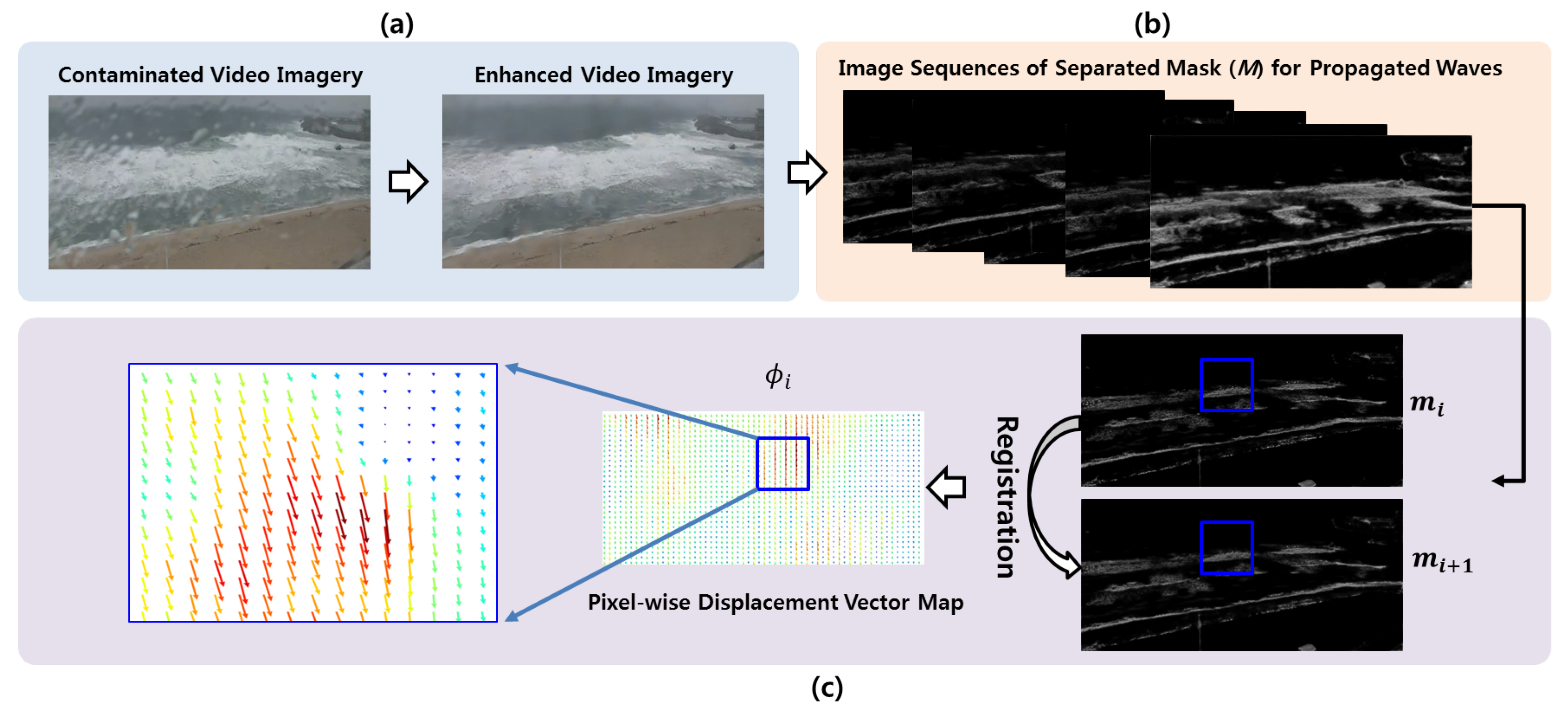
Figure 5 shows the proposed wave-tracking process by visualizing the results of the deep neural networks from Anmok beach video images. In
Figure 5c, the displacement vectors between two corresponding pixels in
and
are represented using arrows.
The input video imagery passes through the first network for video enhancement, as shown in
Figure 2a for better image quality. For instance, if the input image is contaminated by raindrops, the raindrops are removed and the wave information in the background is restored as shown in
Figure 5a. The enhanced video imagery is then used as the input data of the hydrodynamic scene separation network as shown in
Figure 2b, to separate the wave movement information from the environmental information such as light effects. When the input image sequence passes through the network, it is separated into the foreground, background, and mask. The mask
M includes only the wave movement information, as shown in
Figure 5b, and is then used as input to the registration network for wave-tracking, as shown in
Figure 2c. The vector field shown in the left part of
Figure 5c is a displacement map of the nonlinear spatial deformation vector, computed pixel-wise from the register of two consecutive images.
The hyper-parameters of the networks were determined by assessing images similarity between and (). () is the result of applying the nonlinear spatial deformation matrix to . It is considered that the higher structural similarity of two images, for example and (), the better the tracking of the propagated waves. To avoid overfitting, we choose a model in epoch with the lowest mean square error and standard deviation as well as high structural similarity during the model validation process. It means that the correspondence between the transformed image (()) and the target image () is the highest after image registration, and the displacement vector field () represents the movement of waves with high accuracy. The structural similarity is 0.983 and the mean squared error is 0.147. The index of structural similarity is calculated by obtaining the correlation coefficient between two images in pixel-wise way, with a minimum value of 0 and a maximum value of 1.
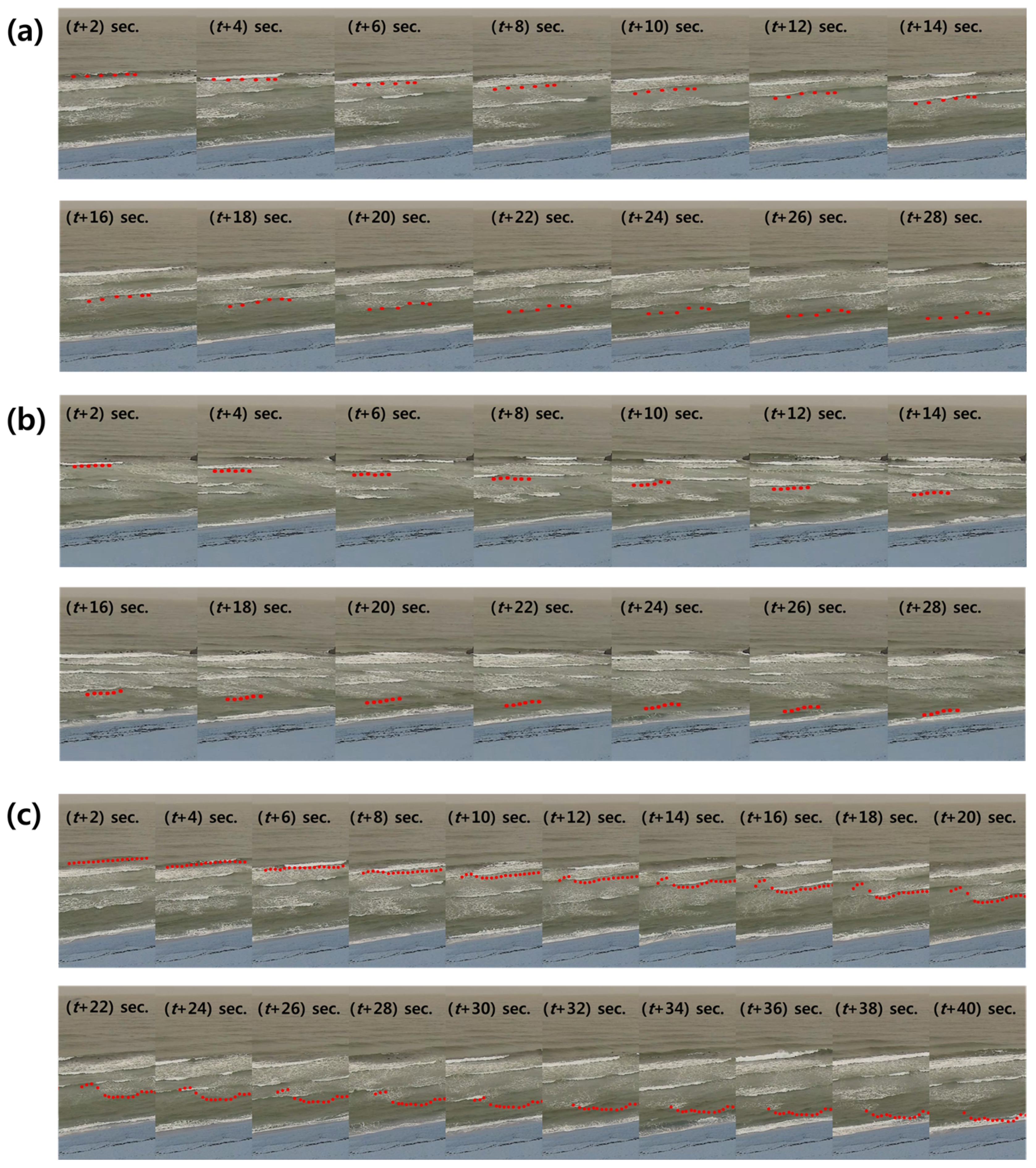
To ensure the performance of wave-tracking visually in space and time, randomly assigned multiple landmarks on the wave crest line in the video and tracking the movement of the landmarks as the wave propagates, breaks and disappears. To visualize the coastal wave-tracking from shoaling non-breaking to wave swash, 6 and 20 landmarks are assigned to the three test videos randomly along the wave crest line with circles filled with red color in 6 and 20 pixels, as shown in
Figure 6. The position of the landmarks is individually updated by adding the displacement vectors with the largest magnitude in the 3 × 3 neighbors around each landmark.
In
Figure 6a,b, the image registration algorithm visually confirms that the 6 landmarks on the wave crest are reasonably well tracked during 30 s. considering in total 900 frames. In
Figure 6c, it is also visualizing the wave-tracking performance using the 20 landmarks on the wave crest during 40 s. considering in total 1200 frames. If you look at the four landmarks on the left, you can see that the remaining 16 landmarks track well along the wave crest, while the tracking accuracy degrades for (
t + 8) s. ∼ (
t + 20) s. The reason is that as shown in
Figure 7, when registering successive images, the shape of wave crest in the input target image is not clear itself. Thus, the next position of the 4 landmarks to be tracked is determined by referring to the neighbor’s movement.
The tracking algorithm helps to track the wave crest more correctly against image noise and abnormal movement by using a model that learned the behavior of wave propagation from the training dataset and neighbor’s movement in test dataset. The landmarks are not merged, but they can overlap together depending on the tracking result.
To demonstrate the tracking of broken waves,
Figure 8 shows the tracking points of two sequential waves mapping with circles filled with red and green colors on the edge of white foam of breaking waves. We assigned 14 and 10 landmarks respectively at 10∼12 pixels intervals. The location of each landmark was updated by adding displacement vectors, which were estimated through the unsupervised image registration at each pixel, every 0.03 s. As shown in
Figure 8, the landmarks on the breaking foam of white pixel were tracking well the individual waves that broke and disappeared as they propagated over time. After the tracking, we confirmed that the landmarks were properly positioned at the edges of the white foam.
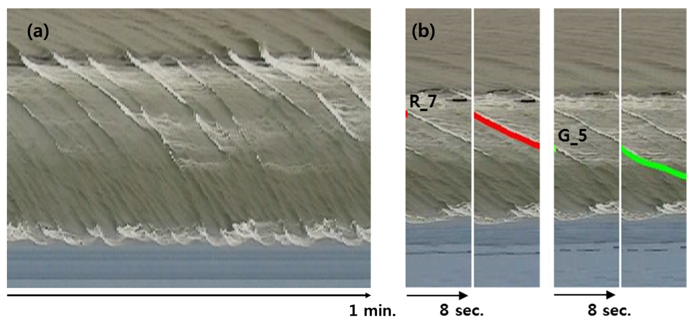
Figure 9a provides an illustration of timestack images, as used in conventional image processing approaches for the analyzes the coastal waves. The timestack images for one min. are produced from images in
Figure 8 along the transect connection R_7 and G_5 shown in the leftmost image in
Figure 8. The two landmarks of R_7 and G_5 in
Figure 8 were selected in the cross-shore transect, and the tracking results for the two landmarks during 8 s. are shown in
Figure 9b.
In
Figure 9a, a time series of wave trajectories including the incipient shoaling and breaking points with created turbulent whitewater spilling for breaking waves are clearly visible. Furthermore, in
Figure 9b, we can visually confirm that our tracking results agree well with the wave trajectories for the two landmarks.
The time series of velocity estimated by tracking at each landmark are shown in
Figure 10. The velocity at randomly selected 6 landmarks, shown in the leftmost image in
Figure 8, was calculated based on pixels of the image moving per 0.3 s. The pixels containing each landmark are at a distance of approximately 0.1 to 0.35 m. The velocity at each landmark on the edge of white foam of broken waves was estimated during 10.7 s. with 320 frames. The velocity was calculated from the real distance and time required for the pixels corresponding to each landmark. From
Figure 10b, it can be seen that the velocity decreased as the landmarks move approaching to the swash zone, i.e., as the white foams disappeared. Because when the broken waves reach the shore, they dissipate their energy in the form of wave swash.
From numerical experiments using CST3D-WA validated with in situ measurements, Kim et al. [
18] report that the instantaneous current speed was about 0.46 m/s in the onshore of Anmok beach in January 2015. In addition, Lim et al. [
19] conducted multiple Lagrangian GPS drifter experiments to measure the surface nearshore currents in Anmok beach for 2 hours in January 2016 and February 2018. They presented that the current speed on onshore of Anmok beach is about 0.25 and 0.38 m/s. Although the quantities presented in each study do not exactly match, as well as the measured times and methods all differ, they can be roughly regarded as in close range. For a quantitative evaluation and accurate comparisons, it is necessary to further examine and plan experimental and analysis methods.
4. Conclusions
In this work, we introduced deep neural network approach to tracking waves using coastal video imagery in the surf and swash zones. It contains not only wave-tracking but also video enhancement to improve the quality of images contaminated by raindrops and hydrodynamic scene separation to extract only the movement of waves excluding the effects of ambient light.
The proposed method consists of three parts: (1) video enhancement, (2) hydrodynamic scene separation and (3) wave-tracking. For video enhancement, a Pix2Pix network, trained using paired raindrop and clean videos, was applied to remove image distortions by raindrops and to restore background wave information. Next, a hydrodynamic scene of propagated wave information was separated from ambient information in the enhanced coastal video imagery using a deep autoencoder network. For coastal wave-tracking, propagating waves were tracked by registering consecutive images in the quality-enhanced and scene-separated coastal video images using a spatial transformer network.
The instantaneous wave speed of each individual wave crest and breaker in the video domain was estimated through learning the behavior of transformed and propagated waves in the surf zone. Unlike the conventional approach, the learning-based method takes time to training the model, but it has the advantages that it is possible to use a trained model in near real time for inference and prediction. It also allows longer time tracking than conventional methods, and simultaneously can track multiple groups of waves in an arbitrary region, rather than being limited to individual waves across a particular cross-shore transect in coastal video images. Moreover, the applicability of the proposed approach is high given that it uses unsupervised learning, which learns the behavior of breaking waves from large amounts of video images without labor-intensive labeling. Since annotating video is expensive and ambiguous, we believe learning from unlabeled data without supervision is a promising direction.
From the visualization of water tracking by placing multiple points along the wave crest line and breaking waves on the image sequence of propagated waves, the tracking results mostly matched well visually, but were somewhat inaccurate when the crest line were not clearly distinguished and the breaking waves were widely scattered or disappeared. To learn the wave movement robustly in surf and swash zone, it is necessary to use higher-resolution video images or a variety of videos acquired from other coasts. Because the higher spatio-temporal resolution of the video, the better we can examine the water evolution.
We have also been working on lab experiment and on the validation of the techniques presented in this article for hydrodynamics scene separation and unsupervised image registration-based coastal wave-tracking [
20]. These techniques were applied to wave flume videos and compared with the results of an acoustic Doppler velocimetry (ADV) measurement and of one conventional image processing technique of particle image velocity. The comparisons were done for the location where the ADV was installed and the estimated wave celerity by the proposed approach showed good agreement with the ADV measurement. However, to evaluate the performance of the applied techniques more accurately, more measurements from multiple points are required. In addition, for further verification of the proposed approach validation data should be obtained through field measurements despite the difficulties of collecting them.
In terms of computational effort, our proposed model under the experimental conditions described in Chapter 2 took one and a half days to train. However, the advantage of our proposed method and other machine learning approaches, is that once the model has finished the training, the input is analyzed immediately. Conversely, in conventional image processing approaches, the processing of each new image involves going through the whole process from image processing to analysis.
The proposed shore-based remote sensing with unsupervised deep learning framework has the potential to be used in novel investigations of understanding and modeling nearshore wave dynamics and surf and swash zone phenomena such as dune process for beach erosion and accretion that require wave-tracking. In particular, the propose method can be used to improve swash dynamics prediction through more accurate measurement of run-up height by characterizing breaking waves in the swash zone [
21].
For the future work, we will evaluate the inverted depth in shallow water and wave speed obtained through wave-tracking quantitatively by comparing with in situ measurement of depth and water elevation using multi-beam and pressure sensors in coastal wave domain and the network will be improve based on that comparison.
