Diurnal and Seasonal Variations of Surface Energy and CO₂ Fluxes over a Site in Western Tibetan Plateau

Abstract

Land surface process observations in the western Tibet Plateau (TP) are limited because of the abominable natural conditions. During the field campaign of the Third Tibetan Plateau Atmospheric Scientific Experiment (TIPEX III), continuous measurements on the four radiation fluxes (downward/upward short/long-wave radiations), three heat fluxes (turbulent sensible/latent heat fluxes and soil heat flux) and also CO₂ flux were collected from June 2015 through January 2017 at Shiquanhe (32.50° N, 80.08° E, 4279.3 m above sea level) in the western Tibetan Plateau. Diurnal and seasonal variation characteristics of these surface energy and CO₂ fluxes were presented and analyzed in this study. Results show that (1) diurnal variations of the seven energy fluxes were found with different magnitudes, (2) seasonal variations appeared for the seven energy fluxes with their maxima in summer and minima in winter, (3) diurnal and seasonal variations of respiration caused by the biological and chemical processes within the soil were found, and absorption (release) of CO₂ around 0.1 mg m⁻² s⁻¹ occurred at afternoon of summer (midnight of winter), but the absorption and release generally canceled out from a yearly perspective; and (4) the surface energy balance ratio went through both diurnal and seasonal cycles, and in summer months the slopes of the fitting curve were above 0.6, but in winter months they were around 0.5. Comparing the results of the Shiquanhe site with the central and eastern TP sites, it was found that (1) they all generally had similar seasonal and diurnal variations of the fluxes, (2) caused by the low rainfall quantity, latent heat flux at Shiquanhe (daily daytime mean always less than 90 W m⁻²) was distinctively smaller than at the central and eastern TP sites during the wet season (generally larger than 100 W m⁻²), and (3) affected by various factors, the residual energy was comparatively larger at Shiquanhe, which led to a small surface energy balance ratio.

1. Introduction

The Tibetan Plateau (TP) is the most prominent and complicated terrain on the globe. It stretches about 1000 km along latitude and 2500 km along longitude, and its average elevation exceeds 4000 m above mean sea level. Researchers have shown that the TP is one of the key areas affecting extreme weather and climate events all over the globe [1,2,3,4,5,6,7,8,9,10,11,12,13,14]. The land–atmosphere interaction of the Tibetan Plateau is important for the formation and development of the Asian monsoon system [15,16,17,18,19,20,21,22,23,24]. Especially, the thermal effects through surface heat fluxes to the atmosphere over the TP greatly influence the atmosphere circulations both regionally and globally [11,16,25].

Over the past decades, to understand the land–atmosphere interaction over the TP, intensive experiments and studies were carried out to investigate the observed turbulent fluxes over the TP. By using the data from the Global Energy and Water Cycle Experiment (GEWEX) Asian Monsoon Experiment (GAME) in 1998, Tanaka et al. [26] identified a seasonal-scale variation in the surface energy closure ratio at the Amdo planetary boundary layer site in the eastern TP, while Choi et al. [27] compared the fluxes obtained by flux variance and eddy covariance methods over a short grass prairie near Nagqu site in the northern TP. Through the observation during the Coordinated Enhanced Observing Period (CEOP) Asian–Australia Monsoon Project (CAMP) in the TP (CAMP/Tibet, 2001–2005) [28], Ma and Ma [29], Yao et al. [30] and Guo et al. [31] examined the energy exchange over different sites in the central and northern TP. Yang et al. [32] gathered data from the previously mentioned experiments and analyzed the characteristics of the downward shortwave and longwave radiations over 11 stations from the eastern to western TP. Gu et al. [24] collected surface fluxes data at two sites continuously in 2008 in the central TP and studied their surface energy budget. Based on two-year measurements over two contrasting landscapes (bare land and natural alpine meadow) at Wudaoliang (34.82° N, 92.92° E, a northeastern TP site), You et al. [33] presented and analyzed local energy budget and phenology.

From the above-mentioned studies, characteristics of surface energy partitioning were identified both diurnally and seasonally mostly over the central, eastern and northern TP, that were relatively easy to access. However, long-term observation of surface fluxes in the western TP was not available until the start of the Third Tibetan Plateau Atmospheric Scientific Experiment (TIPEX III) in July 2014 [13], which included turbulent fluxes observation at a western TP site Shiquanhe. Xin et al. [34] used the data collected at the Shiquanhe site in July–September 2014 to explore the surface energy balance and the associated uncertainties. It was found that as a heterogeneous site, the sensible and latent heat fluxes consisted of only 65% of the available energy at the Shiquanhe site. With TIPEX III continuing, long term data now become available at this site, which provides a chance to understand the diurnal and seasonal variations of the turbulent fluxes there. This study examines the characteristics of radiation fluxes, turbulent heat fluxes, and CO₂ flux by using the consecutive observations from June 2015 to January 2017. The rest of this paper is organized as follows. Descriptions of the site, measurements, and methods are given in Section 2. Section 3 provides results, including the meteorological background, diurnal and seasonal variations of radiation and turbulent fluxes, and analysis of energy balance closure. Summary and discussions are found in Section 4.

2. Materials and Methods

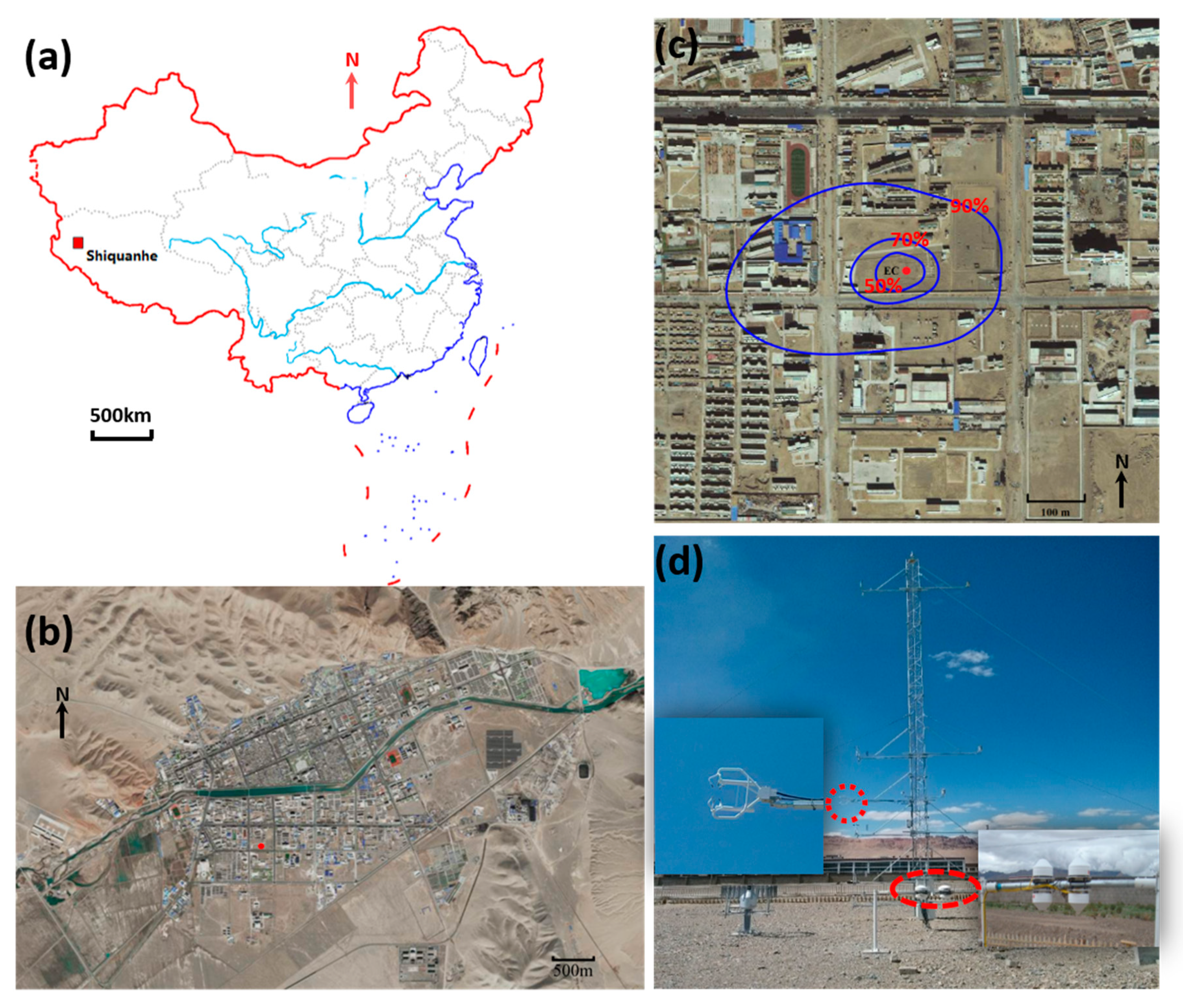
2.1. Site

The observation period in this study was from 9 June 2015 to 31 January 2017. To ensure the power supply, the site was set in Shiquanhe town in the western TP (32.50° N, 80.08° E, 4279.3 m above sea level). North of Shiquanhe Town lies the Kailash Range, while the west and south sides are surrounded by the Himalayas. The site is located in the transition zone between the monsoon region and the non-monsoon region, and it is affected by the India monsoon to some extent. The climate of the site is categorized into mid-latitude arid continental temperate climate. Figure 1 shows the site location, underlying surface condition, footprint, and instruments. The underlying surface consists of sand and a small amount of gravels. Under near-neutral conditions, the dynamic roughness length z_0m can be calculated using Monin–Obukhov similarity theory with the equation: $z_{0\mathrm{m}}=\left(z-d)/\exp (\frac{uk}{u_{*}}\right)$, where friction velocity $u_{*}$ and mean wind speed u are measured by the three-dimensional ultrasonic anemometer, z is the observation height, d is the zero-plane displacement height, and k is the von Karman constant (0.4). Here, we only have one level observation, so that the displacement height cannot be calculated. The surface roughness is different at different azimuth due to the heterogeneity of the site. At south and east, it is generally open and flat, and the displacement height can be neglected, and the surface roughness has a value of around 0.01 m. However, at west and north, there are buildings and $z_{0\mathrm{m}}+d/\exp (\frac{uk}{u_{*}})$ has a value of around 0.3 m.

To estimate both the source area and the relative contribution of each surface elements to the measured fluxes, the footprint analysis is conducted by using the Kljun et al. model [35]:

$$\phi \left(\gamma \right)={{\displaystyle \int }}_R{Q}_{\phi }\left(r+r^{\prime }\right)f\left(r,r^{\prime }\right)\mathrm{d}{r}^{\prime }$$

(1)

where $\phi$ is the measured flux value at r, $Q_{\phi }$ is the source emission rate at r + r’, R is the domain of integration, f is the transfer function (footprint function), and it can be expressed in terms of a crosswind-integrated footprint and a crosswind dispersion function. A detailed description of the model can be found in Kljun et al. [35]. The footprint contour lines of 50%, 70%, and 90% are shown in Figure 1c. It can be found that 90% of the measured fluxes come from within 300 m of the observation tower, and the surface is relatively flat within 70% of the source area. However, there are some buildings and roads located in 90% of the source area.

2.2. Micrometeorological Measurements

2.2.1. Fast Response Measurements

The eddy covariance instruments were installed at 5.45 m (sensors’ center height) above the ground surface (Figure 1d), and they consisted of a three-dimensional ultrasonic anemometer, a gas analyzer, and a controller. The three-dimensional ultrasonic anemometer (CSAT3A, Campbell Scientific Inc., USA) was used to measure wind components (i.e., u, v, and w) and sonic virtual air temperature. The separated, in situ, open-path, mid-infrared absorption gas analyzer (EC150, Campbell Scientific Inc., Logan, UT, USA) was used to simultaneously measure the absolute density of carbon dioxide and water vapor. A controller (EC100, Campbell Scientific Inc., Logan, UT, USA) was used to control the gas analyzer and sonic anemometer, and synchronously sample data from them. The controller was also used to control a temperature thermistor probe and a barometer to measure the ambient air temperature and barometric pressure, respectively. All signals of the sensors were recorded at a sampling rate of 10 Hz and averaged over 30-min periods by a data-logger (CR3000, Campbell Scientific Inc., Logan, UT, USA). These sensors were calibrated before installation. Quality control and turbulent flux calculation were carried out with EddyPro 6. 2.1 (LI-COR Inc., Lincoln, USA, 2017) for the eddy covariance data. The processing steps and flux corrections are listed as follows: (1) Remove the spikes of the raw time series with a criterion of $\left(\overline{X}-4\sigma \right)<x\left(t\right)<\left( \overline{X}+4\sigma \right)$, where x(t) denotes the measurement (i.e., horizontal wind speed u and v, vertical wind speed w, etc.), $\overline{X}$ is the mean over the data block and σ is the standard deviation [36], (2) skip the turbulent data block missing more than 10%, (3) use double rotation method for the sonic anemometer tilt correction [37], (4) use 30-min as the flux averaging interval to compute turbulent fluxes, (5) use the WPL (Webb, Pearman, and Leuning) method for density corrections [38], (6) use high/low-frequency spectral corrections to compensate for flux losses [39], (7) remove the flux data in rainy (snowy) or fog conditions as eddy-covariance systems do not work properly under such environment.

2.2.2. Slow Response Measurements

Other supporting data, such as radiation, air temperature, air pressure, relative humidity, soil moisture, soil temperature, and soil heat flux, were collected synchronously during the experiment. Upward/downward shortwave/longwave radiation components were measured with two pyranometers (CMP22, Kipp & Zonen B.V., Delft, The Netherlands) and two pyrgeometers (CGR4, Kipp & Zonen B.V., Delft, The Netherlands) mounted at the height of 1.5 m. Soil heat flux at a depth of 0.05 m was measured by a heat flux plate (HFP01SC, Hukseflux Thermal Sensors B.V., Delft, The Netherlands), while soil temperature and volumetric water content at five depths (0.05, 0.1, 0.2, 0.4, and 0.80 m) were measured by a thermocouple (109, Campbell Scientific Inc., Logan, UT, USA) and a water content reflectometer (CS 616, Campbell Scientific Inc., Logan, UT, USA), respectively. The ground surface temperature was measured by an infrared radiometer (IRR-P, Apogee Inc., Austin, USA) mounted at the height of 1.5 m AGL. A tipping bucket rain gauge (TE525M, Texas Electronics Inc., Dallas, TX, USA) mounted at the height of 70 cm was used to measure precipitation. All the data were sampled each minute, averaged (Precipitation was accumulated.) every 30 min, and recorded with a CF card by a data-logger (CR3000, Campbell Scientific Inc., Logan, UT, USA).

2.3. Methods

The surface energy balance over the Gobi canopy can be approximated by:

$${Rn=H+LE+G}_0+Re,$$

(2)

where Rn is the net radiation (W m⁻²), H and LE are the sensible and latent heat fluxes (W m⁻²), G₀ is the soil heat flux at the ground surface (W m⁻²), Re (W m⁻²) is the residual energy (W m⁻²). Rn can be approximated with the four components of radiation fluxes:

$$Rn=DSR+DLR-USR-ULR,$$

(3)

where DSR is the downward shortwave radiation (W m⁻²), DLR is the downward longwave radiation (W m⁻²), USR is the upward shortwave radiation (W m⁻²), and ULR is the upward longwave radiation (W m⁻²).

Turbulent sensible and latent heat fluxes are calculated as:

$$H=\rho C_p\overline{w^{\prime }{T}^{\prime }},$$

(4)

$$LE=L\rho \overline{w^{\prime }{q}^{\prime }},$$

(5)

where $\rho$, C_p, and L are the density of air (kg m⁻³), the specific heat of air (J kg⁻¹ K⁻¹), and the latent heat of vaporization (J kg⁻¹), respectively. w’, T’, and q’ are the fluctuations in the vertical wind component (m s⁻¹), air temperature (K) and specific humidity (g Kg⁻¹), respectively. Relevant calculation methods can be found in [40,41].

The soil heat flux at the surface, G₀, is estimated with:

$$G_0=G_{0.05}+C_g∆z\partial T/\partial t,$$

(6)

where G_0.05 is the soil heat flux measured at depth of 0.05 m with a heat flow plate, C_g is the volumetric heat capacity of the soil (J m⁻³ K⁻¹), which can be derived from soil components [42], ∆z is the thickness of the soil layer above the plate (i.e., 0.05 m) and T is the mean soil temperature of the layer, ∂T/∂t is the change rate of mean soil temperature. Here, T = (T₀ + T_0.05)/2, where T₀ is the ground surface temperature, and T_0.05 is the soil temperature measured at the depth of 0.05 m. Neglecting the heat contribution of air in the soil, the volumetric heat capacity is estimated by [43]:

$$C_g=\left(1-{\eta }_s\right)C_s+\eta C_w ,$$

(7)

where $\eta$ is the volumetric moisture content of soil and ${\eta }_s$ is the saturation value of sand soil moisture (0.395 m³ m⁻³) ([43], its Table A9), C_s is the volumetric heat capacity of dry sand soil (1.280 × 106 J m⁻³ K⁻¹) ([43], its Table A7), and C_w is the volumetric heat capacity for water (4.186 × 106 J m⁻³ K⁻¹).

The residual energy Re, also called absolute energy balance residual (AEBR) [44], is defined as the following formula:

$${Re=Rn-H-LE-G}_0.$$

(8)

It involves various processes, such as soil respiration, heat storage in soil and canopy [45,46], and phase change of water in the soil [47,48,49].

To assess the surface energy balance closure, two criteria are often used: Re (AEBR) and the surface energy balance ratio (SEBR) [50]. SEBR, marked as ε, also known as the surface heating rate, is defined as the ratio of the turbulent heat fluxes (H + LE) to the available energy fluxes (Rn − G₀) [51]. Ideally, when the surface energy balance (i.e., partitioning of Rn into LE, H, and G₀) is perfectly closed, ε should be equal to one. To obtain SEBR, one method is to derive linear regression coefficients from the least square relationship between (H + LE) and (Rn − G₀), and the slope is taken as the SEBR. The other method is to calculate the ratio between the cumulative sums of (H + LE) and (Rn - G₀) for a specific period [51,52,53], as follows:

$$SEBR=\frac{\sum \left(H+LE\right)}{\sum \left({Rn-G}_0\right)}$$

(9)

CO₂ flux is calculated using the following equation [54,55]:

$$F_{C{O}_2}=\overline{w\text{′}c\text{′}},$$

(10)

where $F_{C{O}_2}$ is CO₂ flux (mg m⁻² s⁻¹) and c’ is the fluctuation in the CO₂ concentration (mg m⁻³) [56].

3. Results

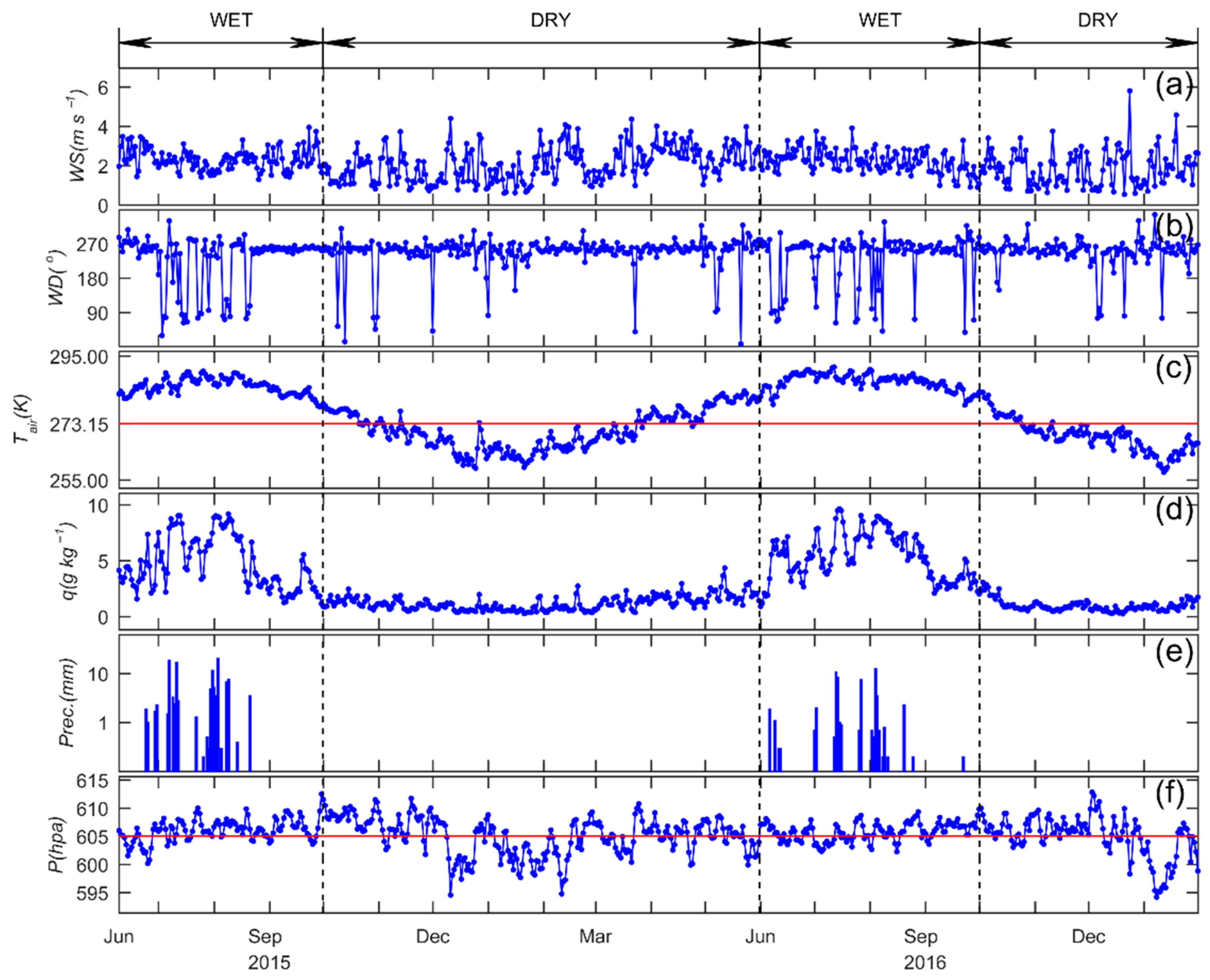
3.1. The Meteorological Background

The variations of the daily mean wind speed (WS in m s⁻¹), air temperature (T_air in K), specific humidity (q in g kg⁻¹), air pressure (P in hPa), and daily accumulated precipitation (Prec. in mm) from June 2015 to January 2017 are shown in Figure 2. Generally, all the meteorological elements had obvious seasonal cycles. June to September is categorized as wet season in this study due to the relatively high specific humidity and frequent precipitation events, while October to May is defined as dry season.

At this site, the wind speed was relatively low with its daily mean mostly below 3 m s⁻¹ for the whole year, and the maximum daily mean wind speed in this observation period was 5.8 m s⁻¹, but the maximum hourly mean wind speed reached 8.9 m s⁻¹. South-westerlies were dominant at this site and showed little season variation. However, the seasonal variation of air temperature was significant. The mean air temperature of the entire experiment was 276.6 K. In 2016, the annual mean air temperature was 276.5 K, the highest (lowest) monthly mean air temperature was 288.3 K (263.5 K) appearing in August (January). During the experiment period, daily mean air temperature reached a maximum of 291.3 K in July 2016, and a minimum of 257.5 K in January 2017, while the maximum 30-min air temperature of 298.1 K occurred at 19:30, 12 July 2016, and the minimum 30-min air temperature (251.0 K) occurred at 9:00, 25 December 2015.

The specific humidity was relatively low, and the mean specific humidity of the entire experiment was 2.6 g kg⁻¹. The difference in specific humidity between wet and dry season was obvious. In the year 2016, the average of specific humidity in the wet season was 5.3 g kg⁻¹, and in the dry season, it was 1.2 g kg⁻¹. In response to the precipitation, the 30-min specific humidity reached 12 g kg⁻¹ in the wet season (not shown) but kept less than 2 g kg⁻¹ in the dry season.

Almost all precipitation occurred in June–September in both 2015 and 2016. The total precipitation amounts from June to September were 119.9 and 58.9 mm in 2015 and 2016, respectively. The annual maximum daily precipitation of 20.4 mm occurred on 4 August 2015, and 12.8 mm occurred on 5 August 2016.

The 30-min air pressure ranged from 612.8 to 594.1 hPa with an average of 605.0 hPa in the observation period. Different from the plain area, the atmospheric pressure at Shiquanhe in the warm summer (June, July, and August) was slightly higher than in the cold winter (December, January, and February), exhibiting the typical alpine air pressure characteristics. In winter, some strong low-pressure center moved over this place and decreased the daily mean air pressure to 595.0 hPa.

3.2. Diurnal Variations

3.2.1. Radiation Components

To investigate the diurnal variations of the radiation components, the monthly averaged diurnal variations of the four radiation components (DSR, USR, DLR, and ULR) and the net radiation (Rn) are given in Figure 3. Intense diurnal variations were found in all the four radiation components. Because of the larger (smaller) solar altitude, larger (smaller) diurnal variations for DSR, USR and ULR showed in summer (winter) with magnitudes of 1078.24, 206.06, and 218.88 W m⁻² (632.14, 142.75, and 132.67 W m⁻²) in June (December) of 2016, but such a characteristic did not show in DLR, which was probably caused by the small values (around 150~320 W m⁻²) and weak diurnal fluctuations of DLR (about 50 W m⁻²). In the year 2016, the monthly averaged daily maximum DSR, USR, DLR, and ULR showed maximum (minimum) values of 1078.24, 206.06, 321.57, and 564.0 W m⁻² (632.15, 142.76, 196.25, and 363.33 W m⁻²) in the Jun, Jun, August, and Jun (December, January, January, and January), respectively. The monthly variation phase of DLR was one to two months behind the other radiation components, because of the slow response of the temperature of the upper atmosphere to the solar altitude change.

Rn was calculated with Equation (2) by using the four radiation components (i.e., DSR, USR, DLR, and ULR). Generally, Rn was mainly affected by DSR since it was the largest of the four radiation components and also the driving force of the other three. Here, Rn varied roughly from -130 at night to 600 W m⁻² at noon, heated the surface in the daytime while imposed a cooling effect on the surface after sunset. Similar results can also be found in the observations from Lhasa and several other stations in the central, Nyingchi and Litang in the Eastern TP, and Haibei in the northwestern TP [57,58,59]. In the year 2016, the yearly averaged Rn was 64.70 W m⁻², and the largest (smallest) monthly averaged daily maximum of Rn was 589.81 W m⁻² (311.64 W m⁻²) at noon in June (December), while the largest (smallest) monthly averaged daily minimum of Rn was −95.99 W m⁻² (−134.70 W m⁻²) at midnight in January (September).

The surface albedo was calculated as the ratio of USR to DSR. Affected by the diurnal variation of solar altitude, the surface albedo was also found changing diurnally between roughly 0.2 and 0.4, with the maximum in the morning and minimum at noon. Besides, caused by the seasonal variation of the soil water content, the surface albedo was slightly smaller in the wet season than in the dry season. In the year 2016, the averaged surface albedo was 0.21 in the wet season and was 0.25 in the dry season.

3.2.2. Heat and CO₂ Fluxes

Figure 4 shows the monthly averaged diurnal variation of turbulent sensible heat flux (H), turbulent latent heat flux (LE), soil surface heat flux (G₀), and CO₂ flux ($F_{C{O}_2}$) during this observation period. H, LE, and $F_{C{O}_2}$ were measured by fast response instruments and calculated using Equations (3), (4), and (5).

The diurnal variation of sensible heat flux was similar to that of Rn, with large positive values in the daytime but near zero or negative in the nighttime. The magnitude of the diurnal variation was larger in summer (maximum of 233.13 W m⁻² showed in May 2016) and smaller in winter (minimum of 104.59 W m⁻² showed in December 2016). In the year 2016, the yearly averaged sensible heat flux was 44.37 W m⁻², and the largest (smallest) monthly averaged daily maximum was 229.93 W m⁻² (87.00 W m⁻²) in May (December), while the largest (smallest) monthly averaged daily minimum was −2.91 W m⁻² (−17.60 W m⁻²) in August (December).

The diurnal variation of latent heat flux was small during the dry season and at night values within 5 W m⁻² were generally found, which could be attributed to the following factors: (1) Soil water was frozen when temperature was below zero, (2) soil water content was low and little water for evaporation at the surface, (3) little vegetation and then little water transpiration. The inter-month variation of latent heat was obvious. During the wet season, (1) the soil was thawed, (2) precipitation happened (as shown in Figure 2), and (3) large net radiation was presented, then the latent heat flux could be relatively large, and the diurnal variation became evident and reached a value of 42.2 W m⁻² at noon in August 2015.

Consistent with the sensible heat flux, soil surface heat fluxes (G₀) also had a significant diurnal variation with the diurnal maximum values (about 140~240 W m⁻²) at noon and diurnal minimum values (about −50~−100 W m⁻²) at midnight during the observation period. The positive (negative) values at noon (night) indicated downward (upward) transportation of heat flux to deeper soil (surface). The maximum (minimum) magnitude of the diurnal variation of G₀ occurred in July 2015 (January 2017) and the associated daytime peak value reached 235.6 (139.0) W m⁻².

CO₂ is one of the most important greenhouse gases and attracts attention globally. Wohlfahrt [60], Xie [61], and Mamtimin Ali [62] found that desert could behave as carbon sink, because: (1) The abiotic process and air-soil CO₂ concentration gradients in surface boundary layer caused such desert carbon uptake [62], (2) alkaline soil on land absorbed CO₂ with an inorganic, non-biological process [61], (3) a small amount of precipitation could activate bio-autotrophic respiration in the soil and heterogeneous respiration of soil organisms, resulting in enhanced autotrophic respiration and abnormal breathing of soil organisms in the surface moist layer. Here, measurements of $F_{C{O}_2}$ were also carried out in the observation period. Figure 4d showed that $F_{C{O}_2}$ was generally positive in autumn (September, October, and November) and winter but showed relatively significant negative values in spring (March, April, and May) and summer. Large absorption (release) of CO₂ occurred in the afternoon of summer (midnight of winter) and the monthly mean daily maximum absorption (release) was around 0.1 mg m⁻² s⁻¹ in Jun (December) 2016. From a yearly perspective, these positive and negative values generally canceled out, and the yearly average of $F_{C{O}_2}$ in 2016 was close to zero. In this period, the diurnal variation in late autumn or early winter and late spring or early summer was generally more significant compared to the other periods, while the largest (smallest) monthly averaged daily maximum of $F_{C{O}_2}$ was 0.12 mg m⁻² s⁻¹ in October 2016 (0.02 mg m⁻² s⁻¹ in July 2015), and the largest (smallest) monthly averaged daily minimum of $F_{C{O}_2}$ was 0.00 mg m⁻² s⁻¹ in December 2015 (−0.12 mg m⁻² s⁻¹ in May 2016).

3.3. Seasonal Variations

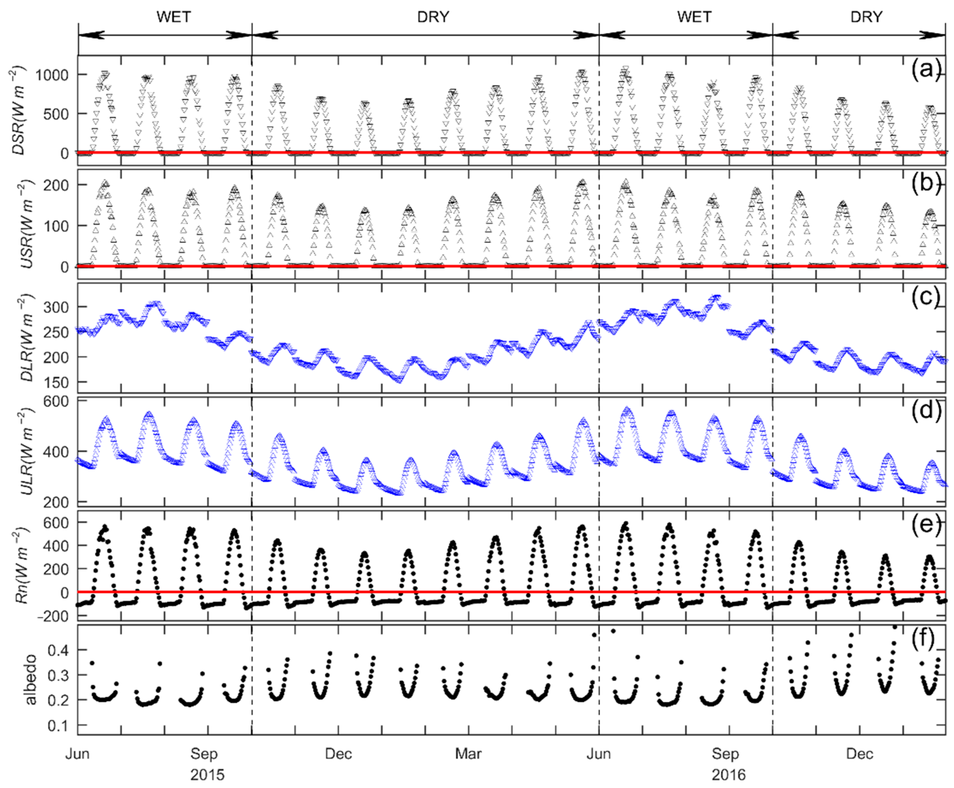
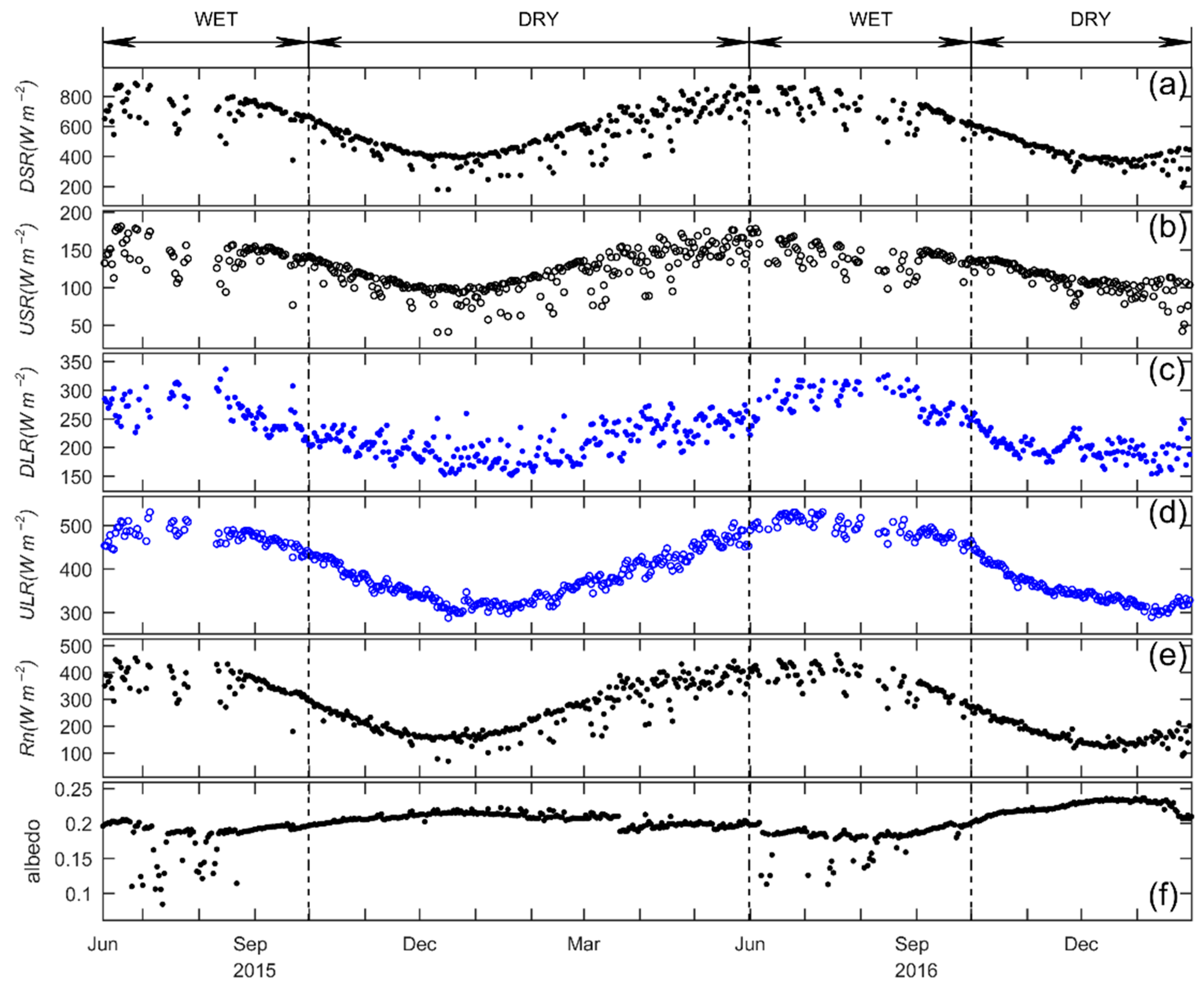
3.3.1. Radiation Components

Figure 5 shows the daily daytime (10:00–19:00 local time) means of the four radiation components (DSR, USR, DLR, and ULR), net radiation, and albedo. All the four radiation components exhibited significant seasonal variation due to the seasonal variation of solar altitude, and DSR, USR, and DLR showed some scatters caused by clouds. DSR, USR, and ULR generally shared the same phase of seasonal variation and had their maxima (minima) in June (December) with values of 885.52 W m⁻², 181.15 W m⁻² and 530.65 W m⁻² (178.39 W m⁻², 40.42 W m⁻², and 286.95 W m⁻²), respectively. However, the seasonal variation phase of DLR was behind those of DSR and USR for about one to two months, respectively. DLR showed maximum (minimum) in August (January) with values of 336.53 W m⁻² (151.34 W m⁻²). Caused by the lag of DLR seasonal variation, seasonal variation of daily mean Rn was also slightly behind the phase of DSR and USR, with its maximum (minimum) value of 465.41 W m⁻² (68.79 W m⁻²) shown in July (December). The surface was bare and had little vegetation all year round so that the seasonal variation of albedo was relatively invariant, and for most of the observation period, it fluctuated around 0.20 ± 0.03. Some scattered dots lower than 0.17 in the wet season were caused by the precipitation event. Skipping these scattered dots, the slightly higher albedo was shown around December than around July, which was caused by the drier (moister) soil in the winter (summer) season.

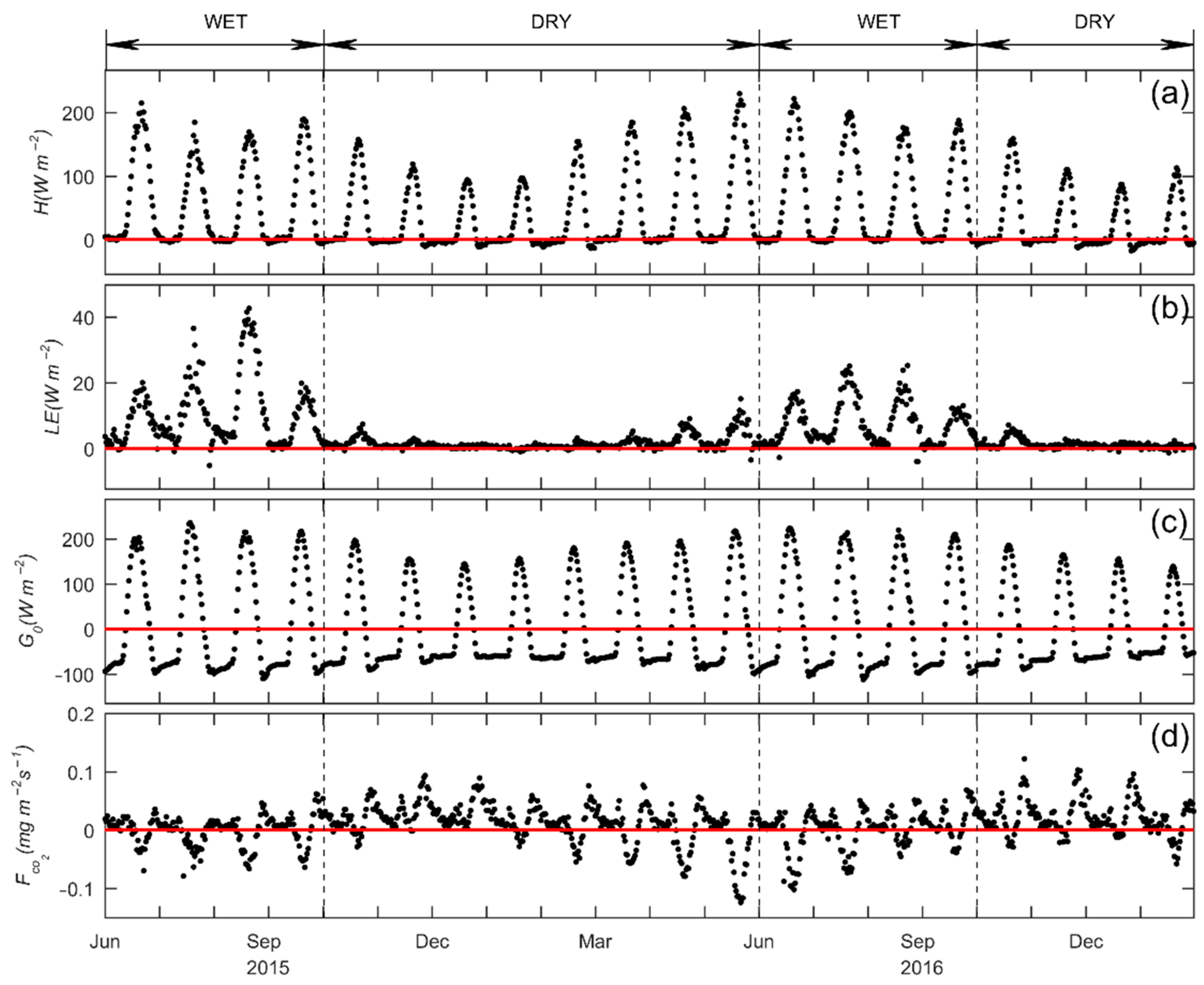
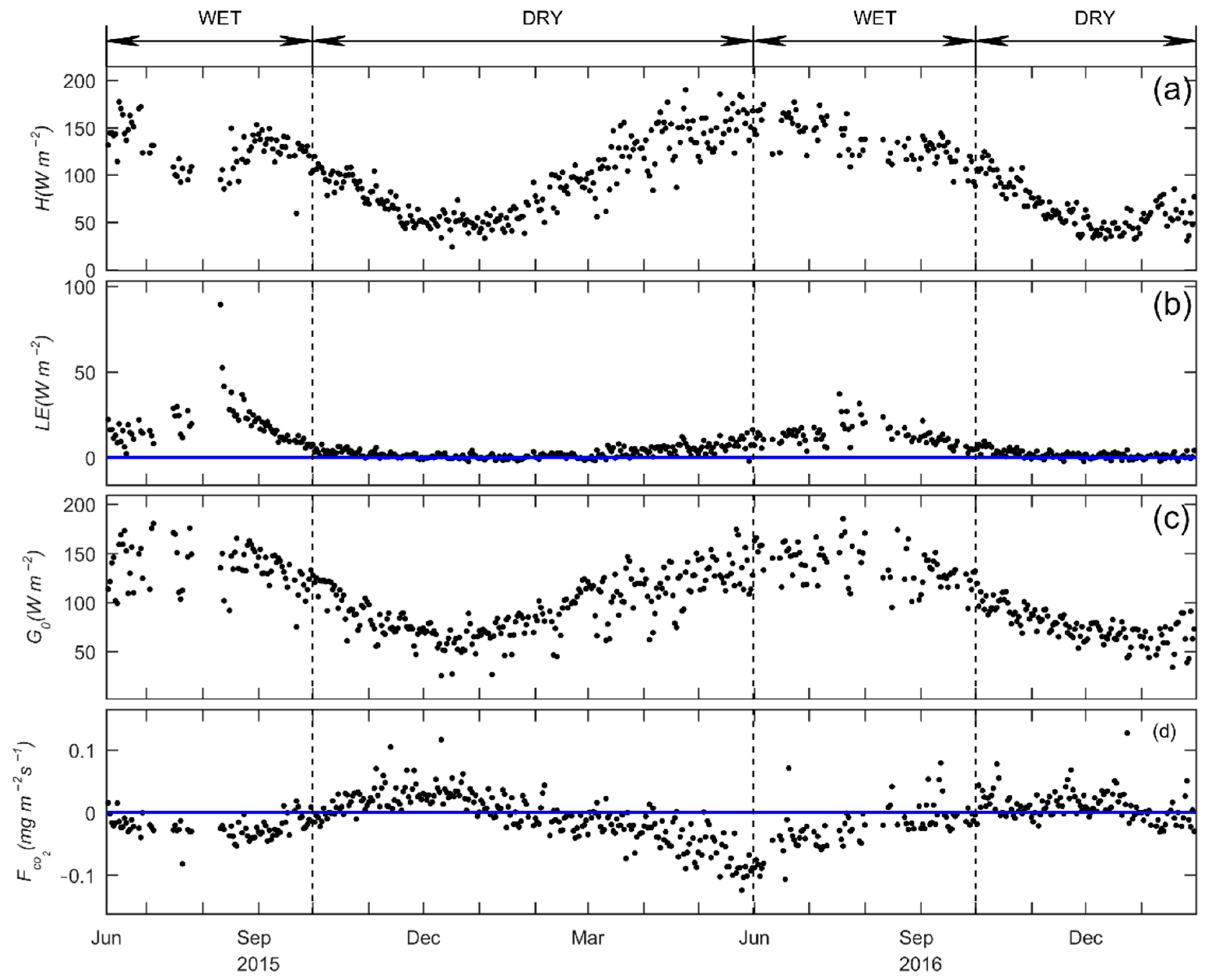
3.3.2. Heat and CO₂ Fluxes

Figure 6 shows the seasonal variations of daily daytime means of H, LE, G₀, and $F_{C{O}_2}$, all of which had remarkable seasonal variations. The maximum of the daily daytime mean H was shown in May and a little ahead of that of Rn, but the minimum was in December and consistent with that of Rn. In the year 2016, the maximum and minimum of the daily daytime mean H were 189.77 W m⁻² and 32.70 W m⁻², respectively. The daily daytime averaged LE was mostly within 10 W m⁻² in the dry season but could be larger than 30 W m⁻² in the wet season. The maximum daily daytime mean LE of 88.48 W m⁻² occurred in August 2015 associated with a precipitation event, which was much smaller than the observations at Lhasa in the central, Nyingchi, Wudaoliang, and Litang in the eastern, Haibei, Nagqu, and Tanggula in the northeastern TP, where the latent heat flux was generally larger than 100 W m⁻² in wet season [24,33,57,58,59,63,64]. The fluctuation of G₀ was well correlated with Rn. The daily daytime averaged G₀ was always positive showing that the land constantly absorbed heat in the daytime. In the year 2016, the maximum (minimum) daily daytime mean G₀ was in June (December) with a value of 185.28 W m⁻² (26.65 W m⁻²).

Daily daytime mean$F_{C{O}_2}$ was positive in late autumn and early winter but negative in late spring and early summer. The negative period was relatively longer and last about eight months (February 2016 to September 2016), while the positive period was short and last for about three months (October to December 2016). In the year 2016, the maximum (minimum) daily daytime mean $F_{C{O}_2}$ was in December (May) with a value of 0.13 mg m⁻² s⁻¹ (−0.13 mg m⁻² s⁻¹).

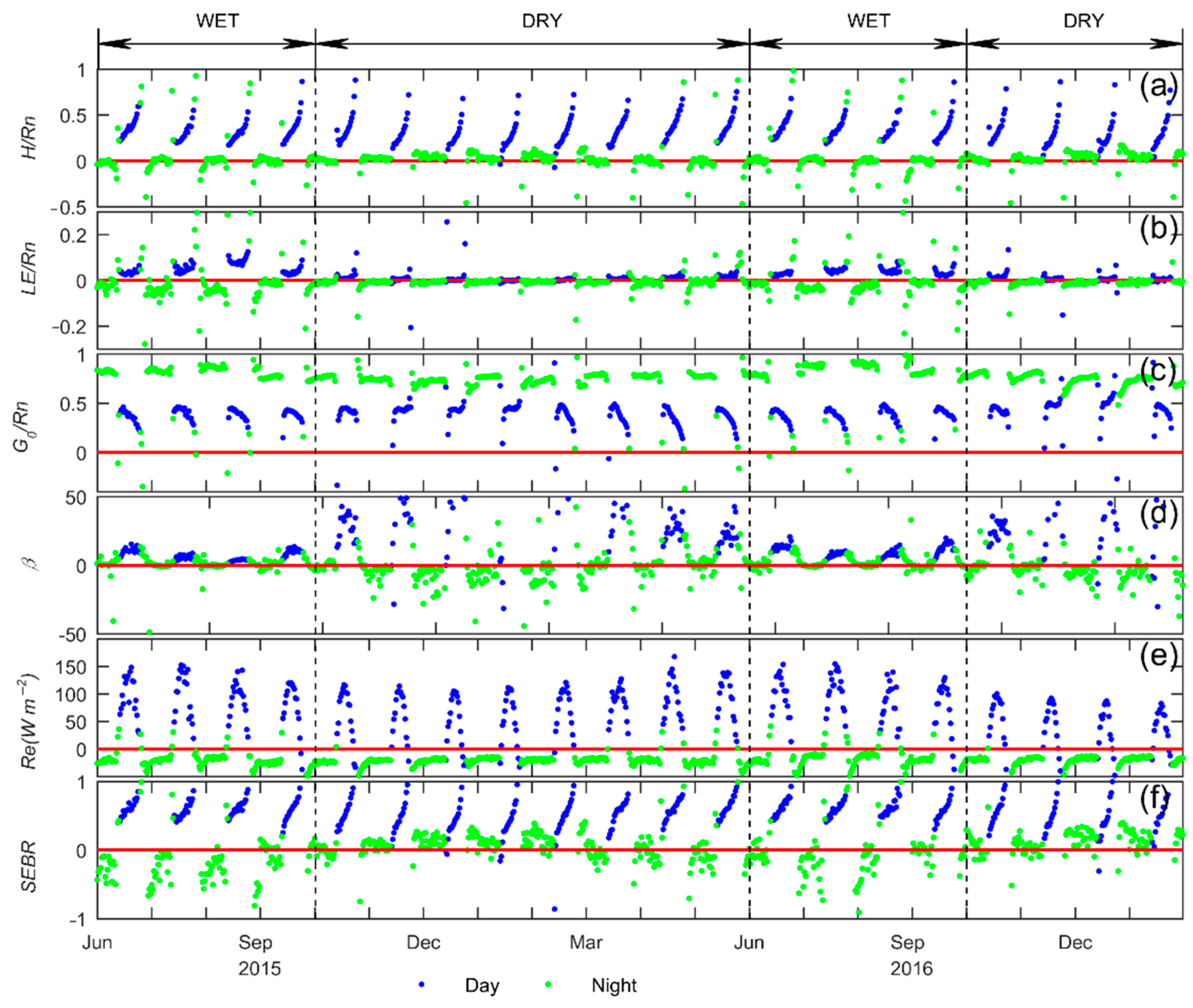
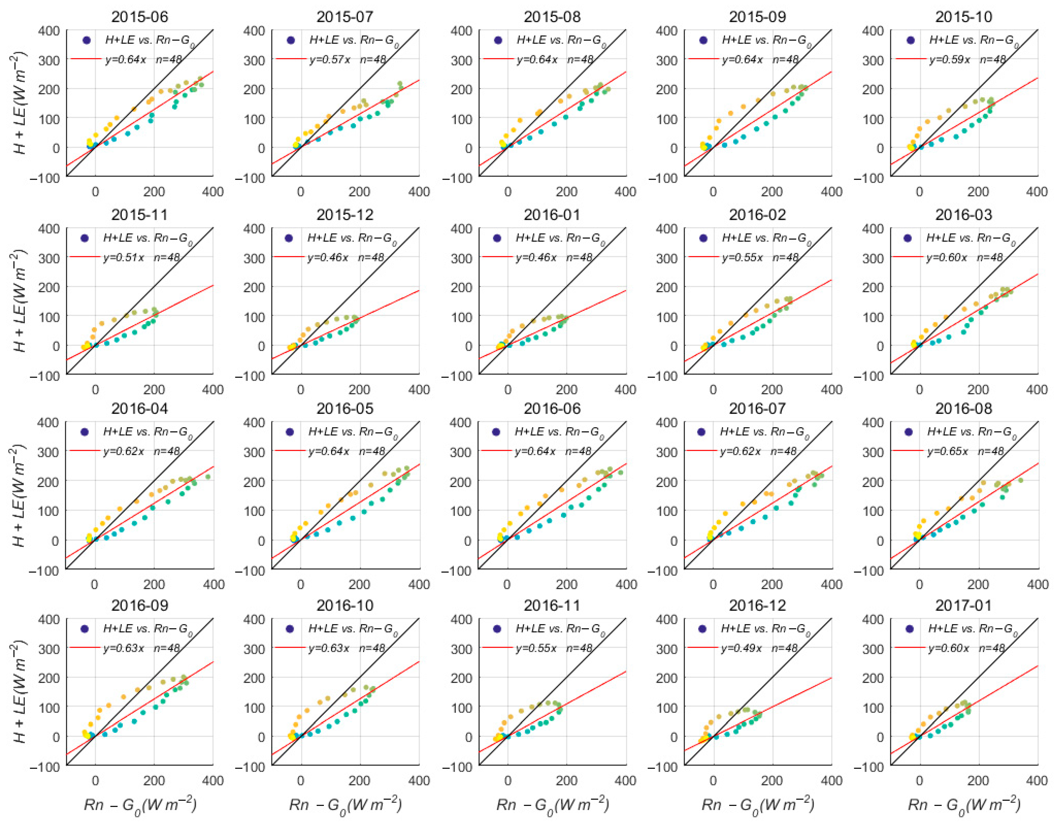
3.4. Energy Partitioning and Energy Balance Closure

To further understand the energy partitioning, the monthly averaged diurnal variation of H/Rn, LE/Rn, G₀/Rn, Bowen ratio (β = H/LE), Re and SEBR are shown in Figure 7. As H was relatively small in the nighttime, H/Rn was close to zero at night in all months. After sunrise, H/Rn started to increase. Further, the diurnal variation phase of H was about one hour behind that of Rn (not shown), H/Rn reached to near unity at the time of sunset. LE accounted for a very small amount of Rn at this site, and LE/Rn was mostly around zero in the dry season but fluctuated within ±0.25 in the wet season. Diurnal variation of LE/Rn from negative at night to positive in the daytime during the wet season was caused by the change of the sign of Rn. G₀/Rn was generally positive throughout the whole period. During the daytime, G₀/Rn had a quasi-sinusoidal fluctuation with a maximum of about 0.4–0.5 around noon, while during nighttime, G₀/Rn was generally invariant with a value of about 0.8–0.9 indicating that surface energy loss through radiation was mostly compensated by G₀. The absolute values of the Bowen ratio in this site could be extremely large (>50) in the dry season which was caused by the near-zero latent heat flux. While in Figure 7d, only the absolute values smaller than 50 are shown. In the wet season, diurnal quasi-sinusoidal fluctuations of β were found, with the maximum values shown around noon. Besides, the year-to-year difference was also presented and β in the wet season of 2016 was generally larger than that of 2015, which was related to higher rainfall quantity in 2015. In the dry season, at night, H was close to zero so that β also fluctuated around zero, but during the daytime, its absolute values could reach more than 50 and its sign was determined by the direction of the near-zero latent heat flux. Respondent to the quasi-sinusoidal variation of DSR, the residual energy Re in the daytime had also a quasi-sinusoidal fluctuation with a maximum of about 100–150 W m⁻² around noon and a minimum reaching −50 W m⁻² at sunset, while at night it was generally invariant around −20 W m⁻². SEBR showed significant diurnal variation as well. It was small and could be even negative in the nighttime, but after sunrise, it started to increase and reaching unity at sunset. The mean SEBR in the total period was 0.57, which was similar to but a little smaller than the finding of Xin et al. (0.65 from July to September) [34]. Many influencing factors contributed to the large Re and small SEBR. For example, the uncertainties caused by H and LE instrumental errors. Xin et al. pointed out that the uncertainties of Re caused by H and LE instrumental errors were generally smaller during the nighttime than those during the daytime, and the relative instrumental error in measuring H was nearly 12.8% whereas that for LE was 12.5% with the highest value reaching 22.9% [34]. Xin et al. also indicated that the soil heat storage term represented a significant source of uncertainty (~10%) to close the surface energy budget, which was affected by the soil respiration, heat storage in canopy, phase change of water in the soil, energy loss due to advection, while all of them were neglected in this study due to the difficulties in measurement. Further, even if the measurement’s uncertainties could be reduced to zero, and all energy exchange processes and losses were measured precisely, the residual energy still could not be close to zero because of the lagging of the diurnal wave phases of G₀ to those of H and LE [65,66,67]. In our study, in addition to the above reasons, the following factors could also contribute to the non-closure: (1) The effect of freezing and thawing on the calculation of G₀, as the latent heat related to the water phase change in the soil was not considered. (2) The lower moisture content in the atmosphere. The moisture was very low in our study area, which might lead to significant uncertainty in the measurement of latent heat. (3) The complex composition of soil surface. We regarded the soil here as uniform sand to set the relevant soil parameters (e.g., saturated soil moisture and soil volume heat capacity). However, the underlying surface in the observation site was a mixture of sand and a small number of pebbles. (4) The influence of nearby buildings and human activities on the site.

As shown in Figure 8, SEBR went through a regular diurnal cycle in every month, starting from roughly the origin point at morning then to the left of 1:1 line, it crossed the 1:1 line around noon and to its right at afternoon, at the same time both turbulent heat fluxes (H + LE) and surface available energy (Rn − G₀) reached their maxima, then at night, it retreated to the origin point gradually. Seasonal variation was also presented, and in summer months, the slopes of the fitting curve were mostly above 0.6, but in winter months, they were around 0.5.

4. Summary and Conclusions

To examine the land–atmosphere interaction and understand the surface energy partitioning and CO₂ exchange over western TP, continuous measurements on radiation and turbulent heat fluxes, soil heat fluxes and CO₂ flux were conducted from June 2015 through January 2017 at Shiquanhe (32.50° N, 80.08° E, 4279.3 m above sea level) in the western Tibetan Plateau.

The Shiquanhe site was dominated by weak south-westerlies (generally below 3 m s⁻¹) and could be divided into a wet (June to September) and a dry season (October to May). All the rainfall was in the wet season, and the 30-min specific humidity reached 12 g kg⁻¹ in the wet season but kept less than 2 g kg⁻¹ in the dry season. Diurnal variations of the four radiation components, three heat fluxes, and CO_2, flux were found. In 2016, the magnitudes of the monthly averaged diurnal variations for DSR, USR, and ULR were the largest in June (smallest in December), with values of 1078.24, 206.06, and 218.88 W m⁻² (632.14, 142.75, and 132.67 W m⁻²), respectively. However, DLR had relatively weaker diurnal fluctuations of about 50 W m⁻² all over the year. Due to the small albedo here (0.2–0.4), Rn was mainly affected by DSR and had a diurnal variation magnitude of about 730 W m⁻². For H, large positive values in the daytime (over 200 and 100 W m⁻² in summer and winter, respectively) but near zero or very few negative values in nighttime showed. LE at the Shiquanhe site was extremely small in the dry season (within 5 W m⁻²) but could reach 42.2 W m⁻² in the wet season. G₀ had a significant diurnal variation with the diurnal maximum values (about 140~240 W m⁻²) at noon and diurnal minimum values (about −50 ~ −100 W m⁻²) at midnight during the observation period. For $F_{C{O}_2}$, diurnal variation of respiration caused by the biological and chemical processes within the soil was found, large absorption (release) of CO₂ around 0.1 mg m⁻² s⁻¹ occurred in the afternoon of summer (midnight of winter). However, from a yearly perspective, the absorption and release generally canceled out, and yearly average of $F_{C{O}_2}$ in 2016 was close to zero.

Seasonal variations also appeared for the daily daytime (10:00–19:00 local time) mean radiation, turbulent, and soil heat fluxes, and the maxima were all in summer and minimum in winter. DSR, USR, and ULR generally shared the same phase of seasonal variation and had their maxima (minima) in June (December) with values of 885.52, 181.15, and 530.65 W m⁻² (178.39, 40.42, and 286.95 W m⁻²), respectively. While DLR was one to two months behind and had its maximum (minimum) in August (January) with values of 336.53 W m⁻² (151.34 W m⁻²). Rn was also slightly behind the phase of DSR, with its maximum (minimum) value of 465.41 W m⁻² (68.79 W m⁻²) shown in July (December). The daily daytime mean albedo had only slight seasonal variation and fluctuated within 0.20 ± 0.03, and its maximum was in winter associating with the drier soil. The maximum (minimum) daily daytime mean H was shown in May (December) with a value of 189.77 and 32.70 W m⁻² in 2016, while the maximum LE larger than 30 W m⁻² generally occurred in July or August associated with precipitation events. Daily daytime mean G₀ was always positive, and its yearly maximum (minimum) in 2016 occurred in June (December) with a value of 185.28 W m⁻² (26.65 Wm⁻²). In the daytime, the soil absorbed (released) CO₂ around May (December) at a rate of 0.13 mg m⁻² s⁻¹.

Diurnal and seasonal variation of H/Rn, LE/Rn, G₀/Rn, Bowen ratio (β = H/LE), Re and SEBR are also presented in this study. H/Rn was relatively large and could reach unity at the time of sunset, while LE/Rn was mostly around zero in the dry season but fluctuated within ±0.25 in the wet season. G₀/Rn was about 0.4–0.5 around noon and 0.8–0.9 at midnight. β had extremely large absolute values (>50) because of the near-zero of LE in the dry season, while in the wet season, it was within 10–50 at noon. Re in the daytime had a maximum of about 100-150 W m⁻² around noon and a minimum reaching −50 W m⁻² at sunset, and at night it was generally invariant around −20 W m⁻². The mean SEBR in the total period was 0.58. It went through both regular diurnal cycle and season variation, and in summer months, the slopes of the fitting curve were mostly above 0.6, but in winter months, they were around 0.5. The measurement errors of the fluxes, the effects of frozen soil on the calculation of G₀, the lower moisture content in the atmosphere, the complex composition of the soil surface, and the influence of nearby buildings and human activities were the possible reasons to the small SEBR.

Comparing the results from the Shiquanhe site with the central and eastern TP sites [24,33,57,58,59,63,64], it could be found that (1) they all generally had similar seasonal and diurnal variation of the fluxes, (2) caused by the low rainfall quantity, LE at Shiquanhe (daily daytime mean always less than 90 W m⁻²) was distinctively smaller than the central and eastern TP sites during the wet season, where the latent heat flux was generally larger than 100 W m⁻², and (3) affected by various factors, the residual energy was comparatively larger at Shiquanhe, which led to a small surface energy balance ratio.

References

1. Ye, D.Z.; Gao, Y.X. Meteorology of the Qinghai–Xizang Plateau; Science Press: Beijing, China, 1979; pp. 1–278. (In Chinese) [Google Scholar]
2. Luo, H.B.; Yanai, M. The large-scale circulation and heat sources over the Tibetan Plateau and surrounding areas during the early summer of 1979. Part Ⅱ: Heat and moisture budgets. Mon. Weather Rev. 1984, 112, 966–989. [Google Scholar] [CrossRef] [Green Version]
3. Yanai, M.; Li, C.F.; Song, Z.S. Seasonal heating of the Tibetan Plateau and its effects on the evolution of the Asian summer monsoon. J. Meteor. Soc. Jpn. Ser. II 1992, 70, 319–351. [Google Scholar] [CrossRef] [Green Version]
4. Wu, G.X.; Zhang, Y.S. Tibetan Plateau forcing and the timing of the monsoon onset over South Asia and the South China Sea. Mon. Weather Rev. 1998, 126, 913–927. [Google Scholar] [CrossRef]
5. Zhao, P.; Chen, L.X. Climatic features of atmospheric heat source/sink over the Qinghai–Xizang Plateau in 35 years and its relation to rainfall in China. Sci. China Earth Sci. 2001, 44, 858–864. [Google Scholar] [CrossRef]
6. Zhao, P.; Chen, L.X. Role of atmospheric heat source/sink over the Qinghai–Xizang Plateau in quasi-4-year oscillation of atmosphere–land–ocean interaction. Chin. Sci. Bull. 2001, 46, 241–245. [Google Scholar] [CrossRef]
7. Wu, G.X.; Liu, Y.M.; Wang, T.M.; Wan, R.J.; Liu, X.; Li, W.P.; Wang, Z.Z.; Zhang, Q.; Duan, A.M.; Liang, X.Y. The influence of mechanical and thermal forcing by the Tibetan Plateau on Asian climate. J. Hydrom. 2007, 8, 770–789. [Google Scholar] [CrossRef] [Green Version]
8. Xu, X.D.; Lu, C.G.; Shi, X.H.; Gao, S.T. World water tower: An atmospheric perspective. Geophys. Res. Lett. 2008, 35, L20815. [Google Scholar] [CrossRef]
9. Zhou, X.J.; Zhao, P.; Chen, J.M.; Chen, L.X.; Li, W.L. Impacts of thermodynamic processes over the Tibetan Plateau on the Northern Hemispheric climate. Sci. China Earth Sci. 2009, 52, 1679–1693. [Google Scholar] [CrossRef]
10. Boos, W.R.; Kuang, Z.M. Dominant control of the South Asian monsoon by orographic insulation versus plateau heating. Nature 2010, 463, 218–222. [Google Scholar] [CrossRef]
11. Wu, G.X.; Liu, Y.M.; He, B.; Bao, Q.; Duan, A.; Jin, F.F. Thermal controls on the Asian summer monsoon. Sci. Rep. 2012, 2, 404. [Google Scholar] [CrossRef] [Green Version]
12. Zhao, P.; Wang, B.; Liu, J.P.; Zhou, X.J.; Chen, J.M.; Nan, S.L.; Liu, G.; Xiao, D. Summer precipitation anomalies in Asia and North America induced by eurasian non-monsoon land heating versus ENSO. Sci. Rep. 2016, 6, 21346. [Google Scholar] [CrossRef] [PubMed] [Green Version]
13. Zhao, P.; Xu, X.; Chen, F.; Guo, X.; Zheng, X.; Liu, L.; Hong, Y.; Li, Y.; La, Z.; Peng, H.; et al. The third atmospheric scientific experiment for understanding the earth–atmosphere coupled system over the Tibetan plateau and its effects. Bull. Am. Meteorol. Soc. 2018, 99, 757–776. [Google Scholar] [CrossRef]
14. Zhao, P.; Li, Y.; Guo, X.; Xu, X.; Liu, Y.; Tang, S.; Xiao, W.; Shi, C.; Ma, Y.; Yu, X.; et al. The Tibetan Plateau surface-atmosphere coupling system and its weather and climate effects: The Third Tibetan Plateau Atmospheric Science Experiment. J. Meteorol. Res. 2019, 33, 375–399. [Google Scholar] [CrossRef]
15. Ye, D.Z. Some characteristics of the summer circulation over the Qinghai–Xizang (Tibet) Plateau and its neighborhood. Bull. Am. Meteorol. Soc. 1981, 62, 14–19. [Google Scholar] [CrossRef] [Green Version]
16. Ye, D.Z.; Wu, G.X. The role of the heat source of the Tibetan Plateau in the general circulation. Meteorol. Atmos. Phys. 1998, 67, 181–198. [Google Scholar] [CrossRef]
17. Shi, Y.F.; Yu, G.; Liu, X.D.; Li, B.Y.; Yao, T.D. Reconstruction of the 30–40 ka BP enhanced India monsoon climate based on geological record from the Tibetan Plateau. Palaeogeogr. Palaeoclimatol. Palaeoecol. 2001, 169, 69–83. [Google Scholar] [CrossRef]
18. Hsu, H.H.; Liu, X. Relationship between the Tibetan Plateau heating and East Asian summer monsoon rainfall. Geophys. Res. Lett. 2003, 30, 2066. [Google Scholar] [CrossRef] [Green Version]
19. Sato, T.; Kimura, F. How does the Tibetan Plateau affect the transition of Indian monsoon rainfall? Mon. Weather Rev. 2007, 135, 2006–2015. [Google Scholar] [CrossRef]
20. Ma, Y.M.; Kang, S.C.; Zhu, L.P.; Xu, B.Q.; Tian, L.D.; Yao, T.D. Tibetan observation and research platform: Atmosphere–land interaction over a heterogeneous landscape. Bull. Am. Meteorol. Soc. 2008, 89, 1487–1492. [Google Scholar]
21. Cui, X.F.; Graf, H.F. Recent land cover changes on the Tibetan Plateau: A review. Clim. Change 2009, 94, 47–61. [Google Scholar] [CrossRef] [Green Version]
22. Yang, K.; Ye, B.S.; Zhou, D.G.; Wu, B.Y.; Foken, T.; Qin, J.; Zhou, Z.Y. Response of hydrological cycle to recent climate changes in the Tibetan Plateau. Clim. Change 2011, 109, 517–534. [Google Scholar] [CrossRef]
23. Duan, A.M.; Wu, G.X.; Liu, Y.M.; Ma, Y.M.; Zhao, P. Weather and climate effects of the Tibetan Plateau. Adv. Atmos. Sci. 2012, 29, 978–992. [Google Scholar] [CrossRef]
24. Gu, L.L.; Yao, J.M.; Hu, Z.Y.; Zhao, L. Comparison of the surface energy budget between regions of seasonally frozen ground and permafrost on the Tibetan Plateau. Atmos. Res. 2015, 153, 553–564. [Google Scholar] [CrossRef]
25. Karl, T.R.; Trenberth, K.E. Modern global climate change. Science 2003, 302, 1719–1723. [Google Scholar] [CrossRef] [Green Version]
26. Tanaka, K.; Tamagawa, I.; Ishikawa, H.; Ma, Y.; Hu, Z. Surface energy budget and closure of the eastern Tibetan Plateau during the GAME-Tibet IOP 1998. J. Hydrol. 2003, 283, 169–183. [Google Scholar] [CrossRef]
27. Choi, T.; Hong, J.; Kim, J.; Lee, H.; Asanuma, J.; Ishikawa, H.; Tsukamoto, O.; Gao, Z.Q.; Ma, Y.M.; Ueno, K.; et al. Turbulent exchange of heat, water vapor, and momentum over a Tibetan prairie by eddy covariance and flux variance measurements. J. Geophys. Res. Atmos. 2004, 109, D21. [Google Scholar] [CrossRef]
28. Gu, S.; Tang, Y.H.; Cui, X.Y.; Kato, T.; Du, M.Y.; Li, Y.N.; Zhao, X.Q. Energy exchange between the atmosphere and a meadow ecosystem on the Qinghai–Tibetan Plateau. Agric. For. Meteorol. 2004, 129, 175–185. [Google Scholar] [CrossRef]
29. Ma, W.Q.; Ma, Y.M. The annual variations on land surface energy in the northern Tibetan Plateau. Environ. Geol. 2007, 51, 1465. [Google Scholar]
30. Yao, J.M.; Zhao, L.; Ding, Y.J.; Gu, L.L.; Jiao, K.Q.; Qiao, Y.P.; Wang, Y.Q. The surface energy budget and evapotranspiration in the Tanggula region on the Tibetan Plateau. Cold Reg. Sci. Technol. 2007, 52, 326–340. [Google Scholar] [CrossRef]
31. Guo, D.L.; Yang, M.X.; Wang, H.J. Characteristics of land surface heat and water exchange under different soil freeze/thaw conditions over the central Tibetan Plateau. Hydrol. Process. 2011, 25, 2531–2541. [Google Scholar] [CrossRef]
32. Yang, K.; He, J.; Tang, W.J.; Qin, J.; Cheng, C.C. On downward shortwave and longwave radiations over high altitude regions: Observation and modeling in the Tibetan Plateau. Agric. For. Meteorol. 2010, 150, 38–46. [Google Scholar] [CrossRef]
33. You, Q.; Xue, X.; Peng, F.; Dong, S.; Gao, Y. Surface water and heat exchange comparison between alpine meadow and bare land in a permafrost region of the Tibetan Plateau. Agric. For. Meteorol. 2017, 232, 48–65. [Google Scholar] [CrossRef]
34. Xin, Y.F.; Chen, F.; Zhao, P.; Barlage, M.; Blanken, P.; Chen, Y.L.; Wang, Y.J. Surface energy balance closure at ten sites over the Tibetan plateau. Agric. For. Meteorol. 2018, 259, 317–328. [Google Scholar] [CrossRef]
35. Kljun, N.; Calanca, P.; Rotach, M.W.; Schmid, H.P.A. Simple two-dimensional parameterization for Flux Footprint Prediction (FFP). Geosci. Model Dev. 2015, 8, 3695–3713. [Google Scholar] [CrossRef] [Green Version]
36. Vickers, D.; Mahrt, L. Quality control and flux sampling problems for tower and aircraft data. J. Atmos. Ocean. Technol. 1997, 14, 512–526. [Google Scholar] [CrossRef]
37. Tanner, C.B.; Thurtell, G.W. Anemoclinometer Measurements of Reynolds Stress and Heat Transport in the Atmospheric Surface Layer; University of Wisconsin: Madison, WI, USA, 1969; p. 82. [Google Scholar]
38. Webb, E.K.; Pearman, G.I.; Leuning, R. Correction of flux measurements for density effects due to heat and water vapor transfer. Q. J. R. Meteorol. Soc. 1980, 106, 85–100. [Google Scholar] [CrossRef]
39. Moncrieff, J.; Clement, R.; Finnigan, J.; Meyers, T. Averaging, Detrending, and Filtering of Eddy Covariance Time Series. In Handbook of Micrometeorology: A Guide for Surface Flux Measurement and Analysis; Lee, X., Massman, W., Law, B., Eds.; Kluwer Academic: Dordrecht, The Netherlands, 2004; pp. 7–30. [Google Scholar]
40. Zhao, X.R.; Sheng, Z.; Li, J.W.; Yu, H.; Wei, K.J. Determination of the “wave turbopause” using a numerical differentiation method. J. Geophys. Res.: Atmos. 2019, 124, 10592–10607. [Google Scholar] [CrossRef]
41. He, Y.; Sheng, Z.; He, M. Spectral Analysis of Gravity Waves from Near Space High-Resolution Balloon Data in Northwest China. Atmosphere 2020, 11, 133. [Google Scholar] [CrossRef] [Green Version]
42. Van Wijk, W. Physics of plant environment. Soil Sci. 1964, 98, 69. [Google Scholar] [CrossRef]
43. Garratt, J.R. The Atmospheric Boundary Layers; Cambridge University Press: New York, NY, USA, 1992; p. 316. [Google Scholar]
44. Franssen, H.J.H. Energy balance closure of eddy-covariance data: A multisite analysis for European FLUXNET stations. Agric. For. Meteorol. 2010, 150, 1553–1567. [Google Scholar] [CrossRef]
45. Harazono, Y.; Kim, J.; Miyata, A.; Choi, T.; Yun, J.I. Measurement of energy budget components during the International Rice Experiment (IREX) in Japan. Hydrol. Process. 1998, 12, 2018–2092. [Google Scholar] [CrossRef]
46. Burba, G.; Verma, B.S.; Kim, J. Surface energy fluxes of Phragmites australis in a prairie wetland. Agric. For. Meteorol. 1999, 94, 31–51. [Google Scholar] [CrossRef]
47. Heitman, J.L.; Xiao, X.; Horton, R.; Sauer, T. Sensible heat measurements indicating depth and magnitude of subsurface soil water evaporation. Water Resour. Res. 2008, 44, W00D05. [Google Scholar] [CrossRef] [Green Version]
48. Heitman, J.L.; Horton, R.; Sauer, T.J.; Desutter, T.M. NOTES AND CORRESPONDENCE: Sensible Heat Observations Reveal Soil-Water Evaporation Dynamics. J. Hydrometeorol. 2008, 9, 165–171. [Google Scholar] [CrossRef] [Green Version]
49. Heitman, J.L.; Horton, R.; Sauer, T.J.; Ren, T.S.; Xiao, X. Latent heat in soil heat flux measurements. Agric. For. Meteorol. 2010, 150, 1147–1153. [Google Scholar] [CrossRef] [Green Version]
50. Foken, T. The energy balance closure problem: An overview. Ecol. Appl. 2008, 18, 1351–1367. [Google Scholar] [CrossRef]
51. Gu, J.; Smith, E.A.; Merritt, J.D. Testing energy balance closure with GOES-retrieved net radiation and in situ measured eddy correlation fluxes in BOREAS. J. Geophys. Res. 1999, 104, 27881–27893. [Google Scholar] [CrossRef]
52. Wilson, K.B. Energy balance closure at FLUXNET sites. Agric. For. Meteorol. 2002, 113, 223–234. [Google Scholar] [CrossRef] [Green Version]
53. McGloin, R.; Šigut, L.; Havránková, K.; Dušek, J.; Pavelka, M.; Sedlák, P. Energy balance closure at a variety of ecosystems in Central Europe with contrasting topographies. Agric. For. Meteorol. 2018, 248, 418–431. [Google Scholar] [CrossRef]
54. Ohtaki, E. Application of an inferred carbon dioxide and humidity instrument to studies of turbulent transport. Bound. Lay. Meteorol. 1984, 29, 85–107. [Google Scholar] [CrossRef]
55. Ohtaki, E.; Matsui, T. Infrared device for simultaneous measurement of atmospheric carbon dioxide and water vapor. Bound. Lay. Meteorol. 1982, 24, 109–119. [Google Scholar] [CrossRef]
56. Desai, A.R. Influence of vegetation and surface forcing on carbon dioxide fluxes across the Upper Midwest, USA: Implications for regional scaling. Agric. For. Meteorol. 2008, 148, 288–308. [Google Scholar] [CrossRef]
57. Ma, Y.; Fan, S.; Ishikawa, H.; Tsukamoto, O.; Yao, T.; Koike, T.; Zuo, H.; Hu, Z.; Su, Z. Diurnal and inter-monthly variation of land surface heat fluxes over the central Tibetan Plateau area. Theor. Appl. Climatol. 2005, 80, 259–273. [Google Scholar] [CrossRef]
58. Zhao, X.; Peng, B.; Qin, N.; Wang, W. Characteristics of Energy Transfer and Micrometeorology in Surface Layer in Different Areas of Tibetan Plateau in Summer. Plateau Mt. Meteorol. Res. 2011, 31, 6–11. [Google Scholar]
59. Zhao, X.; Li, Y. Seasonal Characteristics of Turbulent Flux and Meteorology Elements in the Atmosphere Surface Layer over the Alpine Meadow on Eastern Slop of Tibetan Plateau. Plateau Mt. Meteorol. Res. 2011, 31, 12–17. [Google Scholar]
60. Wohlfahrt, G.; Fenster maker, L.F. A Large annual net ecosystem CO2 uptake of a Mojave Desert ecosystem. Glob.Change Biol. 2008, 1497, 1475–1487. [Google Scholar] [CrossRef]
61. Xie, J.; Li, Y. CO2 absorption by alkaline soils and its implication to the global carbon cycle. Environ. Geol. 2009, 56, 953–961. [Google Scholar] [CrossRef]
62. Mamtimin, A. Study on Characteristics and Influencing Factors of Carbon Exchange of Desert Area in Xinjiang; NUIST: Nanjing, China, 2015. [Google Scholar]
63. Yang, K.; Koike, T. Satellite monitoring of the surface water and energy budget in the central Tibetan Plateau. Adv. Atmos. Sci. 2008, 25, 974–985. [Google Scholar] [CrossRef]
64. Guo, D.; Yang, M.; Wang, H. Sensible and latent heat flux response to diurnal variation in soil surface temperature and moisture under different freeze/thaw soil conditions in the seasonal frozen soil region of the central Tibetan Plateau. Environ. Earth Sci. 2011, 63, 97–107. [Google Scholar] [CrossRef]
65. Gao, Z. Determination of soil heat flux in a Tibetan short-grass prairie. Boundary-Layer Meteorol. 2005, 114, 165–178. [Google Scholar] [CrossRef]
66. Gao, Z.; Bian, L.; Hu, Y.; Wang, L.; Fan, J. Determination of soil temperature in an arid region. J. Arid Environ. 2007, 71, 157–168. [Google Scholar] [CrossRef]
67. Gao, Z.; Horton, R.; Liu, H. Impact of wave phase difference between surface soil heat flux and soil surface temperature on land surface energy balance closure. J. Geophys. Res. 2010, 115, D16112. [Google Scholar] [CrossRef]
Figure 1. (a) The geographical location, (b) local topography, (c) underlying surface and footprint of surface turbulent fluxes, and (d) observation tower and instruments at the Shiquanhe site. The satellite map was from the website: https://www.amap.com.
Atmosphere 11 00260 g001
Figure 2. The (a) daily mean wind speed (WS in m s−1), (b) daily mean wind direction (WD in degree), (c) daily mean air temperature (Tair in K), (d) daily mean specific humidity (q in g kg−1), (e) daily accumulated precipitation (Prec. in mm), and (f) daily mean air pressure (P in hPa) at the Shiquanhe site from 9 June 2015 through 31 January 2017.
Atmosphere 11 00260 g002
Figure 3. The monthly averaged diurnal variations of (a) downward shortwave radiation (DSR in W m−2), (b) upward shortwave radiation (USR in W m−2), (c) downward longwave radiation (DLR in W m−2), (d) upward longwave radiation (ULR in W m−2), (e) net radiation (Rn in W m−2) and (f) surface albedo (defined as the ratio of USR to DSR) during the period from June 2015 to January 2017 at the Shiquanhe site.
Atmosphere 11 00260 g003
Figure 4. The monthly averaged diurnal variations of (a) sensible heat flux (H in W m−2), (b) latent heat flux (LE in W m−2), (c) soil heat flux (G0 in W m−2) and (d) CO2 flux ( F C O 2 in mg m−2 s−1) during the period from June 2015 to January 2017 at the Shiquanhe site.
Atmosphere 11 00260 g004
Figure 5. Daily daytime (10:00–19:00 local time) means of (a) downward shortwave radiation (DSR in W m−2), (b) upward shortwave radiation (USR in W m−2), (c) downward longwave radiation (DLR in W m−2), (d) upward longwave radiation (ULR in W m−2), (e) net radiation (Rn in W m−2) and (f) surface albedo during the observation period from June 2015 to January 2017 at the Shiquanhe site.
Atmosphere 11 00260 g005
Figure 6. Daily daytime (10:00 – 19:00 local time) means of (a) sensible heat flux (H in W m2), (b) latent heat flux (LE in W m2), (c) soil heat flux (G0 in W m2), and (d) CO2 flux ( F C O 2 in mg m−2 s−1) from June 2015 to January 2017 at the Shiquanhe site.
Atmosphere 11 00260 g006
Figure 7. The monthly averaged diurnal variations of H/Rn, LE/Rn, G0/Rn, Bowen ratio (β), Re, and SEBR. Blue and green dots indicate daytime (10:00–19:00 local time) and nighttime (19:00–10:00 local time), respectively.
Atmosphere 11 00260 g007
Figure 8. Monthly averaged diurnal variations of turbulent heat fluxes (H + LE) versus surface available energy (RnG0) for each of the months in the observation period. Yellow and green dots indicate daytime (10:00–19:00 local time) and nighttime (19:00–10:00 local time), respectively.
Atmosphere 11 00260 g008