Article

Parameterization of Wave-Induced Mixing Using the Large Eddy Simulation (LES) (I)

1
School of Marine Sciences, Nanjing University of Information Science & Technology, Nanjing 210044, China
2
Southern Laboratory of Ocean Science and Engineering Guangdong Laboratory, Zhuhai 519082, China
3
Laboratory for Regional Oceanography and Numerical Modeling, Qingdao National Laboratory for Marine Science and Technology, Qingdao 266061, China
4
First Institute of Oceanography, Ministry of Natural Resources, Qingdao 266061, China
5
Key Laboratory of Marine Science and Numerical Modeling, Ministry of Natural Resources, Qingdao 266061, China
6
College of Ocean Science and Engineering, Shandong University of Science and Technology, Qingdao 266590, China
*
Author to whom correspondence should be addressed.
Atmosphere 2020, 11(2), 207; https://doi.org/10.3390/atmos11020207
Submission received: 5 January 2020 / Revised: 10 February 2020 / Accepted: 12 February 2020 / Published: 15 February 2020
(This article belongs to the Section Biosphere/Hydrosphere/Land–Atmosphere Interactions)

Abstract

:
Turbulent motions in the thin ocean surface boundary layer control exchanges of momentum, heat and trace gases between the atmosphere and ocean. However, present parametric equations of turbulent motions that are applied to global climate models result in systematic or substantial errors in the ocean surface boundary layer. Significant mixing caused by surface wave processes is missed in most parametric equations. A Large Eddy Simulation model is applied to investigate the wave-induced mixed layer structure. In the wave-averaged equations, wave effects are calculated as Stokes forces and breaking waves. To examine the effects of wave parameters on mixing, a series of wave conditions with varying wavelengths and heights are used to drive the model, resulting in a variety of Langmuir turbulence and wave breaking outcomes. These experiments suggest that wave-induced mixing is more sensitive to wave heights than to the wavelength. A series of numerical experiments with different wind intensities-induced Stokes drifts are also conducted to investigate wave-induced mixing. As the wind speed increases, the influence depth of Langmuir circulation deepens. Additionally, it is observed that breaking waves could destroy Langmuir cells mainly at the sea surface, rather than at deeper layers.

1. Introduction

The ocean mixed layer is central to heat and momentum exchange processes between the upper ocean and the atmosphere. Waves play an integral part as they modulate those exchanges across the air-sea interface and consequently, their influence on mixed layer dynamics and structure cannot be ignored [1]. Specifically, as wind blows over the ocean surface, momentum is transported into the ocean, resulting in enhancement of both mixing and turbulent kinetic energy. Stokes drift also plays a role in modulating upper-ocean turbulence through large-scale Coriolis-Stokes and small-scale Stokes-vortex forces. It is the interaction of Stokes drift with wind-driven surface shear flow that induces Langmuir circulation (LC) formation [2]. As one of the most significant features of the mixed layer, LC appears as an array of alternating horizontal roll vortices, whose axes are roughly parallel to the wind direction [3,4,5]. LC could enhance the vertical mixing and alter vertical profiles of temperature and velocity [6,7,8,9], making it crucial in upper ocean studies. Upper ocean turbulence is also affected by Langmuir turbulence and is primarily generated by surface waves. The depth at which LC the upper ocean is largely determined by the Stokes drift e-folding depth and the mixed layer thickness [10,11]. The injection of turbulent kinetic energy from breaking surface gravity waves provides another significant source of upper-ocean turbulence [12]. Increased turbulence due to breaking waves (BW) decays following reductions in significant wave heights [13,14].
The importance of wave-induced mixing is demonstrated in upper-ocean mixed layer studies. However, most turbulence schemes such as the Mellor-Yamada [15] or K-profile [16] parameterizations do not account for wave processes. These turbulence models are handicapped by the failure to include mixed layer physical processes such as BW and LC. This results in ocean mixed layer models producing too shallow mixed layer depths in high-latitude oceans (especially the Southern Ocean) [17,18,19,20,21,22] and highly diffused thermoclines in tropical oceans [8,23,24,25,26], leading to weaker El Niño in climate models [27]. Furthermore, the principal way in which waves influence the oceanic circulation is through wave-induced vertical mixing, which is currently limited by model resolution, thus necessitating parameterization [28,29,30]. To more realistically reproduce the upper ocean in ocean general circulation models, a number of ocean mixed layer models have been proposed [28,29,30,31,32,33,34,35,36,37,38,39]. For example, a parameterization scheme including wave-induced mixing is proposed to modify current Mellor-Yamada and K-profile parameterization turbulence models [36,40]. The comparison of numerical results with observations demonstrates the importance of the inclusion of wave-induced mixing as simulations of sea surface temperatures are significantly improved when wave-induced mixing is considered.
A large number of wave-induced mixing studies employs the Large Eddy Simulation (LES) models. First pioneered by Skyllingstad and Denbo [41] in their application of LES to investigate Langmuir turbulence, additional researches have also employed LES in studies on the influence of LC and BW near the ocean surface [7], and momentum injection induced by BW in the presence of Langmuir turbulence in the planetary boundary layer [7,26,42,43]. Sullivan et al. [44] indicates that the resonant wind and current rotation may deepen the mixed layer [45,46]. Kukulka and Brunner [47], based on wave-averaged Navier-Stokes equations, used LES to study the influence of equilibrium wind-waves on vertical tracer distributions through an investigation of passive buoyant tracers in the ocean surface boundary layer. Brunner et al. [48] indicates that Langmuir turbulence substantially increases turbulent transport in the ocean surface boundary layer.
In this study and a forthcoming article (the second part of the study), the LES model is used to investigate the wave-induced mixing and its parameterization. Innovating through delving into the wave-induced mixing, this study investigates the effects of monochromatic waves with different wave parameters such as wavelength and wave height, and the effects of polychromatic waves with different wind speed on upper-ocean mixing. This paper is organized as follows: The LES model, its configuration and the model equations are described in the Section 2. In Section 3, the model results are analyzed. Section 4 contains the discussion and conclusions.

2. Experimental Setup

The three-dimensional primitive equations of momentum, temperature, humidity, and other scalars are solved by LES models. In these models, two turbulence scales are employed to represent turbulence processes. Scales that are larger than a certain filter width are directly resolved, and those that are smaller than the model grid sizes are parameterized by a subgrid-scale turbulence model [49]. It is upon the separation of scales that LES models are built. In this study, simulations are carried out using the parallelized Large-Eddy Simulation Model (PALM) [49] which can simultaneously account for LC and BW effects. Craik and Leibovich [2] indicate that the vortex force drives the formation of LC. The vortex force ( u s × ω ) is the interaction between Stokes drift ( u s ) and vorticity ( ω ), and the interaction between Stokes drift and planetary vorticity is termed the Coriolis-Stokes force ( u s × f , f is the Coriolis parameter.), the vortex force represents the generation of LC in PALM, the Coriolis-Stokes force influences the structure of the ocean surface boundary layer. F i is the random forcing representing BW-induced small scale turbulence (assuming that the random forcing exists only at the sea surface (z = 0)); the random forcing only produces turbulence with the integral length l 0 and the time scale t 0 = 0.1 l 0 / ( α u ) , where α is a constant of proportionality and u is the frictional velocity in the ocean. The modified filtered momentum equation is introduced to the PALM as follows [7,49]:
u i t + ( u j + u s j ) u i x j = 1 ρ 0 p x i ε i j k f j ( u k + u s k ) + ε i j k u s j ω k τ i j x j + F i
F i = α u t 0 G ( 0 ; 1 ) ( 1 δ i 3 ) δ ( z )
where u i is the velocity component, t is the time, u s j is the Stokes velocity component, which represents the value u s in Equation (3), p is pressure, ρ 0 = 1   kg / m 3 is the density of dry air at the sea surface, ε is the Levi-Civita symbol, ω k is the vorticity, τ i j is the subgrid-scale Reynolds stress. Subscripts i, j, k { 1 , 2 , 3 } and x is the grid location.   G ( 0 ; 1 ) is the Gaussian distribution [50], δ is the Kronecker delta. For simplicity, both the wind stress and wave fields are assumed to be in the x direction.
The model depends on the non-hydrostatic, filtered, incompressible Navier-Stokes equations in Boussinesq approximation form, it is based on the Cartesian grid. In PALM, there are two versions, atmospheric version and ocean version, respectively. There is an option to turn on the ocean version. A variety of boundary conditions are provided by PALM. Dirichlet or Neumann boundary conditions could be used for the velocity, the temperature and the perturbation pressure. Neumann conditions are used in our model setting. The Neumann condition, which yields a free slip condition, is chosen as boundary conditions in the experiments, and Neumann conditions are also applied in the subgrid-scale turbulent kinetic energy. The vertical coordinate of the model points upper ward, and the original point is set at the sea surface, so that the depth z in the ocean is negative value. The model domain is 300 and 60 m in the horizontal and vertical directions, respectively, with 1 m grid resolution. Starting from rest, surface cooling (0.47 × 10⁻⁴ K m/s) is applied during the beginning period of 900 s to initiate turbulent motions. An equilibrium is reached after 8 h [7]; the simulation time is 13 h in our experiments. The wave field is assumed to be steady and monochromatic, allowing for a multitude of outcomes for different wave conditions with varying wavelengths and wave heights to be studied (Section 3.1). The associated Stokes velocity is given by the following Equation (3),
u s = U s exp ( 4 π z / λ ) , U s = ( π H / λ ) 2 ( g λ / 2 π ) 1 / 2
where g is the gravitational acceleration, H is the wave height and λ is the wave length. z is the depth and U s is the Stokes velocity at the ocean surface. The wavelength and wave height are set at 40 m and 1 m, respectively. The friction velocity in the ocean is set at 0.01 m/s derived from the wind stress ( u = τ / ρ w ) [43] which represents a wind speed of nearly 9.5 m/s and a Langmuir number less than 1, ρ w = 1003   kg / m 3 is the density of water, τ is the wind stress. Here, this friction velocity is used to calculate the random forcing and the Langmuir number in PALM. The random forcing F i represents BW, which is only at the surface. The wind stress is applied as the boundary condition, which is an initialization parameter in PALM. The turbulence length scale at the surface is set at 1 m and the random forcing time scale ( t 0 = 0.1 l 0 / ( α u ) ) is set at 3.34 [7]. The turbulent Langmuir number,
L a t = ( u / U s ) 1 / 2
quantifies the relative influence of wind-driven shear instability and the Stokes drift Coriolis force in the turbulent mixing layer. Observed values of L a t are less than 1 [51], to guarantee the formation of the Langmuir Circulation we consider a specific range of Langmuir number, which is less than 1. In this range, turbulent eddies begin to resemble Langmuir cells. To examine the effects of wave parameters on mixing, wave conditions with varying wavelengths and wave heights are used to drive the model into a variety of Langmuir turbulence outcomes. Table 1 displays the values of the turbulent Langmuir number for different combinations of wavelengths and wave heights. It can be noted that the Langmuir number decreases with an increase in the wave height, and increases with an increase in wavelengths.
Deviating from past research which employs Equations (1) and (2), this study introduces the Stokes velocity Equation (5) proposed by McWilliams and Restrepo [52] and examines the response of the upper mixed layer to a variety of LC and BW conditions under different wind speeds (Section 3.2). The equation τ = ρ 0 C D U 2 = ρ w u 2 is for wind stress, and C D is the drag coefficient, calculated as shown in Equation (6) [53]. U is the 10-m wind speed (vector quantity) and W = | U | is the absolute wind speed (scalar).
u s = 0.04 U exp [ 4 g | z | W ]
C D = { 1.14 × 10 3 3 < U < 10   ms 1 0.49 + 0.065 × U 10 < U < 25   ms 1
To examine the effects of LC and BW in the upper mixed layer, a series of numerical experiments were conducted. Here, the B and the L, respectively, denote the effects of BW and LC. O represents the experiments without the effects of LC and BW. EXP and EXP WIND were used to distinguish Stokes velocities calculated with Equations (3) and (5), respectively.

3. Results

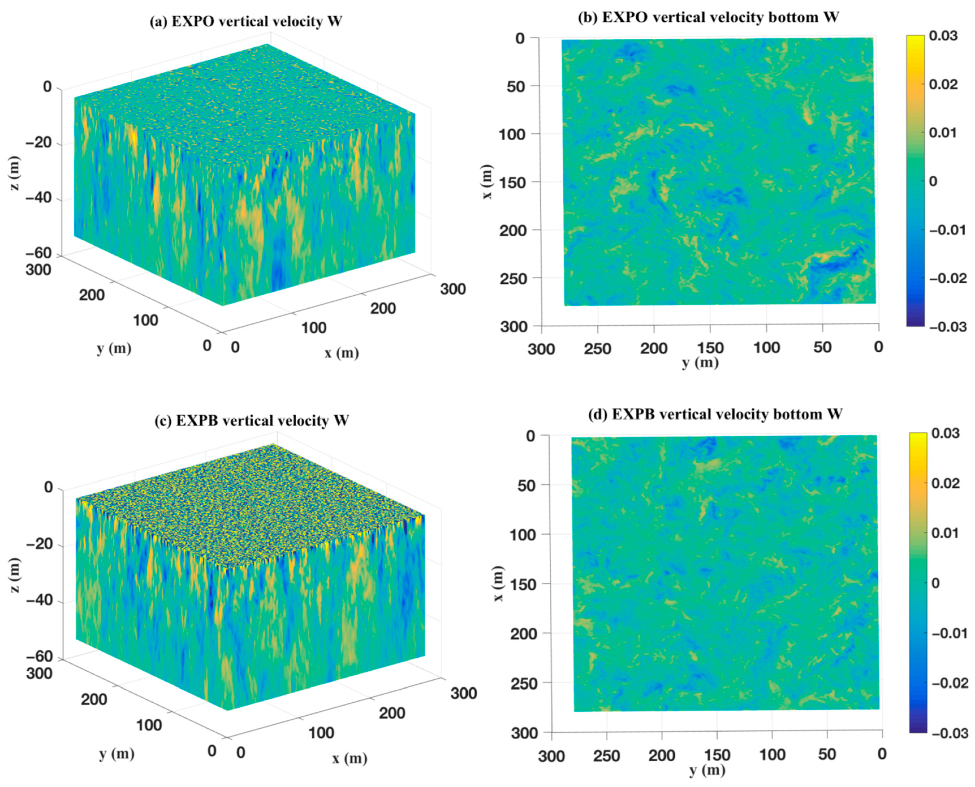
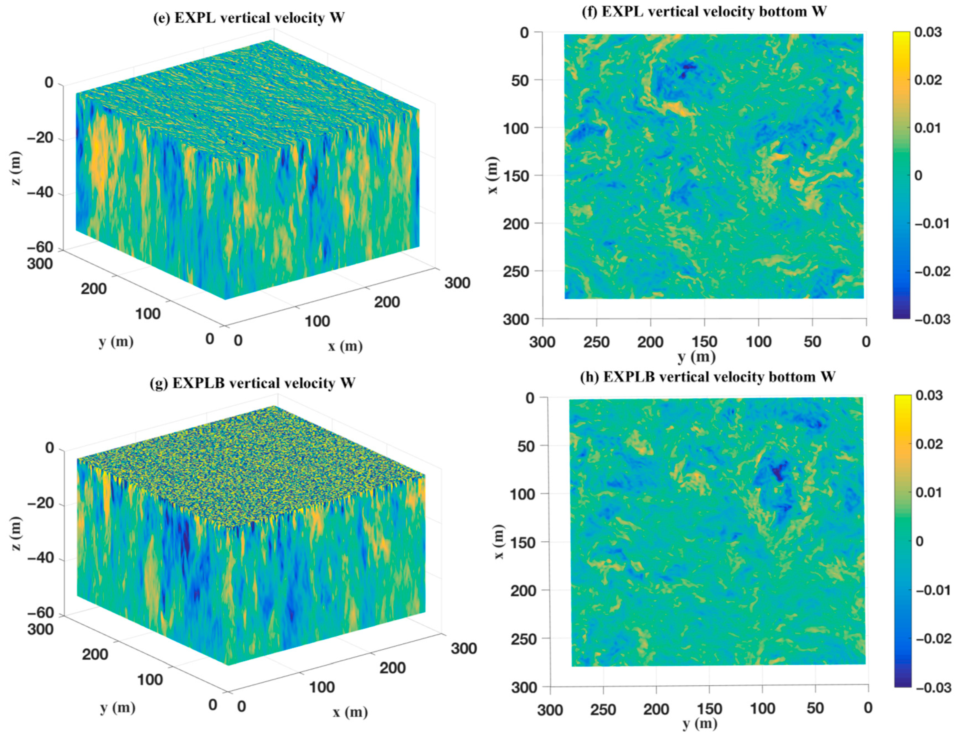
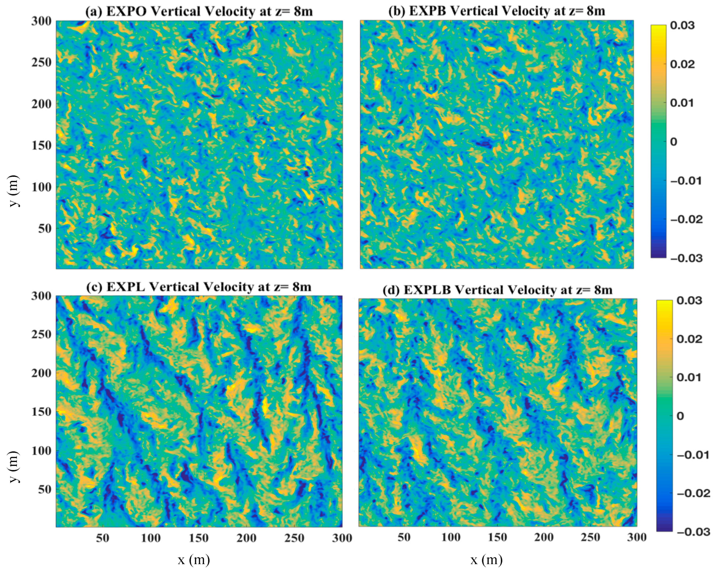
3.1. Vertical Velocity, Wavelength and Wave Height
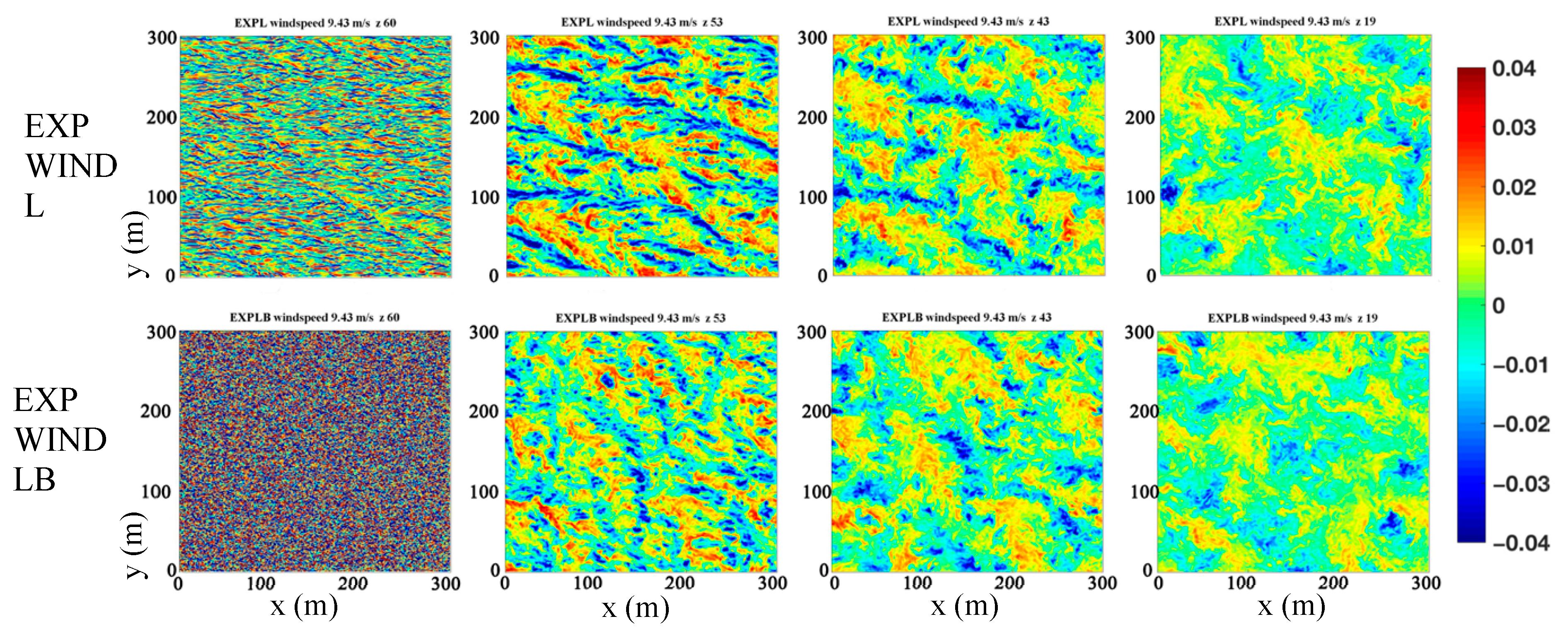
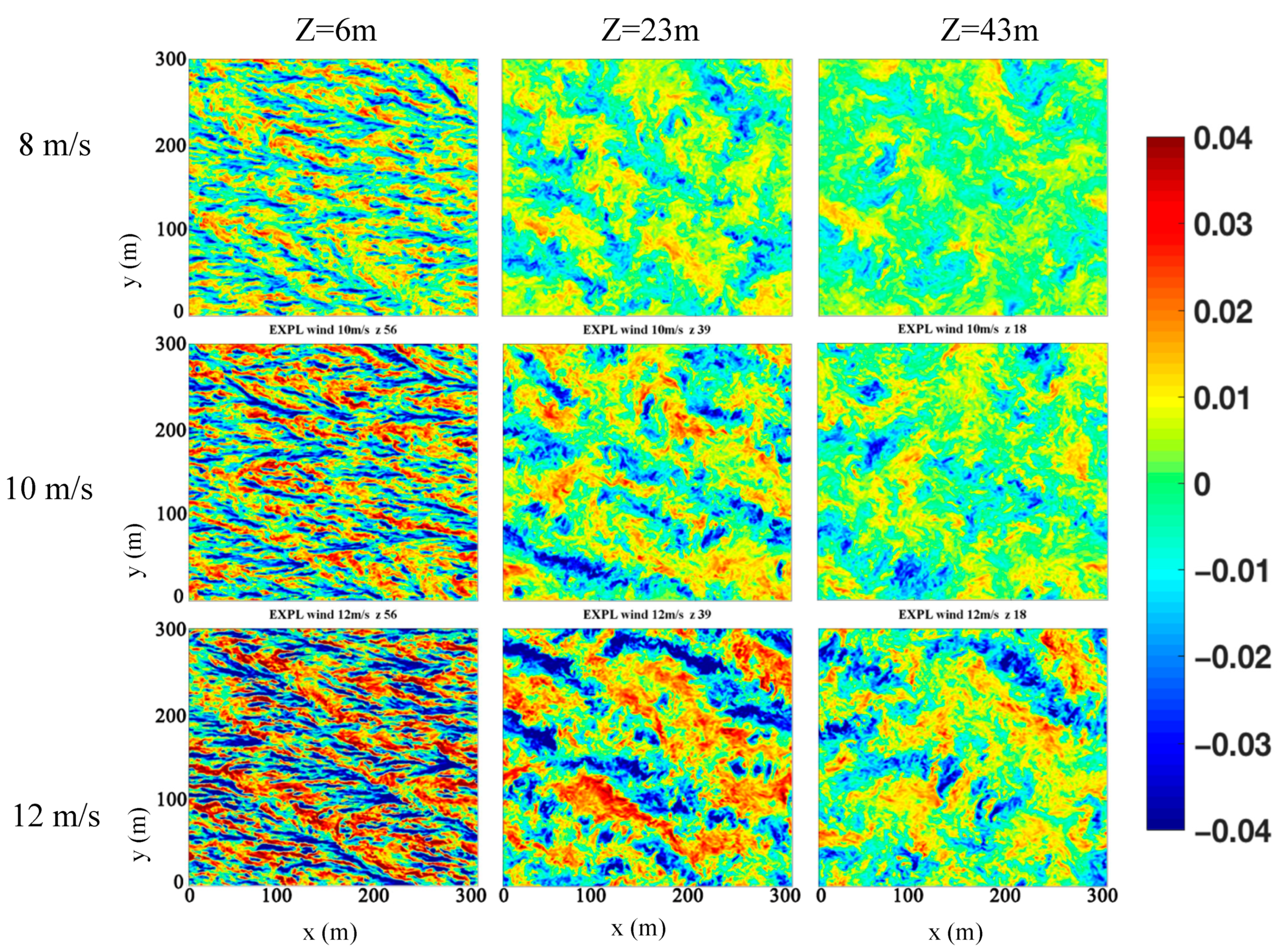
In order to analyze the influence of BW and LC on the mixed layer, vertical velocity is examined in this subsection with four experiments being performed. Experiment EXPO considered vertical velocity profiles without the influence of BW and LC, EXPB included only BW, EXPL included only LC, and EXPLB considered both LC and BW. The three-dimensional instantaneous vertical velocity fields (from the surface to a depth of 51 m) from the four experiments are plotted in Figure 1a (EXPO), c (EXPB), e (EXPL) and g (EXPLB), respectively. Corresponding vertical velocity fields at 51 m are plotted in Figure 1b (EXPO), d (EXPB), f (EXPL), h (EXPLB). The horizontal cross-sections (z = 8 m) of EXPO, EXPB, EXPL and EXPLB are plotted in Figure 2a–d, respectively.
From Figure 1c,g (EXPB and EXPLB, respectively), it can be observed that small-scale turbulence as generated by BW appeared only near the surface, enhancing the velocity field intensity. From Figure 1a–d, there were minimal differences between EXPB and EXPO. When BW was considered, strong small-scale turbulence was enhanced near the surface (Figure 1a,c). In Figure 2d, stripes, indicative of LC, could be observed below the near-surface, confirming that the influence of BW was limited to the near-surface. Downward velocity in EXPLB (Figure 2c) was slightly weaker than in EXPL (Figure 2d), demonstrating that BW may disturb the formation of Langmuir cells at the sea surface.
When LC was considered (EXPL and EXPLB), vertical velocity fields were significantly affected (Figure 1e,g). In the presence of LC (Figure 1e and Figure 2c,d), stripes were parallel to one another, indicating the formation of Langmuir cells. Moreover, the downwelling velocity field, which increased up to 0.03 m/s, was narrower and more intense than the upwelling velocity field. In Figure 1e and Figure 2c, the stripes widened, and their number decreased as depth increased. Furthermore, it can also be observed that the distance between stripes increased with depth.
From Figure 1f,h, the downwelling zone was fragmented and became dispersed, showing that the influence of LC was restricted by depth. The comparison of Figure 1b,d,f,h illustrates that the vertical velocity with LC was larger than that without LC. The value of vertical velocity was nearly unchanged when only considering BW (EXPB), which means the influence of BW was limited.
In summary, from the analysis of the above four experiments, it can be concluded that the inclusion of the LC generated stripes of strong vertical velocities down to a certain depth, the inclusion of the BW generated small-scale turbulence and weakened the near-surface LC, and the LC could influence ocean mixing to a greater depth than BW.
To test the sensitivity of wavelengths and wave heights on LC in the mixed layer, a series of wave conditions featured by varying wavelengths and wave heights were used to drive the LES model. In Figure 3, a horizontal cross-section of vertical velocity (z = 8 m) is displayed under different wavelengths and wave heights. The effects of LC and BW were included in all the experiments. Results show that when the wavelength was constant, the magnitude of the vertical velocity increased as wave height increased. Furthermore, it is observed that when wave heights increased, the Langmuir number decreased (Table 1) and the vertical velocity increased. The stripes became more evident and more coherent. Alternatively, when the wave height was constant, the Langmuir number increased as wavelength increased (Table 1), but the value of the vertical velocity remained almost unchanged. The above results suggest that LC was more sensitive to changes in wave heights rather than changes in wavelengths.

3.2. Wind Speed

However, although Equation (3) was used to calculate Stokes drift, and in the above experiments (see Figure 3), with different wavelengths and wave heights, was used to validate the effects that different monochromatic wave-generated LC has on upper-ocean mixed layer vertical velocity, the real ocean is polychromatic, rather than monochromatic. Consequently, Equation (5) was better at representing the effects LC had on wave-induced mixing. Using Equation (5), Figure 4 presents horizontal cross-sections of instantaneous vertical velocity fields from two new experiments (where EXP WIND L considered just LC and EXP WIND LB considered both LC and BW) with increasing depths (z = 1, 8, 18, and 42 m). It can be observed that stripes appeared in both experiments but the phenomenon was more apparent in EXP WIND L than in EXP WIND LB, especially near the sea surface. It can be highlighted that as compared to Figure 1c (EXPL), the instantaneous vertical velocity profiles of Figure 4 were stronger. When z = 42 m, the downwelling zone’s striping pattern could still be observed, suggesting that the depth of LC influence was deeper than in EXPL (Figure 1f). In the presence of LC, near-surface velocity fields exhibited striping patterns. In contrast, in the presence of BW (EXP WIND LB), near-surface velocity fields were dominated by small-scale turbulence and striping patterns appeared several meters below the surface. Comparing EXP WIND LB and EXP WIND L, it can be inferred that BW weakened LC. Leibovich [54] points out that when wind speeds were on the order of 8–18 m/s, phenomena such as turbulence and submesoscale processes may have intermittently occurred. Therefore, wind speeds from 8–16 m/s were chosen to investigate the response of the upper-ocean mixed layer to wind speeds under different Langmuir number settings (Table 2).
Three representative wind speeds were chosen: 8, 10 and 12 m/s (Figure 5). When the wind speed was 8 m/s, the vertical velocity decreased as depth increased. The stripes became less obvious, the distance between them got larger, and at 43 m depth, the stripes disappeared. When the wind speed was 10 m/s, the same phenomenon was observed as depth increased but stripes were still noticeable at 43 m. When the wind speed was 12 m/s, stripes also existed. They were more obvious than when the wind speed was less than 12 m/s. The vertical velocity increased as the wind speed increased. Stripe width increased with wind speeds. When the wind speed was 8 m/s, at z = 43 m, the velocity field was less isotropic. When the wind speed was 12 m/s, at z = 43 m, stripes could still be observed on the velocity field. Consequently, it can be surmised that different intensities of wind speed generated different LC. As wind speed increased, the influence depth of LC deepened.

3.3. Eddy Viscosity

The profile of mean eddy viscosity for momentum K m (Figure 6) is deduced from Equation (7), where ( u ¯ , v ¯ ) is the mean horizontal velocity. Eddy viscosity is usually used to quantify the upper ocean mixing strength and mixed layer depth as a mixing coefficient [55]. In both Figure 6a,b, we can see that Langmuir cells increased eddy viscosity, congruent with results from Noh et al. [56] which suggests that LC made the eddy viscosity K m much larger within the mixed layer. When considering LC (LB and L), the eddy viscosity of polychromatic waves (Figure 6b) was much larger than that of monochromatic waves (Figure 6a). The result of the picture suggests that BW could not, alone, change the eddy viscosity to a noticeable degree. However, only in conjunction with LC, could BW change eddy viscosity profiles and even decrease eddy viscosity. Moreover, LC together with BW could influence ocean mixing strength and mixed layer depth.
u w ¯ u ¯ / z v w ¯ v ¯ / z = K m [ ( u ¯ / z ) 2 + ( v ¯ / z ) 2 ]

4. Discussion and Conclusions

As previously highlighted, most traditional turbulence models do not consider the effects of LC and BW in their simulations. Furthermore, as model resolutions increase, existing parameterizations need to be more refined. Consequently, in our research, the LC and BW are added to the large eddy simulation to examine the wave-induced mixing and its parameterization. Six kinds of experiments are carried out so that the effects of BW and LC could be examined singularly, in addition to their joint effects. Through these experiments, it is found that:
(1)
The presence of LC could generate stripes of strong vertical velocities to a certain depth, BW could produce small-scale turbulences on the sea surface and could weaken LC near the surface, and LC can influence the mixing to a greater depth than BW. Therefore, it is proposed that the vortex force is a much more effective mechanism in deepening the mixed layer than BW.
(2)
It is also identified that as wave heights increase, stripes become more evident. When wavelengths increase, by contrast, vertical velocities are not modified significantly, thus suggesting that the wave-induced mixing is more sensitive to the wave height than to the wavelength.
(3)
The Stokes drift velocity and the vertical velocity increase with the wind speed with stripes becoming more evident as well. The influence of LC increases with wind speed.
(4)
With increasing depth, the number of stripes declines and stripes become more coherent.
(5)
Model results and calculations indicate that LC increases eddy viscosity within the mixed layer, in accordance with previous findings [56]. Additionally, although it is identified that BW could not influence eddy viscosity alone, BW working in tandem with LC leads to reductions in eddy viscosity. The eddy viscosity of polychromatic waves is larger than that of monochromatic waves. Wave-induced mixing could influence the eddy viscosity and enhance the mixing efficiency.
Based on the above conclusions, it is estimated that a mean eddy viscosity assumption in the presence of Langmuir cells is not enough. The wave-induced mixing should be considered in the eddy viscosity assumption. A new parametric relationship in the upper layer should be derived to describe this phenomenon more accurately. As only a few studies which cover this topic exist [55], parameterized results still contain errors. This problem will be addressed in a future publication in which a new parameterization which relates to the Langmuir number, the Stokes drift and the mixed layer depth will be derived. Stratification in the mixing layer and the application of the new parameterization will also be analyzed.

Author Contributions

Methodology, H.W. and C.D.; software, H.W. and X.G.; formal analysis, H.W. and C.D. and Y.Y. All authors have read and agreed to the published version of the manuscript.

Funding

This research was funded by the National Key Research and Development Program of China (2017YFA0604100, 2016YFA0601803, and 2016YFC1401407), the National Natural Science Foundation of China (41476022, 41490643, and 41706008), the National Programme on Global Change and Air–Sea Interaction (GASI-IPOVAI-02, GASI-03-IPOVAI-05), and the China Ocean Mineral Resources R&D Association (DY135-E2-2-02, DY135-E2-3-01).

Acknowledgments

This work was supported by the China Scholarship Council (CSC) scholarship. Thanks are also extended to Baylor Fox-Kemper for his advice in conducting this research.

Conflicts of Interest

The authors declare no conflict of interest. The funders had no role in the design of the study; in the collection, analyses, or interpretation of data; in the writing of the manuscript, or in the decision to publish the results.

References

  1. Kantha, L.H.; Clayson, C.A. On the effect of surface gravity waves on mixing in the oceanic mixed layer. Ocean. Model 2004, 6, 101–124. [Google Scholar] [CrossRef]
  2. Craik, A.D.D.; Leibovich, S. A rational model for Langmuir circulations. J. Fluid Mech. 1976, 73, 401–426. [Google Scholar] [CrossRef] [Green Version]
  3. Leibovich, S. The form and Dynamics of Langmuir Circulations. Ann. Rev. Fluid Mech. 1983, 15, 391–427. [Google Scholar] [CrossRef] [Green Version]
  4. Smith, J.A. Observations and Theories of Langmuir Circulation: A Story of Mixing Fluid Mechanics and the Environment: Dynamical Approaches; Lumely, J., Ed.; Springer: New York, NY, USA, 2001; pp. 295–314. [Google Scholar]
  5. Thorpe, S.A. Langmuir circulation. Annu. Rev. Fluid Mech. 2004, 36, 55–79. [Google Scholar] [CrossRef]
  6. Mcwilliams, J.C.; Sullivan, P.; Moeng, C. Langmuir turbulence in the ocean. J. Fluid Mech. 1997, 334, 1–30. [Google Scholar] [CrossRef] [Green Version]
  7. Noh, Y.; Min, H.S.; Raasch, S. Large Eddy Simulation of the Ocean Mixed Layer: The Effects of Wave Breaking and Langmuir Circulation. J. Phys. Oceanogr. 2004, 34, 720–735. [Google Scholar] [CrossRef]
  8. Li, M.; Garrett, C.; Skyllingstad, E. A regime diagram for classifying turbulent large eddies in the upper ocean. Deep-Sea. Res. Pt. I. 2005, 52, 259–278. [Google Scholar] [CrossRef]
  9. Skyllingstad, E.D. Langmuir Circulation. Marine Turbulence; Baumert, H.Z., Simpson, J.H., Sündermann, J., Eds.; Cambridge University Press: Cambridge, UK, 2005; pp. 277–282. [Google Scholar]
  10. Harcourt, R.R.; D’Asaro, E.A. Large-eddy simulation of Langmuir turbulence in pure wind seas. J. Phys. Oceanogr. 2008, 38, 1542–1562. [Google Scholar] [CrossRef]
  11. Grant, A.L.M.; Belcher, S.E. Characteristics of langmuir turbulence in the ocean mixed layer. J. Phys. Oceanogr. 2009, 39, 1871–1887. [Google Scholar] [CrossRef] [Green Version]
  12. Melville, W.K. The role of surface-wave breaking in air–sea interaction. Annu. Rev. Fluid Mech. 1996, 28, 279–321. [Google Scholar] [CrossRef]
  13. Terray, E.; Donelan, M.; Agrawal, Y.; Drennan, W.M.; Kahma, K.K.; Williams, A.J.; Hwang, P.A.; Kitaigorodskii, S.A. Estimates of kinetic energy dissipation under breaking waves. J. Phys. Oceanogr. 1996, 26, 792–807. [Google Scholar] [CrossRef] [Green Version]
  14. Craig, P.D.; Banner, M.L. Modeling wave-enhanced turbulence in the ocean surface layer. J. Phys. Oceanogr. 1994, 24, 2546–2559. [Google Scholar] [CrossRef] [Green Version]
  15. Mellor, G.L.; Yamada, T. Development of a turbulent closure model for geophysical fluid problems. Rev. Geophys. Space Phys. 1982, 20, 851–875. [Google Scholar] [CrossRef] [Green Version]
  16. Large, W.G.; McWilliams, J.C.; Doney, S.C. Oceanic vertical mixing: A review and a model with a nonlocal boundary layer parameterization. Rev. Geophys. 1994, 32, 363–403. [Google Scholar] [CrossRef] [Green Version]
  17. Li, X.; Chao, Y.; Mcwilliams, J.C.; Fu, L.L. A Comparison of Two Vertical-Mixing Schemes in a Pacific Ocean General Circulation Model. J. Clim. 2001, 14, 1377–1398. [Google Scholar] [CrossRef] [Green Version]
  18. Kara, A.B.; Wallcraft, A.J.; Hurlburt, H.E. Climatological SST and MLD Predictions from a Global Layered Ocean Model with an Embedded Mixed Layer. J. Atmos. Ocean. Tech. 2003, 20, 1616–1632. [Google Scholar] [CrossRef] [Green Version]
  19. Gnanadesikan, A.; Dixon, K.W.; Griffies, S.M. GFDL’s CM2 Global Coupled Climate Models. Part II: The Baseline Ocean Simulation. J. Clim. 2006, 19, 675–697. [Google Scholar] [CrossRef]
  20. Fox-Kemper, B.; Danabasoglu, G.; Ferrari, R. Parameterization of mixed layer eddies. III: Implementation and impact in global ocean climate simulations. Ocean Model. 2011, 39, 61–78. [Google Scholar] [CrossRef] [Green Version]
  21. Belcher, E.; Grant, M.; Hanley, E. A global perspective on Langmuir turbulence in the ocean surface boundary layer. Geophys. Res. Lett. 2012, 39, 9. [Google Scholar] [CrossRef] [Green Version]
  22. Schiller, A.; Ridgway, K.R. Seasonal mixed-layer dynamics in an eddy-resolving ocean circulation model. J. Geophys. Res-Oceans. 2013, 118, 3387–3405. [Google Scholar] [CrossRef]
  23. Halpern, D.; Chao, Y.; Ma, C.C. Comparison of tropical pacific temperature and current simulations with two vertical mixing schemes embedded in an ocean general circulation model and reference to observations. J. Geophys. Res-Oceans. 1995, 100, 2515–2522. [Google Scholar] [CrossRef]
  24. Large, W.G.; Danabasoglu, G. Attribution and Impacts of Upper-Ocean Biases in CCSM3. J. Clim. 2006, 19, 2325–2346. [Google Scholar] [CrossRef] [Green Version]
  25. Tsujino, H.; Hirabara, M.; Nakano, H.; Yasuda, T.; Motoi, T.; Yamanaka, G. Simulating present climate of the global ocean–ice system using the Meteorological Research Institute Community Ocean Model (MRI.COM): Simulation characteristics and variability in the Pacific sector. J. Oceanogr. 2011, 67, 449–479. [Google Scholar] [CrossRef]
  26. Noh, Y.; Ok, H.; Lee, E.; Toyoda, T.; Hirose, N. Parameterization of Langmuir Circulation in the Ocean Mixed Layer Model Using LES and its Application to the OGCM. J. Phys. Oceanogr. 2015, 46, 57–58. [Google Scholar] [CrossRef]
  27. Meehl, G.A.; Gent, P.R.; Arblaster, J.M.B.; Otto-Bliesner, L.; Brady, E.C.; Craig, A. Factors that affect the amplitude of El Niño in global coupled climate models. Clim. Dyn. 2001, 17, 515–526. [Google Scholar] [CrossRef]
  28. Pacanowski, R.C.; Philander, S.G. Parameterization of Vertical Mixing in Numerical Models of the Tropical Oceans. J. Phys. Oceanogr. 1981, 11, 1443–1451. [Google Scholar] [CrossRef]
  29. Rosati, A.; Miyakoda, K. A General Circulation Model for Upper Ocean Simulation. J. Phys. Oceanogr. 1988, 18, 1601–1626. [Google Scholar] [CrossRef]
  30. Blanke, B.; Delecluse, P. Variability of the Tropical Atlantic Ocean Simulated by a General Circulation Model with Two Different Mixed-Layer Physics. J. Phys. Oceanogr. 1993, 23, 1363–1388. [Google Scholar] [CrossRef] [Green Version]
  31. Chen, D.; Rothstein, L.M.; Busalacchi, A.J. A Hybrid Vertical Mixing Scheme and Its Application to Tropical Ocean Models. J. Phys. Oceanogr. 1994, 24, 2156–2179. [Google Scholar] [CrossRef] [Green Version]
  32. Sterl, A.; Kattenberg, A. Embedding a mixed layer model into an ocean general circulation model of the Atlantic: The importance of surface mixing for heat flux and temperature. J. Geophys. Res-Oceans. 1994, 99, 14139–14157. [Google Scholar] [CrossRef]
  33. Large, W.G.; Danabasoglu, G.; Doney, S.C.; McWilliams, J.C. Sensitivity to Surface Forcing and Boundary Layer Mixing in a Global Ocean Model: Annual-Mean Climatology. J. Phys. Oceanogr. 1997, 27, 2418–2447. [Google Scholar] [CrossRef]
  34. Burchard, H.; Bolding, K. Comparative analysis of four second moment turbulence closure models for the ocean mixed layer. J. Phys. Oceanogr. 2001, 31, 1943–1968. [Google Scholar] [CrossRef]
  35. Noh, Y.; Jang, C.J.; Yamagata, T. Simulation of More Realistic Upper-Ocean Processes from an OGCM with a New Ocean Mixed Layer Model. J. Phys. Oceanogr. 2002, 32, 1284–1307. [Google Scholar] [CrossRef] [Green Version]
  36. Qiao, F.L.; Yuan, Y.L.; Yang, Y.Z.; Zheng, Q.; Xia, C.; Ma, J. Wave-induced mixing in the upper ocean:Distribution and application in a global ocean circulation model. Geophys. Res. Lett. 2004, 31, L11303. [Google Scholar] [CrossRef]
  37. Fox-Kemper, B.; Ferrari, R.; Hallberg, R.W. Parameterization of mixed layer eddies. Part I: Theory and diagnosis. J. Phys. Oceanogr. 2008, 38, 1145–1165. [Google Scholar] [CrossRef]
  38. Richards, K.J.; Xie, S.P.; Miyama, T. Vertical mixing in the ocean and its impact on the coupled ocean/atmosphere system in the Eastern Tropical Pacific. J. Clim. 2009, 22, 3703–3719. [Google Scholar] [CrossRef]
  39. Sasaki, W.; Richards, K.J.; Luo, J.J. Role of vertical mixing originating from small vertical scale structures within the equatorial thermocline in an OGCM. Ocean Model. 2012, 57, 29–42. [Google Scholar] [CrossRef]
  40. Li, Y.; Qiao, F.; Yin, X.; Shu, Q.; Ma, H. The improvement of the one-dimensional Mellor-Yamada and K-profile parameterization turbulence schemes with the non-breaking surface wave-induced vertical mixing. Acta Oceanol. Sin. 2013, 32, 62–73. [Google Scholar] [CrossRef]
  41. Skyllingstad, E.D.; Denbo, D.W. An ocean large-eddy simulation of Langmuir circulations and convection in the surface mixed layer. J. Geophys. Res. 1995, 100, 8501–8522. [Google Scholar] [CrossRef]
  42. Sullivan, P.P.; Mcwilliams, J.C.; Kendall, M.W. Surface gravity wave effects in the oceanic boundary layer: Large-eddy simulation with vortex force and stochastic breakers. J. Fluid. Mech. 2007, 593, 405–452. [Google Scholar] [CrossRef] [Green Version]
  43. Mcwilliams, J.C.; Huckle, E.; Liang, J.H.; Sullivan, P.P. The Wavy Ekman Layer: Langmuir Circulations, Breaking Waves, and Reynolds Stress. J. Phy. Oceanogr. 2012, 42, 1793–1816. [Google Scholar] [CrossRef]
  44. Sullivan, P.P.; Romero, L.; Mcwilliams, J.C.; Melville, W.K. Transient evolution of Langmuir turbulence in ocean boundary layers driven by hurricane winds and waves. J. Phys. Oceanogr. 2012, 42, 1959–1980. [Google Scholar] [CrossRef]
  45. Skyllingstad, E.D.; Crawford, G.B. Resonant wind-driven mixing in the ocean boundary layer. J. Phys. Oceanogr. 2000, 30, 219–237. [Google Scholar] [CrossRef]
  46. Sanford, T.B.; Price, J.F.; Girton, J.B.; Webb, D.C. Upper-ocean response to Hurricane Frances (2004) observed by profiling EM-Apex floats. J. Phys. Oceanogr. 2011, 41, 1041–1056. [Google Scholar] [CrossRef]
  47. Kukulka, T.; Brunner, K. Passive buoyant tracers in the ocean surface boundary layer: 1. Influence of equilibrium wind-waves on vertical distributions. J. Geophys. Res-Oceans. 2015, 120, 3837–3858. [Google Scholar] [CrossRef]
  48. Brunner, K.; Kukulka, T.; Proskurowski, G. Passive buoyant tracers in the ocean surface boundary layer: 2. Observations and simulations of microplastic marine debris. J. Geophys. Res-Oceans. 2016, 120, 7559–7573. [Google Scholar] [CrossRef] [Green Version]
  49. Maronga, B.; Gryschka, M.; Heinze, R.; Hoffmann, F.; Kanani-Sühring, F.; Keck, M.; Ketelsen, K.; Letzel, M.O.; Sühring, M.; Raasch, S. The Parallelized Large-Eddy Simulation Model (PALM) version 4.0, for atmospheric and oceanic flows: Model formulation, recent, developments, and future perspectives. Geosci. Model Dev. 2015, 8, 2515–2551. [Google Scholar] [CrossRef] [Green Version]
  50. Briggs, D.A.; Ferziger, J.H.; Koseff, J.R.; Monismith, S.G. Entrainment in a shear-free turbulent mixing layer. J. Fluid Mech. 1996, 310, 215–241. [Google Scholar] [CrossRef]
  51. Smith, J.A. Observed growth of Langmuir circulation. J. Geophys. Res-Oceans. 1992, 97, 5651–5664. [Google Scholar] [CrossRef] [Green Version]
  52. Mcwilliams, J.C.; Restrepo, J.M. The Wave-Driven Ocean Circulation. J. Phy. Oceanogr. 1999, 29, 2523–2540. [Google Scholar] [CrossRef]
  53. Large, W.G.; Pond, S. Sensible and Latent Heat Flux Measurements over the Ocean. J. Phy. Oceanogr. 1982, 12, 464–482. [Google Scholar] [CrossRef] [Green Version]
  54. Leibovich, S. Reference Module in Earth Systems and Environmental Sciences. Langmuir Circulation and Instability. Encyclopedia of Ocean Sciences, 3rd ed.; Elsevier: Amsterdam, The Netherlands, 2009; pp. 1453–1461. [Google Scholar]
  55. Mcwilliams, J.C. Surface wave effects on submesoscale fronts and filaments. J. Fluid Mech. 2018, 843, 479–517. [Google Scholar] [CrossRef]
  56. Noh, Y.; Goh, G.; Raasch, S.; Gryschka, M. Influence of Langmuir Circulation on the Deepening of the Wind-Mixed Layer. J. Phys. Oceanogr. 2011, 41, 472–484. [Google Scholar] [CrossRef]
Figure 1. Distributions of three-dimensional vertical velocity (m/s) without Langmuir circulation (LC) and breaking waves (BW) (a); with only BW (c); with only LC (e) and with LC and BW (g). Horizontal cross-section of vertical velocity (z = 51 m) without LC and BW (b); with BW (d); with LC (f); with LC and BW (h).
Atmosphere 11 00207 g001aAtmosphere 11 00207 g001b
Figure 2. Horizontal cross-section of vertical velocity (m/s) (z = 8 m) without LC and BW (a); with only BW (b), with only LC (c); with LC and BW (d).
Atmosphere 11 00207 g002
Figure 3. Horizontal cross-section of vertical velocity (m/s) (z = 8 m). The EXPLB with different values of L a t ( L a t = 0.30, 0.26, 0.23, 0.37, 0.32, 0.29, 0.44, 0.38, 0.34).
Atmosphere 11 00207 g003
Figure 4. Horizontal cross-section of vertical velocity (m/s) (z = 1, 8, 18, and 42 m) for EXP WIND L and EXP WIND LB.
Atmosphere 11 00207 g004
Figure 5. Horizontal cross-section of vertical velocity (m/s) at 6 m (z56), 23 m (z39) and 43 m (z18) for EXP WIND L under different wind speed conditions (U = 8, 10 and 12 m/s).
Atmosphere 11 00207 g005
Figure 6. Vertical profile of the eddy viscosity K m for simulations with no BW and LC (blue); BW only (green); LC only (black); with LC and BW (red). Eddy viscosity is based on Stokes velocities calculated using Equation (3) (a) and Equation (5) (b).
Atmosphere 11 00207 g006
Table 1. Values of (turbulent Langmuir number) L a t for different combinations of wavelengths (λ, m) and wave heights (H, m).
H0.511.522.53.0
λ = 300.520.360.300.260.230.21
λ = 400.640.450.370.320.290.26
λ = 500.760.540.440.380.340.31
Table 2. Values of wind stress ( τ , N/m2) and turbulent Langmuir number (Lat) for different wind speeds (U, m/s).
τ ULat
0.0780.16
0.109.430.16
0.11100.16
0.15110.17
0.18120.17
0.23130.17
0.27140.17
0.33150.17
0.39160.18

