A Boundary Forcing Sensitivity Analysis of the West African Monsoon Simulated by the Modèle Atmosphérique Régional


Abstract
1. Introduction
1.1. General Context
1.2. Large-Scale Dynamics Biases Versus Regional-Scale Physical Errors
1.3. A Surrogate Approach for Assessing a Regional Model Sensitivity to Boundary Forcing Fields Errors
2. Materials and Methods
2.1. Model Description
2.2. Experimental Protocol
2.2.1. Domain and Input Data
2.2.2. Study Period
2.2.3. Protocol
- T00: control simulation
- T10: air temperature increase of 1 C over the whole atmospheric column,
- T01: horizontally homogeneous SST increase of 1 C,
- T11: a combination of the two previous perturbations.
3. Results
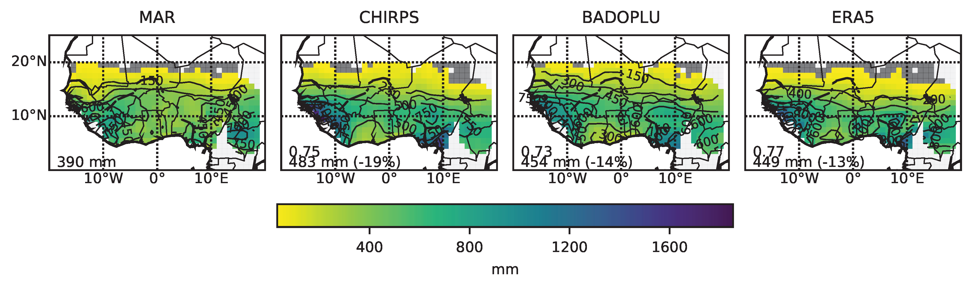
3.1. Model Evaluation
- CHIRPS [61], an observationally constrained satellite product available since 1982 covering the study period,
- BADOPLU (BAse de DOnnées PLUviomètres), a rain-gauge product gathering since 1950 in-situ observations from various national meteorological agencies in a fully quality-controlled dataset (see the supplementary materials of Panthou et al. [24] for a detailed description of the data processing). The point rainfall data from BADOPLU are spatially interpolated on a 1 × 1 regular grid by a block-kriging technique using a double exponential structure variogram (see [62] for details of the interpolation),
- ERA5 [63], the new global atmospheric reanalysis produced by the ECMWF, spanning the period from 1979 to present with a 0.25 × 0.25 grid spacing. Note that since ERA5 data were collected for a domain extending from 20 W–20 E and 0–20 N (from the Copernicus Climate Change Service portal: Https://Cds.Climate.Copernicus.Eu/Cdsapp#!/Home), this reduced window is considered for the model evaluation.
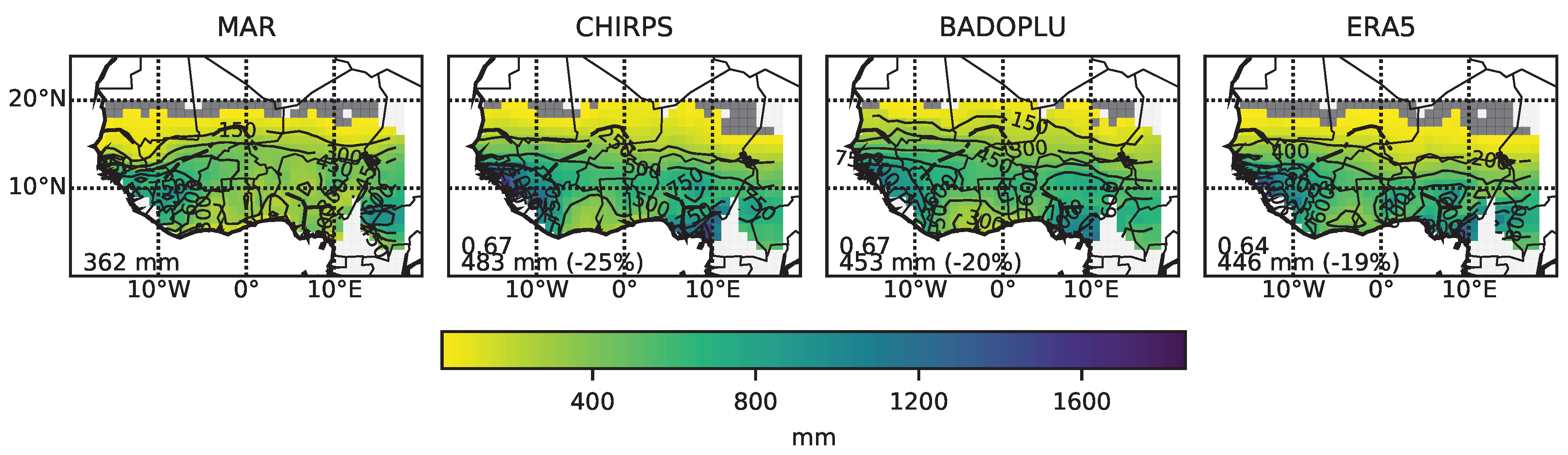
3.1.1. Spatial Pattern
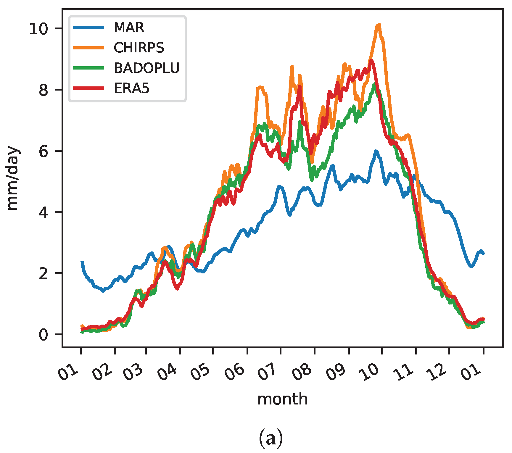
3.1.2. Seasonal Cycle
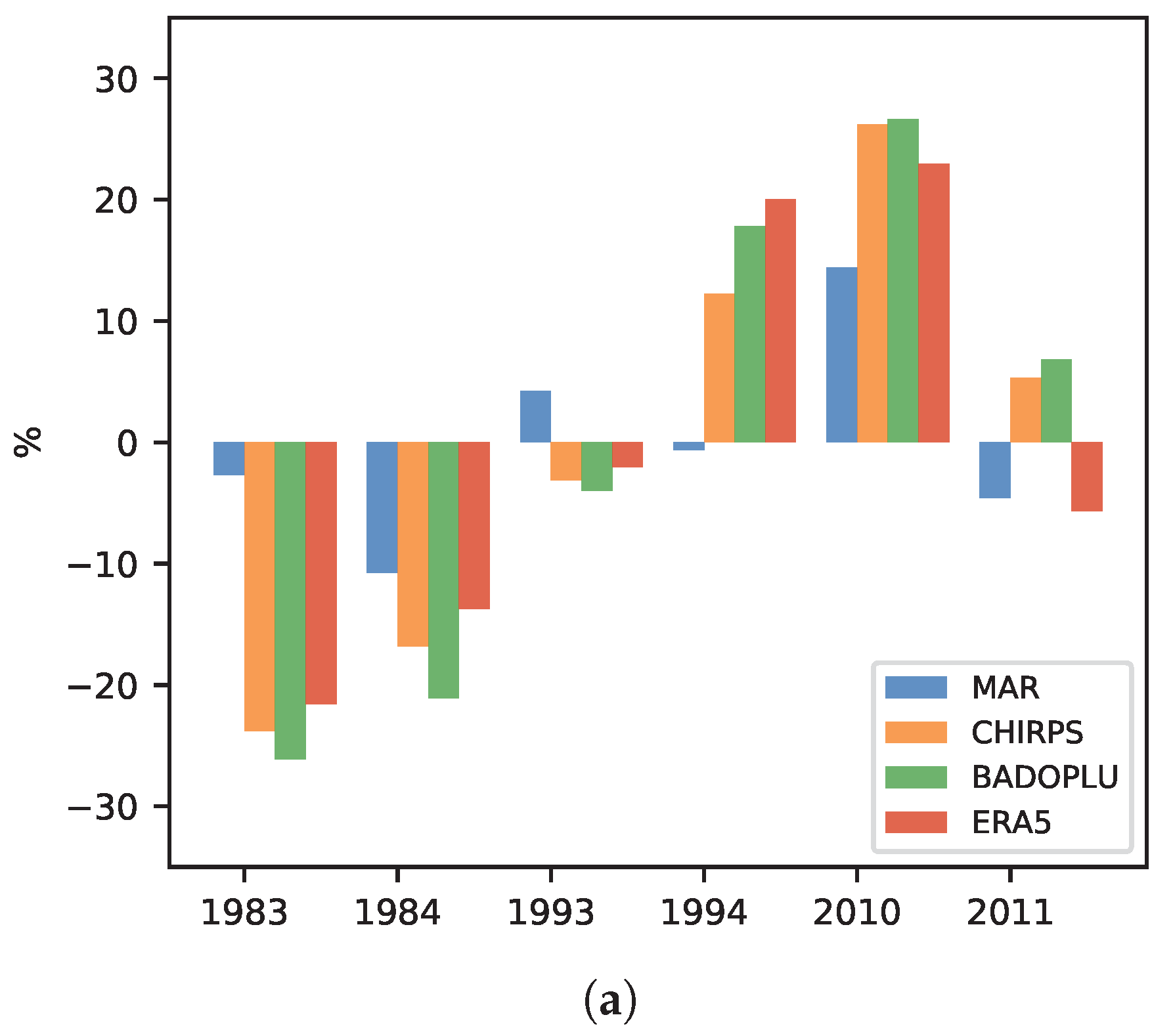
3.1.3. Interannual Variability
3.2. Sensitivity Experiment Results
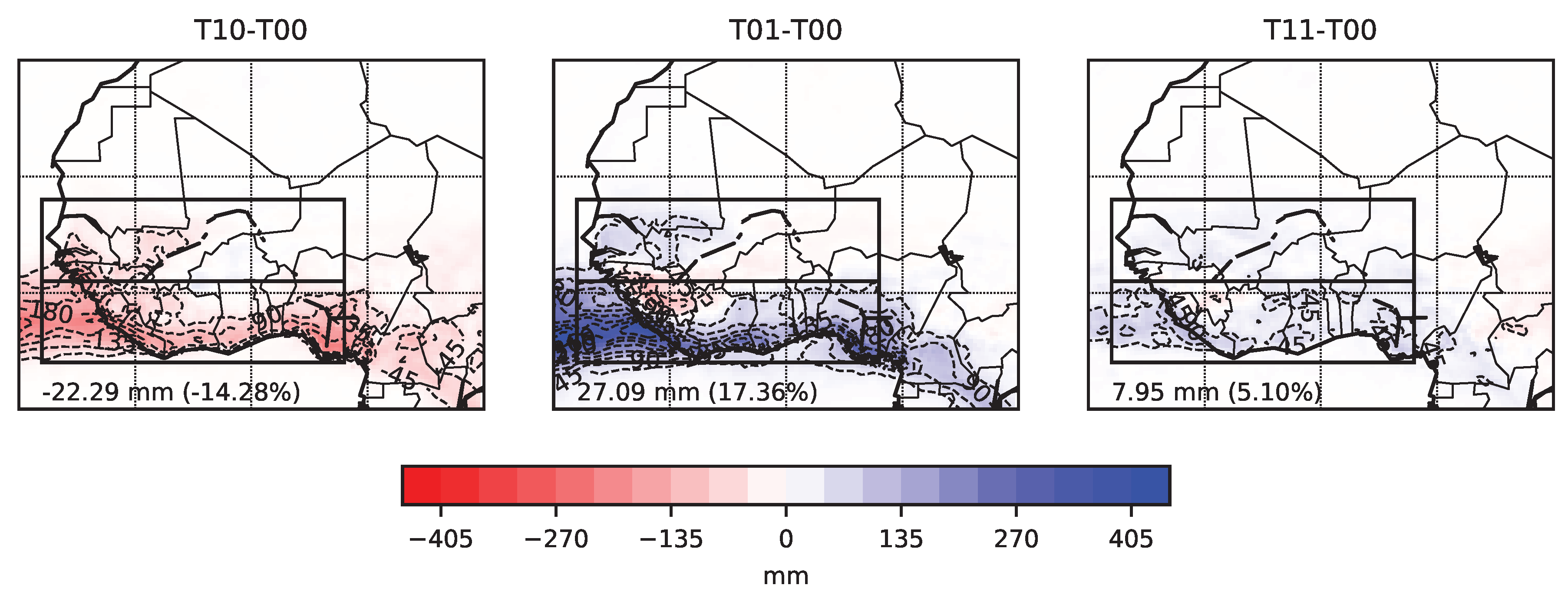
3.2.1. Rainfall Response
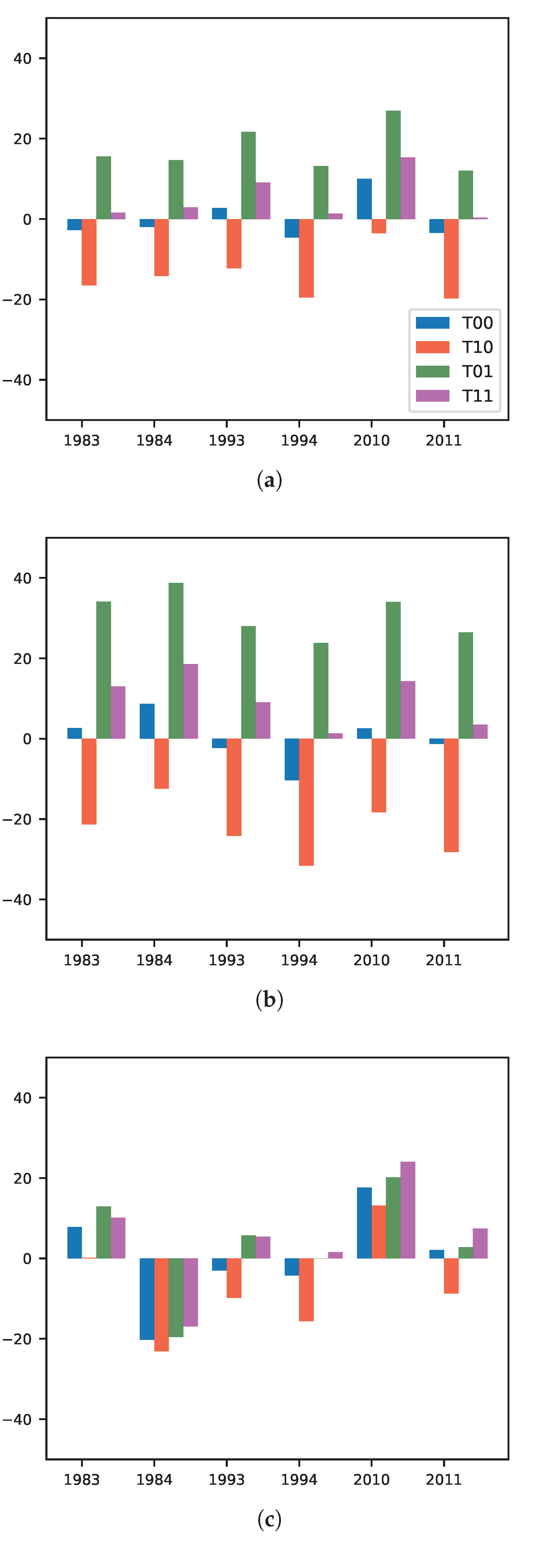
- the rainfall response to the perturbed boundary forcing over the regions of interest is unequivocal, with T10 on the one side and T01 and T11 on the other side always displaying dry and wet anomalies, respectively,
- over the WA domain and the Guinea region, the JAS rainfall changes are beyond the range of natural variability, defined by the interannual variability in the control simulation (blue bars in Figure 6). This feature indicates the strong model sensitivity to thermodynamical perturbations over this region and is suggestive of a dominant mechanism shaping the rainfall response. Over the Sahel, the rainfall anomalies relative to the study period average have the same amplitude as the control simulation interannual variability. Therefore, the dynamical influence (i.e., the year-to-year internal variability) on the boundary perturbation sensitivity may be larger in this region than over Guinea. Note here the added value of the sampled years, representative of distinct climatic conditions in West Africa, adding robustness to these conclusions.
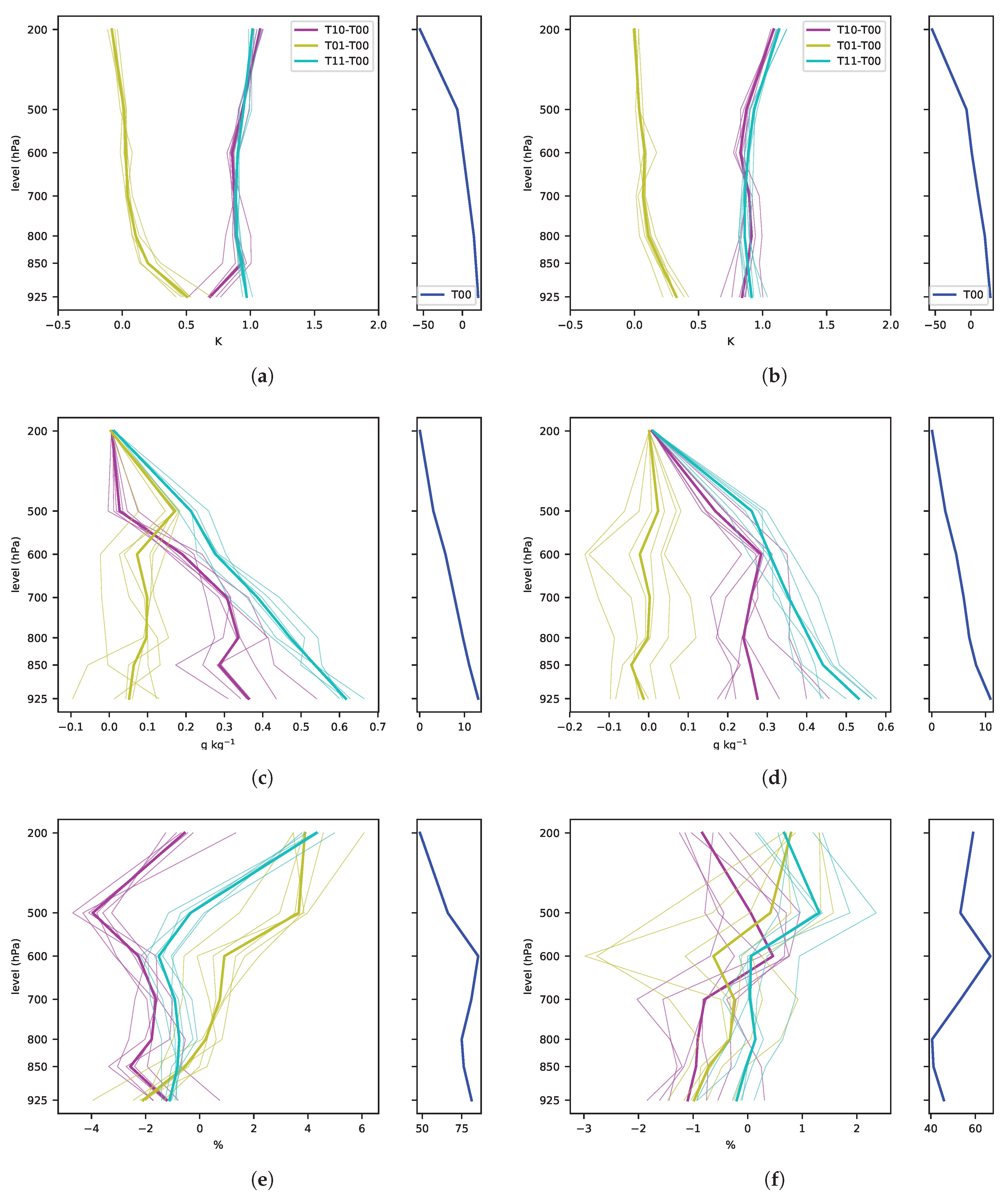
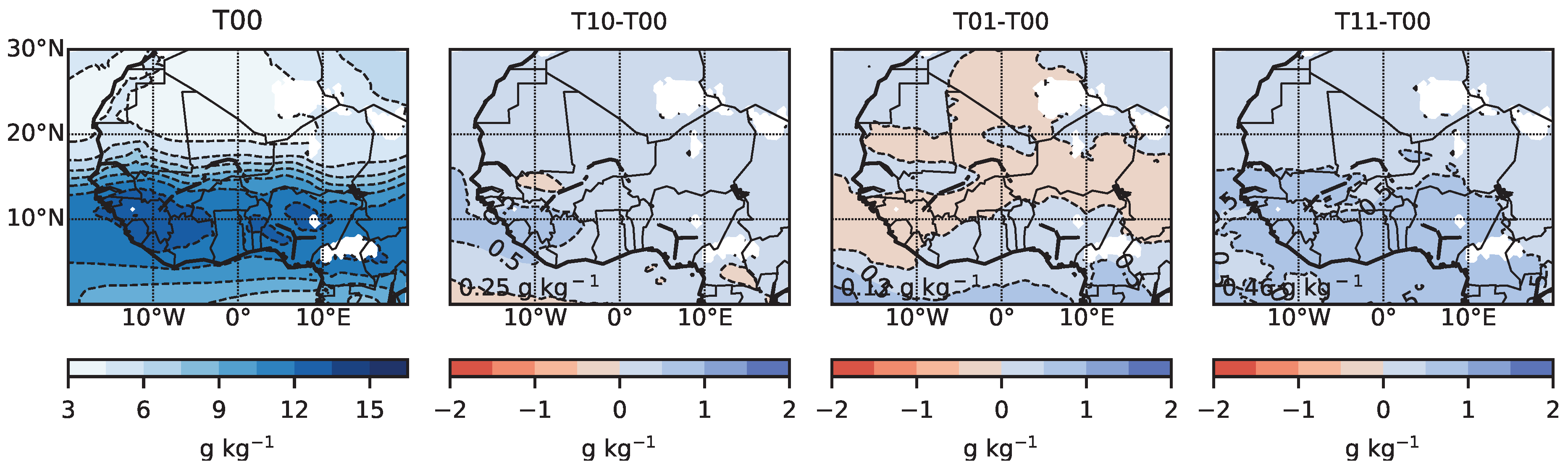
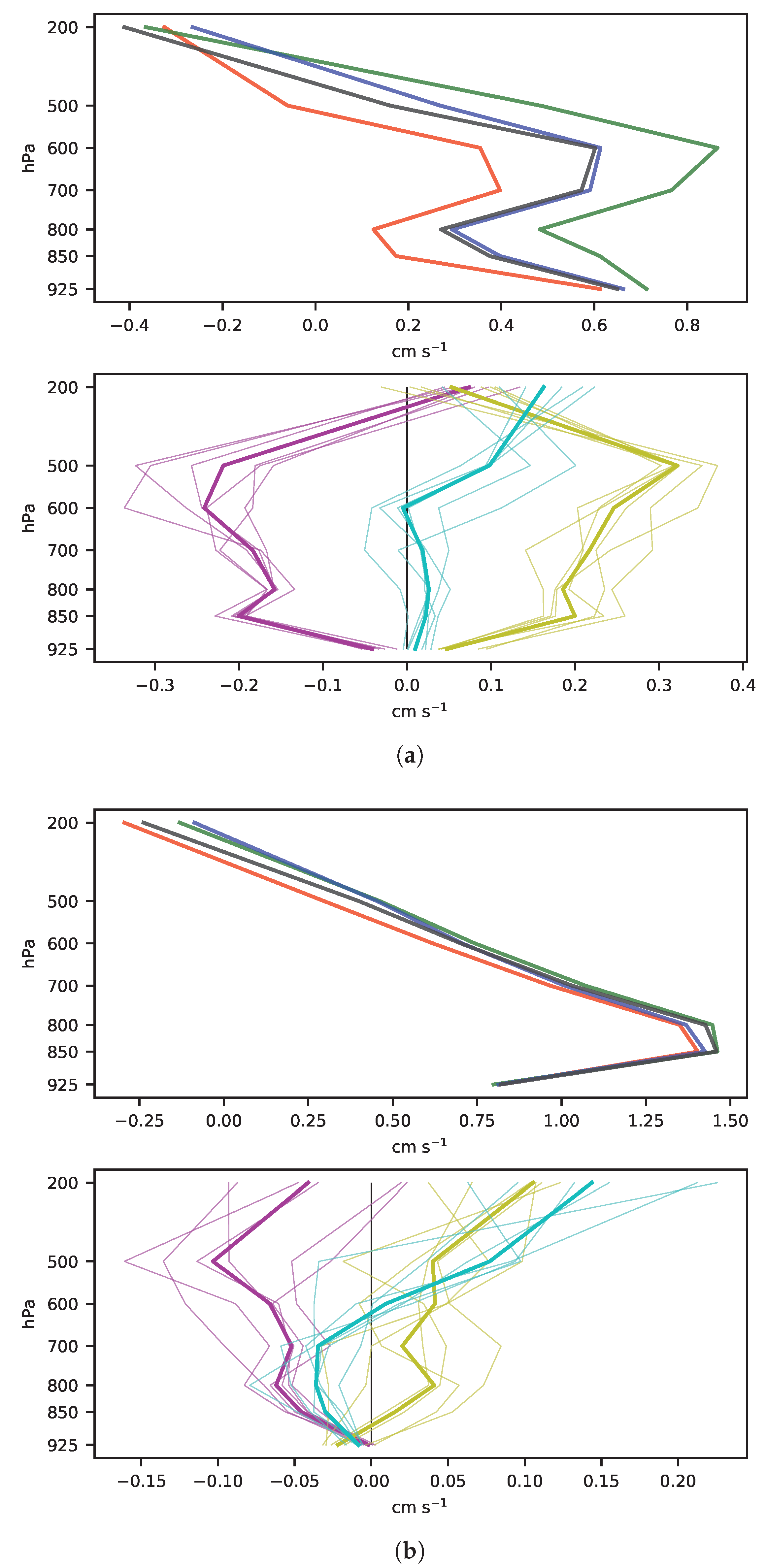
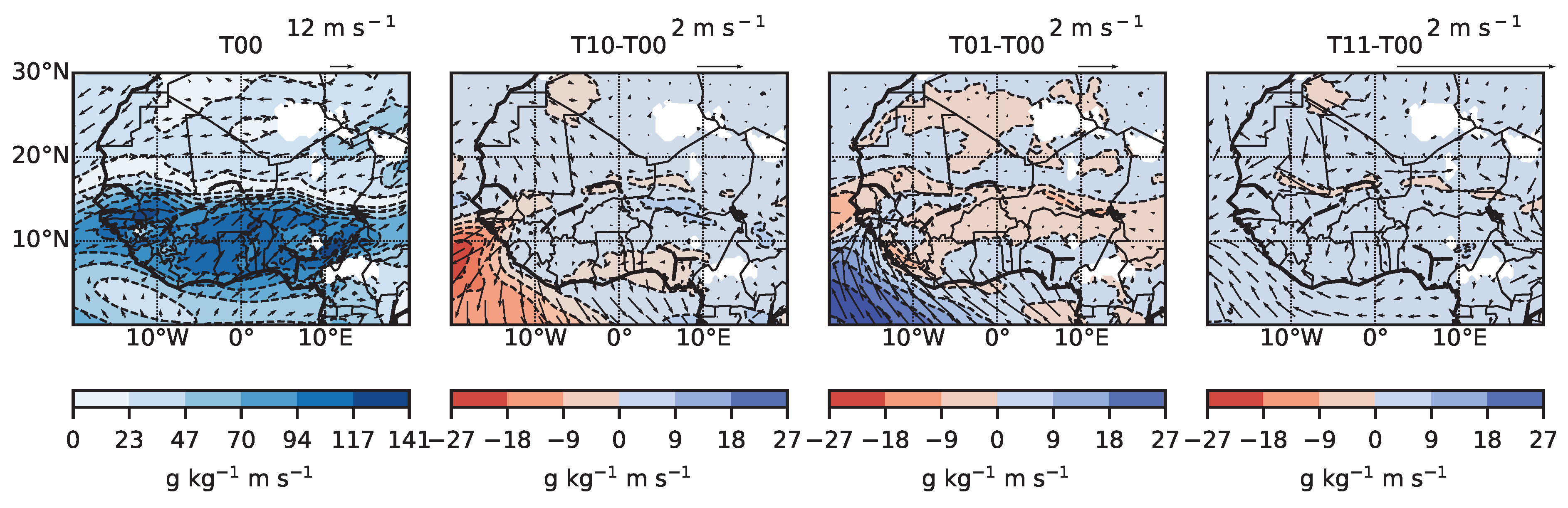
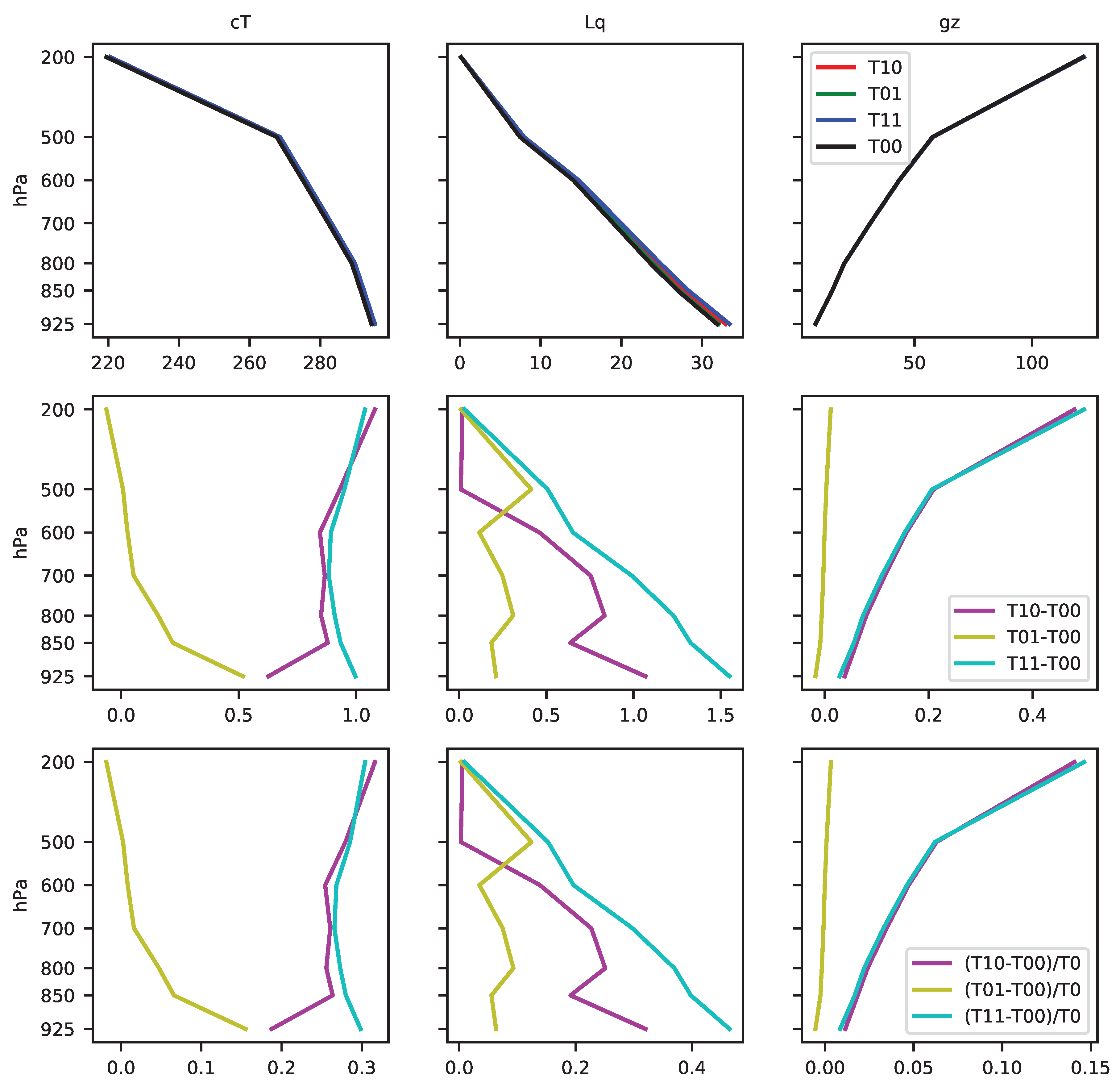
3.2.2. Physical Interpretation
- (i)
- Thermodynamics
- (ii)
- Dynamics
4. Conclusions
4.1. Main Results
- Contrasted responses to the imposed perturbations, with an overall drying tendency of −15% with a warmer atmosphere (T10) and an overall wetting of 17% with a warmer SST (T01), yet with regional discrepancies. Particularly interesting regional features of the rainfall response in these two first experiments are the larger sensitivity of the Guinea region and the sahelian dipole. The combined perturbations experiment (T11) displays a more widespread but smaller wetting tendency of 5%,
- A robust signal, with each experiment resulting in a rainfall anomaly of constant sign in distint synoptic conditions, revealing the strong sensitivity of the rainfall regime to thermodynamical perturbations irrespective of the natural climate variability, most prominently over Guinea,
- A physically consistent model behaviour in response to the boundary forcing perturbations, at least for the mechanisms analyzed and in the range of time and space scales considered,
- Rainfall changes that compare in magnitude with the intrinsic model bias, most prominently over Guinea.
4.2. Limitations and Perspectives
4.2.1. Study Period
4.2.2. Realism of the Perturbations
4.2.3. Results Model-Dependence
4.2.4. Non-Stationary Sensitivity
- precipitation is an “end-of-the-chain” variable: its estimation relies on the faithful representation of many other variables,
- the bulk of rainfall in West Africa is convective, a threshold process.
Author Contributions
Funding
Acknowledgments
Conflicts of Interest
Abbreviations
| AGCM | Atmospheric General Circulation Model |
| AOGCM | Atmosphere-Ocean General Circulation Model |
| CMIP | Coupled Model Intercomparison Project |
| ECMWF | European Centre for Medium-Range Weather Forecasts |
| GCM | General Circulation Model |
| GHG | Green-House Gases |
| ITCZ | Inter-Tropical Convergence Zone |
| MAR | Modèle Atmosphérique Régional |
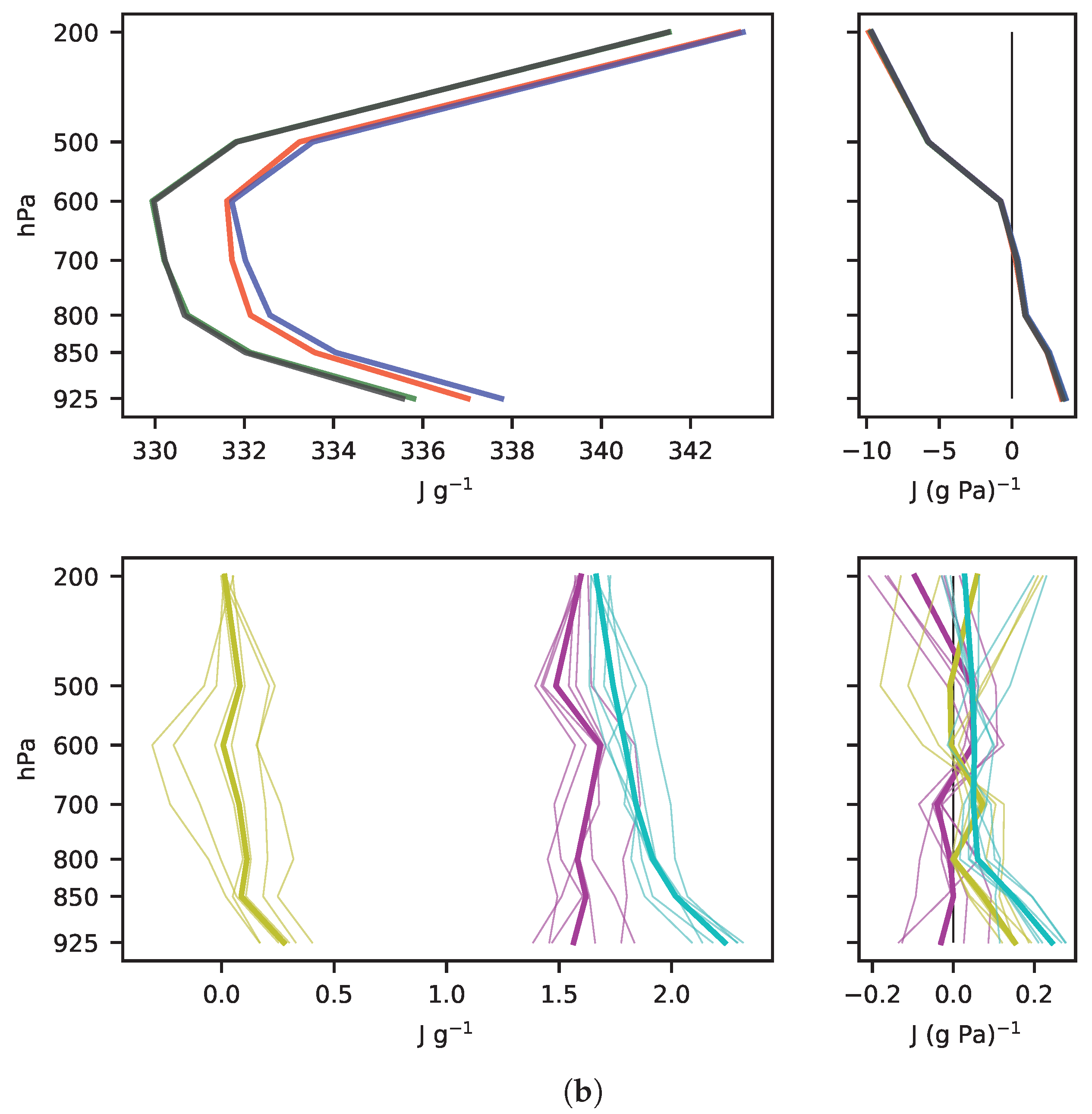
| MSE | Moist Static Energy |
| MSS | Moist Static Stability |
| RCM | Regional Climate Model |
| SCC | Surrogate Climate Change |
| SST | Sea Surface Temperature |
| SVAT | Surface Vegetation Atmosphere Transfer |
| WA | West Africa |
| WAM | West African Monsoon |
Appendix A. JAS Rainfall Anomalies Wrt the Control Simulation (T00): Yearly Values

| Years | Anomalies | Guinea | Sahel | W Sahel | E Sahel |
|---|---|---|---|---|---|
| 1983 | T00 | 340.6 | 303.2 | 280.1 | 327.7 |
| T10-T00 | −79.7 (−23.4) | −21.5 (−7.1) | −45.6 (−16.3) | 4.15 (1.3) | |
| T01-T00 | 104.2 (30.6) | 14.3 (4.7) | 29.9 (10.7) | −2.2 (−0.7) | |
| T11-T00 | 34.2 (10.1) | 6.5 (2.15) | 3.6 (1.3) | 9.6 (−2.9) | |
| 1984 | T00 | 360.4 | 224.3 | 184.4 | 266.6 |
| T10-T00 | −69.8 (−19.4) | −8.1 (−3.5) | −20.9 (−11.3) | 5.5 (2.1) | |
| T01-T00 | 99.9 (27.7) | 2.0 (0.9) | 17.8 (9.7) | −14.8 (−5.5) | |
| T11-T00 | 32.9 (9.12) | 9.3 (4.1) | 9.8 (5.3) | 8.7 (3.3) | |
| 1993 | T00 | 324.0 | 272.8 | 255.3 | 291.3 |
| T10-T00 | −72.5 (−22.4) | −19.1 (−6.9) | −33.4 (−13.3) | −3.3 (−1.1) | |
| T01-T00 | 100.5 (31.0) | 24.6 (9.0) | 40.8 (16.0) | 7.3 (2.5) | |
| T11-T00 | 37.9 (11.7) | 23.8 (8.7) | 28.4 (11.1) | 18.9 −6.5) | |
| 1994 | T00 | 297.4 | 269.3 | 206.8 | 335.5 |
| T10-T00 | −70.6 (−23.8) | −32.0 (−11.9) | −51.6 (−24.9) | −11.2 (−3.2) | |
| T01-T00 | 113.4 (38.1) | 12.0 (4.4) | 25.6 (12.4) | −2.5 (−0.8) | |
| T11-T00 | 38.6 (13.0) | 16.3 (6.1) | 9.61 (4.64) | 23.4 (7.0) | |
| 2010 | T00 | 340.4 | 330.7 | 305.6 | 357.4 |
| T10-T00 | −69.2 (−20.3) | −12.6 (−3.8) | −30.9 (−10.1) | 6.8 (1.9) | |
| T01-T00 | 104.3 (30.7) | 7.25 (2.2) | 17.5 (5.7) | −3.6 (−1.0) | |
| T11-T00 | 39.0 (11.5) | 18.2 (5.5) | 28.0 (9.2) | 7.8 (2.2) | |
| 2011 | T00 | 327.5 | 287.1 | 255.8 | 320.4 |
| T10-T00 | −89.2 (−27.2) | −30.4 (−10.6) | −44.5 (−17.3) | −15.4 (−4.8) | |
| T01-T00 | 92.1 (28.1) | 1.9 (0.7) | 24.2 (9.4) | −21.7 (−6.8) | |
| T11-T00 | 15.6 (4.9) | 15.0 (5.2) | 23.7 (9.3) | 5.76 (1.8) |
Appendix B. JAS Total Rainfall Comparison for the T01 Experiment

Appendix C. 925 hPA Temperature Sensitivity Experiment Anomalies

Appendix D. 925 hPA Relative Humidity Sensitivity Experiment Anomalies

Appendix E. MSE Terms Profiles


References
- Roehrig, R.; Bouniol, D.; Guichard, F.; Hourdin, F.; Redelsperger, J.L. The Present and Future of the West African Monsoon: A Process-Oriented Assessment of CMIP5 Simulations along the AMMA Transect. J. Clim. 2013, 26, 6471–6505. [Google Scholar] [CrossRef]
- Di Baldassarre, G.; Montanari, A.; Lins, H.; Koutsoyiannis, D.; Brandimarte, L.; Blöschl, G. Flood fatalities in Africa: From diagnosis to mitigation. Geophys. Res. Lett. 2010, 37. [Google Scholar] [CrossRef]
- Wilcox, C.; Vischel, T.; Panthou, G.; Bodian, A.; Blanchet, J.; Descroix, L.; Quantin, G.; Cassé, C.; Tanimoun, B.; Kone, S. Trends in hydrological extremes in the Senegal and Niger Rivers. J. Hydrol. 2018, 566, 531–545. [Google Scholar] [CrossRef]
- Trenberth, K.E.; Jones, P.; Ambenje, P.; Bojariu, R.; Easterling, D.; Klein Tank, A.; Parker, D.; Rahimzadeh, F.; Renwick, J.; Rusticucci, M. Observations: Surface and Atmospheric Climate Change. Climate Change 2007: The Physical Science Basis. Contribution of Working Group I to the Fourth Assessment Report of the Intergovernmental Panel on Climate Change; Cambridge University Press: Cambridge, UK; New York, NY, USA, 2007. [Google Scholar]
- Charney, J.G. Dynamics of deserts and drought in the Sahel. Q. J. R. Meteorol. Soc. 1975, 101, 193–202. [Google Scholar] [CrossRef]
- Eltahir, E.A.B.; Gong, C. Dynamics of wet and dry years in West Africa. J. Clim. 1996, 9, 1030–1042. [Google Scholar] [CrossRef]
- Folland, C.K.; Palmer, T.N.; Parker, D.E. Sahel rainfall and worldwide sea temperatures, 1901–85. Nature 1986, 320, 602–607. [Google Scholar] [CrossRef]
- Rowell, D.P. Teleconnections between the tropical Pacific and the Sahel. Q. J. R. Meteorol. Soc. 2001, 127, 1683–1706. [Google Scholar] [CrossRef]
- Giannini, A. Oceanic Forcing of Sahel Rainfall on Interannual to Interdecadal Time Scales. Science 2003, 302, 1027–1030. [Google Scholar] [CrossRef]
- Fontaine, B.; Garcia-Serrano, J.; Roucou, P.; Rodriguez-Fonseca, B.; Losada, T.; Chauvin, F.; Gervois, S.; Sijikumar, S.; Ruti, P.; Janicot, S. Impacts of warm and cold situations in the Mediterranean basins on the West African monsoon: Observed connection patterns (1979–2006) and climate simulations. Clim. Dyn. 2010, 35, 95–114. [Google Scholar] [CrossRef]
- Vizy, E.K.; Cook, K.H. Development and application of a mesoscale climate model for the tropics: Influence of sea surface temperature anomalies on the West African monsoon. J. Geophys. Res. 2002, 107, 4023. [Google Scholar] [CrossRef]
- Messager, C.; Gallée, H.; Brasseur, O. Precipitation sensitivity to regional SST in a regional climate simulation during the West African monsoon for two dry years. Clim. Dyn. 2004, 22, 249–266. [Google Scholar] [CrossRef]
- Giannini, A.; Salack, S.; Lodoun, T.; Ali, A.; Gaye, A.T.; Ndiaye, O. A unifying view of climate change in the Sahel linking intra-seasonal, interannual and longer time scales. Environ. Res. Lett. 2013, 8, 024010. [Google Scholar] [CrossRef]
- Cook, K.H.; Vizy, E.K. Coupled Model Simulations of the West African Monsoon System: Twentieth- and Twenty-First-Century Simulations. J. Clim. 2006, 19, 3681–3703. [Google Scholar] [CrossRef]
- Biasutti, M.; Sobel, A.H.; Camargo, S.J. The Role of the Sahara Low in Summertime Sahel Rainfall Variability and Change in the CMIP3 Models. J. Clim. 2009, 22, 5755–5771. [Google Scholar] [CrossRef][Green Version]
- Lavaysse, C.; Flamant, C.; Janicot, S.; Parker, D.J.; Lafore, J.P.; Sultan, B.; Pelon, J. Seasonal evolution of the West African heat low: A climatological perspective. Clim. Dyn. 2009, 33, 313–330. [Google Scholar] [CrossRef]
- Lavaysse, C.; Flamant, C.; Janicot, S.; Knippertz, P. Links between African easterly waves, midlatitude circulation and intraseasonal pulsations of the West African heat low. Q. J. R. Meteorol. Soc. 2010, 136, 141–158. [Google Scholar] [CrossRef]
- Lebel, T.; Cappelaere, B.; Galle, S.; Hanan, N.; Kergoat, L.; Levis, S.; Vieux, B.; Descroix, L.; Gosset, M.; Mougin, E.; et al. AMMA-CATCH studies in the Sahelian region of West-Africa: An overview. J. Hydrol. 2009, 375, 3–13. [Google Scholar] [CrossRef]
- Evan, A.T.; Flamant, C.; Lavaysse, C.; Kocha, C.; Saci, A. Water Vapor–Forced Greenhouse Warming over the Sahara Desert and the Recent Recovery from the Sahelian Drought. J. Clim. 2015, 28, 108–123. [Google Scholar] [CrossRef]
- Taylor, C.M.; Belušić, D.; Guichard, F.; Parker, D.J.; Vischel, T.; Bock, O.; Harris, P.P.; Janicot, S.; Klein, C.; Panthou, G. Frequency of extreme Sahelian storms tripled since 1982 in satellite observations. Nature 2017, 544, 475–478. [Google Scholar] [CrossRef]
- Gaetani, M.; Flamant, C.; Bastin, S.; Janicot, S.; Lavaysse, C.; Hourdin, F.; Braconnot, P.; Bony, S. West African monsoon dynamics and precipitation: The competition between global SST warming and CO2 increase in CMIP5 idealized simulations. Clim. Dyn. 2017, 48, 1353–1373. [Google Scholar] [CrossRef]
- Giorgi, F. Climate change hot-spots. Geophys. Res. Lett. 2006, 33, L08707. [Google Scholar] [CrossRef]
- Panthou, G.; Vischel, T.; Lebel, T. Recent trends in the regime of extreme rainfall in the Central Sahel. Int. J. Climatol. 2014, 34, 3998–4006. [Google Scholar] [CrossRef]
- Panthou, G.; Lebel, T.; Vischel, T.; Quantin, G.; Sane, Y.; Ba, A.; Ndiaye, O.; Diongue-Niang, A.; Diopkane, M. Rainfall intensification in tropical semi-arid regions: The Sahelian case. Environ. Res. Lett. 2018, 13, 064013. [Google Scholar] [CrossRef]
- Trenberth, K.E.; Dai, A.; Rasmussen, R.M.; Parsons, D.B. The Changing Character of Precipitation. Bull. Am. Meteorol. Soc. 2003, 84, 1205–1218. [Google Scholar] [CrossRef]
- Alpert, P.; Ben-Gai, T.; Baharad, A.; Benjamini, Y.; Yekutieli, D.; Colacino, M.; Diodato, L.; Ramis, C.; Homar, V.; Romero, R.; et al. The paradoxical increase of Mediterranean extreme daily rainfall in spite of decrease in total values. Geophys. Res. Lett. 2002, 29, 1536. [Google Scholar] [CrossRef]
- Alexander, L.V.; Zhang, X.; Peterson, T.C.; Caesar, J.; Gleason, B.; Klein Tank, A.M.G.; Haylock, M.; Collins, D.; Trewin, B.; Rahimzadeh, F.; et al. Global observed changes in daily climate extremes of temperature and precipitation. J. Geophys. Res. 2006, 111, D05109. [Google Scholar] [CrossRef]
- Westra, S.; Alexander, L.V.; Zwiers, F.W. Global Increasing Trends in Annual Maximum Daily Precipitation. J. Clim. 2013, 26, 3904–3918. [Google Scholar] [CrossRef]
- Pall, P.; Allen, M.R.; Stone, D.A. Testing the Clausius–Clapeyron constraint on changes in extreme precipitation under CO2 warming. Clim. Dyn. 2007, 28, 351–363. [Google Scholar] [CrossRef]
- Allen, M.R.; Ingram, W.J. Constraints on future changes in climate and the hydrologic cycle. Nature 2002, 419, 228–232. [Google Scholar] [CrossRef]
- Mekonnen, A.; Thorncroft, C.D.; Aiyyer, A.R. Analysis of Convection and Its Association with African Easterly Waves. J. Clim. 2006, 19, 5405–5421. [Google Scholar] [CrossRef]
- Emori, S.; Brown, S.J. Dynamic and thermodynamic changes in mean and extreme precipitation under changed climate. Geophys. Res. Lett. 2005, 32. [Google Scholar] [CrossRef]
- Rodríguez-Fonseca, B.; Mohino, E.; Mechoso, C.R.; Caminade, C.; Biasutti, M.; Gaetani, M.; Garcia-Serrano, J.; Vizy, E.K.; Cook, K.; Xue, Y.; et al. Variability and Predictability of West African Droughts: A Review on the Role of Sea Surface Temperature Anomalies. J. Clim. 2015, 28, 4034–4060. [Google Scholar] [CrossRef]
- Voldoire, A.; Saint-Martin, D.; Sénési, S.; Decharme, B.; Alias, A.; Chevallier, M.; Colin, J.; Guérémy, J.; Michou, M.; Moine, M.; et al. Evaluation of CMIP6 DECK Experiments With CNRM-CM6-1. J. Adv. Model. Earth Syst. 2019, 11, 2177–2213. [Google Scholar] [CrossRef]
- Wang, Y.; Leung, L.R.; McGregor, J.L.; Lee, D.K.; Wang, W.C.; Ding, Y.; Kimura, F. Regional Climate Modeling: Progress, Challenges, and Prospects. J. Meteorol. Soc. Jpn. Ser. II 2004, 82, 1599–1628. [Google Scholar] [CrossRef]
- Gbobaniyi, E.; Sarr, A.; Sylla, M.B.; Diallo, I.; Lennard, C.; Dosio, A.; Dhiédiou, A.; Kamga, A.; Klutse, N.A.B.; Hewitson, B.; et al. Climatology, annual cycle and interannual variability of precipitation and temperature in CORDEX simulations over West Africa. Int. J. Climatol. 2014, 34, 2241–2257. [Google Scholar] [CrossRef]
- Stratton, R.A.; Senior, C.A.; Vosper, S.B.; Folwell, S.S.; Boutle, I.A.; Earnshaw, P.D.; Kendon, E.; Lock, A.P.; Malcolm, A.; Manners, J.; et al. A Pan-African Convection-Permitting Regional Climate Simulation with the Met Office Unified Model: CP4-Africa. J. Clim. 2018, 31, 3485–3508. [Google Scholar] [CrossRef]
- Giorgi, F.; Mearns, L.O. Introduction to special section: Regional Climate Modeling Revisited. J. Geophys. Res. Atmos. 1999, 104, 6335–6352. [Google Scholar] [CrossRef]
- Pan, Z.; Christensen, J.H.; Arritt, R.W.; Gutowski, W.J.; Takle, E.S.; Otieno, F. Evaluation of uncertainties in regional climate change simulations. J. Geophys. Res. Atmos. 2001, 106, 17735–17751. [Google Scholar] [CrossRef]
- Diallo, F.B.; Hourdin, F.; Rio, C.; Traore, A.K.; Mellul, L.; Guichard, F.; Kergoat, L. The Surface Energy Budget Computed at the Grid-Scale of a Climate Model Challenged by Station Data in West Africa. J. Adv. Model. Earth Syst. 2017, 9, 2710–2738. [Google Scholar] [CrossRef]
- Schär, C.; Frei, C.; Lüthi, D.; Davies, H.C. Surrogate climate-change scenarios for regional climate models. Geophys. Res. Lett. 1996, 23, 669–672. [Google Scholar] [CrossRef]
- Van Lipzig, N.P.M.; Van Meijgaard, E.; Oerlemans, J. Temperature sensitivity of the Antarctic surface mass balance in a regional atmospheric climate model. J. Clim. 2002, 15, 2758–2774. [Google Scholar] [CrossRef]
- Im, E.S.; Coppola, E.; Giorgi, F.; Bi, X. Local effects of climate change over the Alpine region: A study with a high resolution regional climate model with a surrogate climate change scenario. Geophys. Res. Lett. 2010, 37. [Google Scholar] [CrossRef]
- Delhasse, A.; Fettweis, X.; Kittel, C.; Amory, C.; Agosta, C. Brief communication: Impact of the recent atmospheric circulation change in summer on the future surface mass balance of the Greenland Ice Sheet. Cryosphere 2018, 12, 3409–3418. [Google Scholar] [CrossRef]
- Gallée, H.; Schayes, G. Development of a three-dimensional meso-γ primitive equation model: Katabatic winds simulation in the area of Terra Nova Bay, Antarctica. Mon. Weather Rev. 1994, 122, 671–685. [Google Scholar] [CrossRef]
- Kessler, E. On the Distribution and Continuity of Water Substance in Atmospheric Circulations. In Meteorological Monographs; American Meteorological Society: Boston, MA, USA, 1969; Volume 10, pp. 1–84. [Google Scholar]
- Lin, Y.L.; Farley, R.D.; Orville, H.D. Bulk parameterization of the snow field in a cloud model. J. Clim. Appl. Meteorol. 1983, 22, 1065–1092. [Google Scholar] [CrossRef]
- Gallée, H. Simulation of the Mesocyclonic Activity in the Ross Sea, Antarctica. Mon. Weather Rev. 1995, 123, 2051–2069. [Google Scholar] [CrossRef]
- Bechtold, P.; Bazile, E.; Guichard, F.; Mascart, P.; Richard, E. A mass-flux convection scheme for regional and global models. Q. J. R. Meteorol. Soc. 2001, 127, 869–886. [Google Scholar] [CrossRef]
- De Ridder, K.; Schayes, G. The IAGL Land Surface Model. J. Appl. Meteorol. 1997, 36, 167–182. [Google Scholar] [CrossRef]
- Nicholson, S.E. The West African Sahel: A Review of Recent Studies on the Rainfall Regime and Its Interannual Variability. ISRN Meteorol. 2013, 2013, 1–32. [Google Scholar] [CrossRef]
- Duynkerke, P. Application of the E—E turbulence closure model to the neutral and stable atmospheric boundary layer. J. Atmos. Sci. 1988, 45, 865–880. [Google Scholar] [CrossRef]
- Morcrette, J.J. The Surface Downward Longwave Radiation in the ECMWF Forecast System. J. Clim. 2002, 15, 1875–1892. [Google Scholar] [CrossRef]
- Gallée, H.; Moufouma-Okia, W.; Bechtold, P.; Brasseur, O.; Dupays, I.; Marbaix, P.; Messager, C.; Ramel, R.; Lebel, T. A high-resolution simulation of a West African rainy season using a regional climate model. J. Geophys. Res. 2004, 109, D05108. [Google Scholar] [CrossRef]
- Lebel, T.; Diedhou, A.; Laurent, H. Seasonal cycle and interannual variability of the Sahelian rainfall at hydrological scales. J. Geophys. Res. 2003, 108, 8389. [Google Scholar] [CrossRef]
- Ramel, R.; Gallée, H.; Messager, C. On the northward shift of the West African monsoon. Clim. Dyn. 2006, 26, 429–440. [Google Scholar] [CrossRef]
- Dee, D.P.; Uppala, S.M.; Simmons, A.J.; Berrisford, P.; Poli, P.; Kobayashi, S.; Andrae, U.; Balmaseda, M.A.; Balsamo, G.; Bauer, P.; et al. The ERA-Interim reanalysis: Configuration and performance of the data assimilation system. Q. J. R. Meteorol. Soc. 2011, 137, 553–597. [Google Scholar] [CrossRef]
- Gelaro, R.; McCarty, W.; Suárez, M.J.; Todling, R.; Molod, A.; Takacs, L.; Randles, C.A.; Darmenov, A.; Bosilovich, M.G.; Reichle, R.; et al. The Modern-Era Retrospective Analysis for Research and Applications, Version 2 (MERRA-2). J. Clim. 2017, 30, 5419–5454. [Google Scholar] [CrossRef]
- Philippon, N.; Fontaine, B. The relationship between the Sahelian and previous 2nd Guinean rainy seasons: A monsoon regulation by soil wetness? Ann. Geophys. 2002, 20, 575–582. [Google Scholar] [CrossRef]
- Held, I.M.; Soden, B.J. Robust Responses of the Hydrological Cycle to Global Warming. J. Clim. 2006, 19, 5686–5699. [Google Scholar] [CrossRef]
- Funk, C.; Peterson, P.; Landsfeld, M.; Pedreros, D.; Verdin, J.; Shukla, S.; Husak, G.; Rowland, J.; Harrison, L.; Hoell, A.; et al. The climate hazards infrared precipitation with stations—A new environmental record for monitoring extremes. Sci. Data 2015, 2, 150066. [Google Scholar] [CrossRef]
- Ali, A.; Lebel, T.; Amani, A. Rainfall Estimation in the Sahel. Part I: Error Function. J. Appl. Meteorol. 2005, 44, 1691–1706. [Google Scholar] [CrossRef]
- Hersbach, H.; Dee, D. ERA5 reanalysis is in production. ECMWF Newsl. 2016, 147, 5–6. [Google Scholar]
- Flato, G.; Marotzke, J.; Abiodun, B.; Braconnot, P.; Chou, S.C.; Collins, W.; Cox, P.; Driouech, F.; Emori, S.; Eyring, V. Evaluation of climate models. In Climate Change 2013: The Physical Science Basis. Contribution of Working Group I to the Fifth Assessment Report of the Intergovernmental Panel on Climate Change; Cambridge University Press: Cambridge, UK, 2014; pp. 741–866. [Google Scholar]
- Neelin, J.D.; Held, I.M. Modeling tropical convergence based on the moist static energy budget. Mon. Weather Rev. 1987, 115, 3–12. [Google Scholar] [CrossRef]
- Giannini, A. Mechanisms of Climate Change in the Semiarid African Sahel: The Local View. J. Clim. 2010, 23, 743–756. [Google Scholar] [CrossRef]
- Chou, C.; Neelin, J.D. Mechanisms of Global Warming Impacts on Regional Tropical Precipitation. J. Clim. 2004, 17, 14. [Google Scholar] [CrossRef]
- Hill, S.A.; Ming, Y.; Held, I.M.; Zhao, M. A Moist Static Energy Budget–Based Analysis of the Sahel Rainfall Response to Uniform Oceanic Warming. J. Clim. 2017, 30, 5637–5660. [Google Scholar] [CrossRef]
- Seth, A.; Rauscher, S.A.; Rojas, M.; Giannini, A.; Camargo, S.J. Enhanced spring convective barrier for monsoons in a warmer world?: A letter. Clim. Chang. 2011, 104, 403–414. [Google Scholar] [CrossRef]
- Romps, D.M. Response of Tropical Precipitation to Global Warming. J. Atmos. Sci. 2011, 68, 123–138. [Google Scholar] [CrossRef]
- Kawase, H.; Yoshikane, T.; Hara, M.; Kimura, F.; Yasunari, T.; Ailikun, B.; Ueda, H.; Inoue, T. Intermodel variability of future changes in the Baiu rainband estimated by the pseudo global warming downscaling method. J. Geophys. Res. 2009, 114, D24110. [Google Scholar] [CrossRef]
- Doutreloup, S.; Wyard, C.; Amory, C.; Kittel, C.; Erpicum, M.; Fettweis, X. Sensitivity to Convective Schemes on Precipitation Simulated by the Regional Climate Model MAR over Belgium (1987–2017). Atmosphere 2019, 10, 34. [Google Scholar] [CrossRef]
- Nikulin, G.; Jones, C.; Giorgi, F.; Asrar, G.; Büchner, M.; Cerezo-Mota, R.; Christensen, O.B.; Déqué, M.; Fernandez, J.; Hänsler, A.; et al. Precipitation Climatology in an Ensemble of CORDEX-Africa Regional Climate Simulations. J. Clim. 2012, 25, 6057–6078. [Google Scholar] [CrossRef]
- Maraun, D. Nonstationarities of regional climate model biases in European seasonal mean temperature and precipitation sums. Geophys. Res. Lett. 2012, 39. [Google Scholar] [CrossRef]
- Krinner, G.; Flanner, M.G. Striking stationarity of large-scale climate model bias patterns under strong climate change. Proc. Natl. Acad. Sci. USA 2018, 115, 9462–9466. [Google Scholar] [CrossRef] [PubMed]


| Datasets | WA | Guinea | Sahel | |
|---|---|---|---|---|
| MAR (T00) | mean | 362 | 428 | 299 |
| CHIRPS | mean | 483 | 672 | 415 |
| difference | −113 | −244 | −116 | |
| % change | −25 | −36 | −28 | |
| spatial c | 0.67 | 0.63 | 0.75 | |
| BADOPLU | mean | 453 | 575 | 438 |
| difference | −91 | −147 | −139 | |
| % change | −20 | −26 | −32 | |
| spatial c | 0.67 | 0.59 | 0.71 | |
| ERA5 | mean | 446 | 650 | 315 |
| difference | −84 | −222 | −16 | |
| % change | −19 | −34 | −5 | |
| spatial c | 0.64 | 0.52 | 0.72 |
| Anomalies | Guinea | Sahel | W Sahel | E Sahel |
|---|---|---|---|---|
| T00 | 428 | 299 | 282 | 314 |
| T10-T00 | −75.2 (−22.7) | −20.6 (−7.3) | −37.9 (−15.3) | −2.2 (−0.7) |
| T01-T00 | 102.4 (30.9) | 10.3 (3.7) | 26.0 (10.5) | −6.3 (−2.0) |
| T11-T00 | 33.1 (10.0) | 14.8 (5.3) | 17.2 (6.9) | 12.4 (3.9) |
© 2020 by the authors. Licensee MDPI, Basel, Switzerland. This article is an open access article distributed under the terms and conditions of the Creative Commons Attribution (CC BY) license (http://creativecommons.org/licenses/by/4.0/).
Share and Cite
Chagnaud, G.; Gallée, H.; Lebel, T.; Panthou, G.; Vischel, T. A Boundary Forcing Sensitivity Analysis of the West African Monsoon Simulated by the Modèle Atmosphérique Régional. Atmosphere 2020, 11, 191. https://doi.org/10.3390/atmos11020191
Chagnaud G, Gallée H, Lebel T, Panthou G, Vischel T. A Boundary Forcing Sensitivity Analysis of the West African Monsoon Simulated by the Modèle Atmosphérique Régional. Atmosphere. 2020; 11(2):191. https://doi.org/10.3390/atmos11020191
Chicago/Turabian StyleChagnaud, Guillaume, Hubert Gallée, Thierry Lebel, Gérémy Panthou, and Théo Vischel. 2020. "A Boundary Forcing Sensitivity Analysis of the West African Monsoon Simulated by the Modèle Atmosphérique Régional" Atmosphere 11, no. 2: 191. https://doi.org/10.3390/atmos11020191
APA StyleChagnaud, G., Gallée, H., Lebel, T., Panthou, G., & Vischel, T. (2020). A Boundary Forcing Sensitivity Analysis of the West African Monsoon Simulated by the Modèle Atmosphérique Régional. Atmosphere, 11(2), 191. https://doi.org/10.3390/atmos11020191