Pollution Transport Patterns Obtained Through Generalized Lagrangian Coherent Structures

Abstract

Identifying atmospheric transport pathways is important to understand the effects of pollutants on weather, climate, and human health. The atmospheric wind field is variable in space and time and contains complex patterns due to turbulent mixing. In such a highly unsteady flow field, it can be challenging to predict material transport over a finite-time interval. Particle trajectories are often used to study how pollutants evolve in the atmosphere. Nevertheless, individual trajectories are sensitive to their initial conditions. Lagrangian Coherent Structures (LCSs) have been shown to form the template of fluid parcel motion in a fluid flow. LCSs can be characterized by special material surfaces that organize the parcel motion into ordered patterns. These key material surfaces form the core of fluid deformation patterns, such as saddle points, tangles, filaments, barriers, and pathways. Traditionally, the study of LCSs has looked at coherent structures derived from integrating the wind velocity field. It has been assumed that particles in the atmosphere will generally evolve with the wind. Recent work has begun to look at the motion of chemical species, such as water vapor, within atmospheric flows. By calculating the flux associated with each species, a new effective flux-based velocity field can be obtained for each species. This work analyzes generalized species-weighted coherent structures associated with various chemical species to find their patterns and pathways in the atmosphere, providing a new tool and language for the assessment of pollutant transport and patterns.

1. Introduction

Eulerian chemical transport models such as the Community Multiscale Air Quality (CMAQ) modeling system [1] are powerful tools to simulate the transport and fate of air pollutants at various scales from local to global. Informed by meteorological drivers such as the Weather Research and Forecasting (WRF) model [2], these models calculate the advection of gases and aerosols in the atmosphere and provide information about how pollutants are transported from one location to another.

Identifying atmospheric transport pathways and barriers is important to understand pollutants’ effects on weather, climate, and human health. The atmospheric wind field is variable in space and time and contains complex patterns due to turbulent mixing. In such a highly unsteady flow field, streamlines (Eulerian entities showing the local direction of the velocity at any given instant) do not provide useful information regarding the transport over a finite time. Therefore, air parcel trajectories are often used to study how pollutants move in the atmosphere [3]. Nevertheless, individual trajectories are sensitive to their initial conditions [4,5], cannot fully resolve the complexity of the flow, and often result in a chaotic and tangled field that is difficult to analyze [6]. Therefore, a more systematic and robust approach is needed. Rather than individual trajectories, the qualitative properties of entire air masses, approximated as a continuum of closely spaced trajectories, are more reliable.

Lagrangian Coherent Structures (LCSs) have been shown to form the template of fluid tracer motion in a continuum flow. LCSs can be characterized by special material surfaces that organize the tracer motion into ordered patterns [7,8,9,10,11]. These key material surfaces form the core of fluid deformation patterns, such as saddle points, tangles, filaments, and jets. In environmental and geophysical settings, the LCS approach has had success in understanding certain transport events, like the polar vortex (ozone hole) split [11,12], oil spill spread [7,13,14], the spread of radioactive waste from a reactor disaster [15], airborne spread of invasive microorganisms [9,16], and atmospheric rivers [17].

When working with approximate models (e.g., WRF or CMAQ data), there is the issue of whether the data used to compute LCS are representative of the actual flow. Small errors in the velocity field typically result in large integrated errors for trajectories [18], but only result in small errors in the LCS because LCSs depict divergent and convergent flow behavior, mathematically classified as “hyperbolic” regions in the flow, which have been proven to be robust to errors [19]. Thus, even if trajectories obtained from numerically integrating flow fields from approximate models show noticeable deviations from actual tracer paths, one can expect the computed LCSs to be close to true ones present in the flow. Such studies have been performed and validated, for example, for approximate geophysical flows from data [10,20,21,22].

Traditionally, the study of atmospheric LCSs has looked at coherent structures derived from integrating the wind velocity field [9,11,16,23,24,25]. The underlying assumption is that the scalar of interest evolves along air parcel trajectories. However, chemical species in the atmosphere may evolve according to more complicated laws, such as coupled reaction-advection-diffusion equations, and do not necessarily follow air parcels. We can therefore consider generalized LCS, following Balasuriya et al. [26], which is a framework for quantities, such as chemical species, particulates, and pollutants, which are not fully locked to the underlying fluid. For instance, recent work has begun to look at the motion of chemical species, such as water vapor, within atmospheric flows [17].

This present paper looks at analyzing coherent structures associated with generalized velocity fields derived from the flux of various chemical species, to find geographic regions over which each species will be attracted (or dispersed) over short times (≤6 h). The paper is organized as follows. In Section 2, we introduce the numerical air quality model used, define the column-averaged flux-based effective velocity field for each species, define the instantaneous attraction (and repulsion) rate based on the gradient tensor of the effective velocity field, and relate it to the finite-time Lyapunov exponent field and its ridges, which are the hyperbolic attracting (and repelling) LCS of interest. In Section 3, we discuss the results of applying the analysis of concentrations of various chemical species (H${}_2$O, SO${}_2$, O${}_3$, SO${}_4^{2-}$, NO${}_2$, and Na${}^{+}$) during a typical weekday over a region of the southeastern United States. In Section 4, we provide conclusions and prospects for future work.

2. Methods

2.1. Air Quality Model

Simulations were conducted using the CMAQ v5.2 [27,28] regional chemical transport model for a domain covering the southeastern United States extending approximately from ${88}^{°}$ W to ${75}^{°}$ W in longitude and from ${29}^{°}$ N to ${88}^{°}$ N in latitude. CMAQ is driven by the meteorological data from WRF v3.7 [2]. The temporal resolution was 1 h, the horizontal resolution 12 km, and the vertical resolution 35 pressure layers, with higher resolution near the surface extending up to 50 hPa (height between layers varying from 0.05 to 1 km). The key WRF physics options, including the Pleim–Xiu Land Surface Model (PX LSM) with indirect soil nudging, the Asymmetric Convective Model Version 2 (ACM2) for the planetary boundary layer, the Rapid Radiative Transfer Model (RRTM) for radiation, Version 2 of the Kain–Fritsch (KF2) cumulus parameterization, and the Morrison double-moment cloud microphysics scheme (see [28] for associated references), were chosen based on a previously evaluated configuration of WRF for air quality studies [29,30].

The CMAQ model was configured with the updated Carbon-Bond 6 (CB6r3) for gas-phase chemistry. Emissions were based on the 2011 National Emissions Inventory Version 2, as well as the windblown dust emission scheme of Foroutan et al. [31] and the bidirectional (emissions and deposition) ammonia exchange of Pleim et al. [32]. Boundary conditions for these simulations were provided by a hemispheric CMAQ run. The model configuration was described in and evaluated by several previous studies [27,33,34].

In this study, we chose 1 July 2011 as our test case. This was an arbitrary choice since the focus of the present work was to show the general applicability of the generalized LCS framework. Investigations of weather patterns in the domain for this day indicated (1) a generally calm surface wind throughout the day, (2) an onshore surface wind on the east coast of the United States in the afternoon, (3) a jet stream with wind speed as high as 80 kt at 200 hPa, and (4) a trough at 200 hPa associated with the jet stream covering much of the southeast United States and the Atlantic Ocean. It should be noted, however, that species transport occurs on various layers of the atmosphere and, therefore, weather patterns on a single layer are not sufficient to draw a full picture of pollution transport. Instead, we developed species-weighted column-averaged generalized velocity fields as described below.

2.2. Species-Weighted Column-Averaged Generalized Velocity Field

Consider a horizontal wind velocity vector $\mathbf{v}(\mathbf{x},\eta ,t)=\left(u\right(\mathbf{x},\eta ,t),v(\mathbf{x},\eta ,t\left)\right)$, where u is the eastward wind component and v is the northward wind component, which varies spatiotemporally in all three dimensions. Here, t is time in an interval $I=[t_{\min },t_{\max }]$, $\mathbf{x}=(x,y)\in U$ (where U is a portion of the surface of a sphere ${\mathbb{S}}^2$ at generalized height $\eta$) is the horizontal position vector, where x is the eastward position and y is the northward position, measured in longitude and latitude, respectively, and $\eta$ is a non-dimensional vertical coordinate, which varies from zero at the surface to one at 50 hPa (about 19 km above sea level).

Following [17], a generalized velocity field is derived from the system,

$$\begin{array}{cc}\hfill Q^s(\mathbf{x},t)& =\frac{1}{g}{\int }_0^1{q}^s(\mathbf{x},\eta ,t)\frac{\partial p}{\partial \eta }(\mathbf{x},\eta ,t)d\eta \hfill \end{array}$$

(1)

$$\begin{array}{cc}\hfill {\mathsf{\Phi }}_x^s(\mathbf{x},t)& =\frac{1}{g}{\int }_0^{1}u(\mathbf{x},\eta ,t)q^s(\mathbf{x},\eta ,t)\frac{\partial p}{\partial \eta }(\mathbf{x},\eta ,t)d\eta \hfill \end{array}$$

(2)

$$\begin{array}{cc}\hfill {\mathsf{\Phi }}_y^s(\mathbf{x},t)& =\frac{1}{g}{\int }_0^{1}v(\mathbf{x},\eta ,t)q^s(\mathbf{x},\eta ,t)\frac{\partial p}{\partial \eta }(\mathbf{x},\eta ,t)d\eta \hfill \end{array}$$

(3)

where $Q^s$ is the column-integrated species amount for chemical species s (measured as a surface density in kg/m${}^2$), ${\mathit{\Phi }}^s(\mathbf{x},t)=({\mathsf{\Phi }}_x^s(\mathbf{x},t),{\mathsf{\Phi }}_y^s(\mathbf{x},t))$ is the eastward and northward species fluxes, respectively, which depend on $\mathbf{x}$ and t, and g is the constant gravitational acceleration. Here, $p(\mathbf{x},\eta ,t)$ is the pressure and $q^s(\mathbf{x},\eta ,t)$ is the mixing ratio, i.e., the ratio of the mass of species s to the total mass of the air parcel located at $(\mathbf{x},\eta )$ at time t.

For our analysis, we considered the following column-averaged flux-based effective velocity field for species s,

$${\mathbf{v}}^s(\mathbf{x},t)=\frac{1}{Q^s(\mathbf{x},t)}{\mathit{\Phi }}^s(\mathbf{x},t).$$

(4)

Following [17], when the wind velocity fields were vertically averaged in this way, the pressure layers were weighted according to their chemical species content, such that ${\mathbf{v}}^s$ was representative of the dynamics of the transport of the chemical species in question. The resultant effective species advection equation for species s is,

$$\begin{array}{c}\hfill \frac{d}{dt}\mathbf{x}={\mathbf{v}}^s(\mathbf{x},t),\\ \hfill {\mathbf{x}}_0=\mathbf{x}\left(t_0\right).\end{array}$$

(5)

In this system, $\mathbf{x}\left(t\right)$ is the position vector of an air parcel containing the species s at time t and ${\mathbf{v}}^s(\mathbf{x},t)$ is the effective flux-based velocity of species s or just effective velocity at position $\mathbf{x}$ and time t.

2.3. Eulerian-Lagrangian Analysis

Due to their chaotic nature, time dependent unsteady fluid flows such as atmospheric flows can be challenging to analyze. As mentioned in the Introduction, the method of LCS has become a popular tool to analyze the transport of particles in such flows. A common computational framework to obtain LCS is to consider a scalar field derived from numerically integrated Lagrangian trajectories (i.e., the numerical approximation of the solutions of (5)), in particular the Finite-Time Lyapunov Exponent (FTLE) field [10,11].

New Eulerian tools have recently been developed, which use velocity gradients, instead of integrating particle trajectories, which approximate an instantaneous limit of FTLE and LCS. These velocity gradients are assembled into the Eulerian rate-of-strain tensor, ${\mathbf{S}}^s$, discussed below. In [35], it was shown that the Eulerian rate-of-strain tensor can provide an instantaneous approximation of the Lagrangian dynamics of a fluid flow and states that one should seek objective Eulerian coherent structures (OECSs) based on it, as short-term limits of LCSs. Further work on this topic [36] also showed that in two-dimensional flows, the minimum and maximum eigenvalues of the Eulerian rate-of-strain tensor are the limits of the backward-time and forward-time FTLE fields, respectively, as integration (advection) time goes to zero. Nolan et al. [36] posited that the trenches of the minimum eigenvalue field can be identified as instantaneous attracting LCSs and the ridges of the maximum eigenvalue field can be identified as instantaneous repelling LCSs. For the remainder of the paper, we shall refer to the minimum and maximum eigenvalues of the Eulerian rate-of-strain tensor as the attraction and repulsion rates, respectively, and both can be considered as instantaneous, rather than finite-time, Lyapunov exponents.

For our analysis, we considered the fluid particle advection dynamical system, Equation (5). We analyzed this system by looking at the attraction rate, which was the minimum eigenvalue, $s_1^s$, of the Eulerian rate-of-strain tensor for species s,

$${\mathbf{S}}^s(\mathbf{x},t)=\frac{1}{2}\left(\nabla {\mathbf{v}}^s(\mathbf{x},t)+\nabla {\mathbf{v}}^s{(\mathbf{x},t)}^T\right).$$

(6)

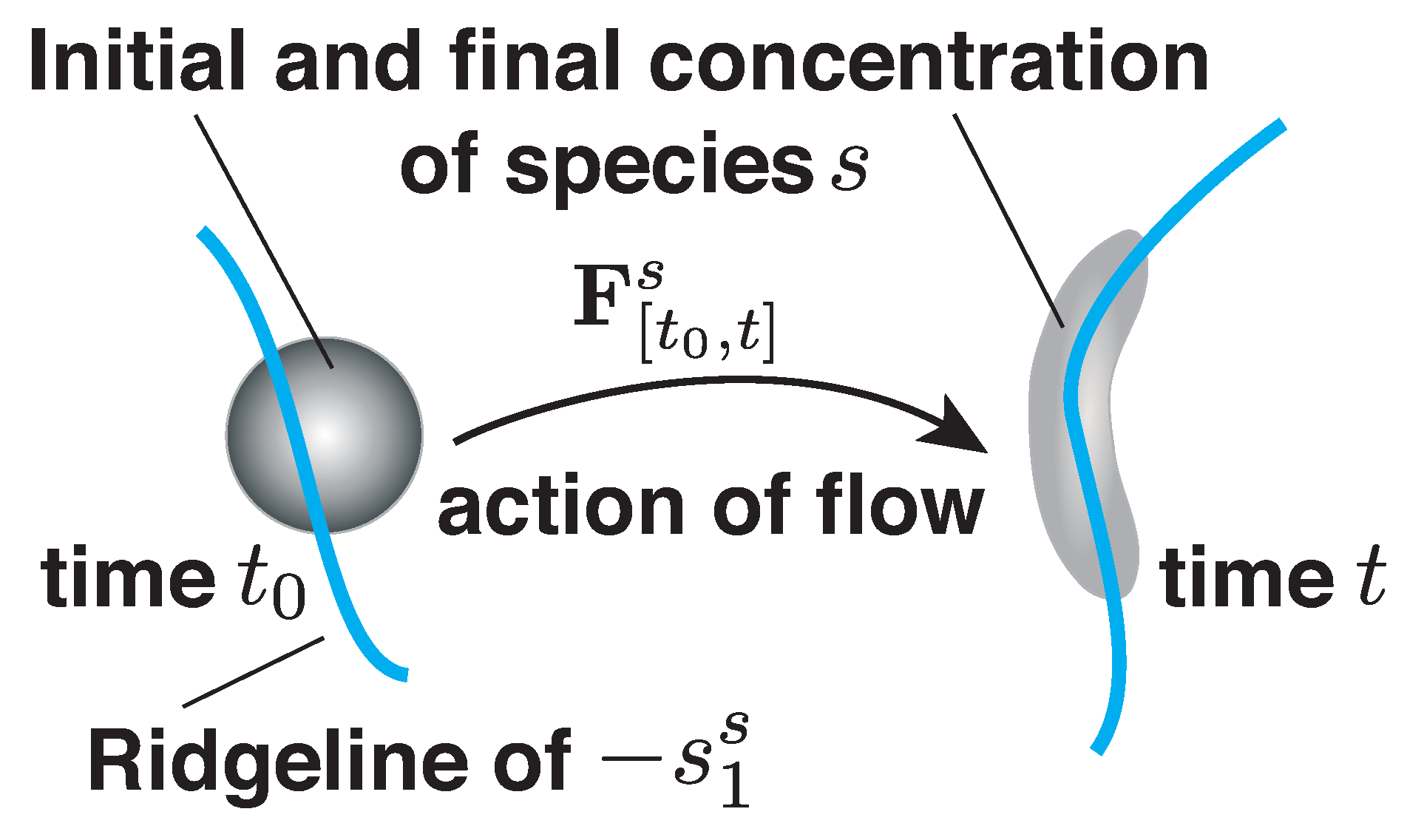
As stated before, the attraction rate provides a means of identifying the attracting OECSs, which are the instantaneous LCSs. The attraction rate provides information on where material particles and species concentrations will converge, as shown in the schematic of Figure 1. The lower the value of the (negative) attraction rate, the more particles will be attracted to that point. We focused on the attraction rate given its importance for predicting enhanced concentrations of atmospherically advected tracers, as nearby particles will converge onto those features and flow with them as opposed to repelling features, which particles will diverge from before flowing independent of those features.

2.4. Computation of Effective Velocity Gradient and Instantaneous Attraction Rate

In order to calculate the attraction rate, we first needed to calculate the gradient of the wind velocity field, $\nabla \mathbf{v}(\mathbf{x},t)$, for the spatiotemporally varying wind velocity vector $\mathbf{v}(\mathbf{x},t)=(u,v)$, where u is the eastward wind component and v is the northward wind component.

This method could then be applied to ${\mathbf{v}}^s(\mathbf{x},t)=(u^s(\mathbf{x},t),v^s(\mathbf{x},t))$ as well to get the full horizontal gradient of the effective species flux velocity vector,

$$\nabla {\mathbf{v}}^s(\mathbf{x},t)=\left[\begin{array}{cc}\frac{\partial u^s}{\partial x}& \frac{\partial u^s}{\partial y}\\ \frac{\partial v^s}{\partial x}& \frac{\partial v^s}{\partial y}\end{array}\right],$$

(7)

and the Eulerian rate-of-strain tensor,

$${\mathbf{S}}^s(\mathbf{x},t)=\left[\begin{array}{cc}\frac{\partial u^s}{\partial x}& \frac{1}{2}\left(\frac{\partial u^s}{\partial y}+\frac{\partial v^s}{\partial x}\right)\\ \frac{1}{2}\left(\frac{\partial u^s}{\partial y}+\frac{\partial v^s}{\partial x}\right)& \frac{\partial v^s}{\partial y}\end{array}\right].$$

(8)

The attraction rate, $s_1^s(\mathbf{x},t)$, which is the minimum eigenvalue of ${\mathbf{S}}^s(\mathbf{x},t)$ at the location and time $(\mathbf{x},t)$, is given analytically by,

$$s_1^s(\mathbf{x},t)=\frac{1}{2}\left(\frac{\partial u^s}{\partial x}+\frac{\partial v^s}{\partial y}\right)-\frac{1}{2}\sqrt{{\left(\frac{\partial u^s}{\partial x}-\frac{\partial v^s}{\partial y}\right)}^2+{\left(\frac{\partial u^s}{\partial y}+\frac{\partial v^s}{\partial x}\right)}^2},$$

(9)

where the dependence of $u^s$ and $v^s$ on $\mathbf{x}$ and t is understood. This can be written more succinctly in terms of fluid quantities,

$$s_1^s(\mathbf{x},t)=\frac{1}{2}\left(\nabla ·{\mathbf{v}}^s-{\epsilon }_T^s\right),$$

(10)

where,

$$\nabla ·{\mathbf{v}}^s(\mathbf{x},t_0)=\frac{\partial u^s}{\partial x}+\frac{\partial v^s}{\partial y},$$

(11)

is the divergence of the effective flow field, ${\epsilon }_N^s(\mathbf{x},t_0)=\frac{\partial u^s}{\partial x}-\frac{\partial v^s}{\partial y}$ is the normal component of effective strain, ${\epsilon }_S^s(\mathbf{x},t_0)=\frac{\partial u^s}{\partial y}+\frac{\partial v^s}{\partial x}$ is the shear component of effective strain, and,

$${\epsilon }_T^s(\mathbf{x},t_0)=\sqrt{{\left({\epsilon }_N^s(\mathbf{x},t_0)\right)}^2+{\left({\epsilon }_S^s(\mathbf{x},t_0)\right)}^2},$$

(12)

is the total effective strain. Note that, in general, the column-averaged effective species flux velocity ${\mathbf{v}}^s$ is not a divergence-free vector field. Furthermore, one can define the repulsion rate, $s_2^s(\mathbf{x},t)$, as the maximum eigenvalue of ${\mathbf{S}}^s(\mathbf{x},t)$.

2.5. Computation of the Lagrangian Trajectory-Averaged Attraction Rate

Based on the effective species advection Equation (5), we can analyze the system over time using Lagrangian (particle trajectory) methods, by first calculating the flow map, ${\mathbf{x}}_0\mapsto {\mathbf{x}}_t={\mathbf{F}}_{[t_0,t]}^s\left({\mathbf{x}}_0\right)$, for some time interval of interest, $[t_0,t]\subset I$. If the final time t is less than the initial time, $t_0$, then back-trajectories are calculated, which give information about the regions of trajectory-averaged attraction. The flow map for species s, ${\mathbf{F}}_{[t_0,t]}^s:U\to U$, is given by,

$${\mathbf{F}}_{[t_0,t]}^s\left({\mathbf{x}}_0\right)={\mathbf{x}}_0+{\int }_{t_0}^t{\mathbf{v}}^s({\mathbf{F}}_{[t_0,\tau ]}^s\left({\mathbf{x}}_0\right),\tau )d\tau ,$$

(13)

and is typically given numerically [10,37,38,39]. Taking the gradient of the flow map ${\mathbf{F}}_{[t_0,t]}^s\left({\mathbf{x}}_0\right)$ with respect to initial conditions ${\mathbf{x}}_0$, $\nabla {\mathbf{F}}_{[t_0,t]}^s\left({\mathbf{x}}_0\right)$, the right Cauchy–Green strain tensor over a time interval of interest can be calculated,

$${\mathbf{C}}_{[t_0,t]}^s\left({\mathbf{x}}_0\right)=\nabla {\mathbf{F}}_{[t_0,t]}^s{\left({\mathbf{x}}_0\right)}^T·\nabla {\mathbf{F}}_{[t_0,t]}^s\left({\mathbf{x}}_0\right),$$

(14)

which is positive-definite, giving eigenvalues that are all positive. In a two-dimensional flow, the two eigenvalues are ordered ${\lambda }_1^s<{\lambda }_2^s$. From the maximum eigenvalue, ${\lambda }_2^s$, the FTLE [10,40] can be defined as,

$${\sigma }_{[t_0,t_0+T]}^s\left({\mathbf{x}}_0\right)=\frac{1}{2|T|}log\left({\lambda }_2^s\right),$$

(15)

where $T=t-t_0$ is the (signed) elapsed time, often referred to as the integration time or evolution time in the FTLE literature. The FTLE measures the rate of separation of two nearby fluid parcels in a flow over the time horizon T. Ridges of the ${\sigma }_{[t_0,t_0+T]}^s\left({\mathbf{x}}_0\right)$ field for $T<0$ identify regions of the flow that are the most attracting over the time interval $[t_0,t_0+T]$. Furthermore, in [36], it was demonstrated that the $-s_1^s({\mathbf{x}}_0,t_0)$ field (with the minus sign) was the limit of the ${\sigma }_{[t_0,t_0+T]}^s\left({\mathbf{x}}_0\right)$ field as $T\to 0$. Thus, the attraction rate field, $-s_1^s({\mathbf{x}}_0,t_0)$, provides a computationally inexpensive instantaneous approximation of the main attracting curves, as it is based on a single velocity snapshot, and no particle trajectory integration is necessary. Indeed, the FTLE can be viewed as a Lagrangian trajectory-averaged attraction rate (i.e., a path-integrated attraction rate; cf. [41]), but many of the short-time features are already visible in the instantaneous attraction rate field.

In this study, the initial time for all calculations was $t_0=$ 21:00 UTC 01 July 2011 (17:00 Eastern Daylight Time). For each species, we used integration times T of 0 h, −1 h, and −6 h. For $T=0$ h, we used the attraction rate, which did not require trajectory integration and gave an instantaneous approximation of transport structures occurring over time scales on the order of hours.

2.6. Correlation of Column-Averaged Transport Structures with Wind-Only Structures at a Fixed Pressure Layer

Some chemical species have their transport correlated with different heights over different time scales. For instance, a pollutant produced near the surface may stay near the surface over a short time, but reach great altitudes with time. Some chemical species may be correlated with sources from the stratosphere. To quantify this, we will look at the correlation of the wind-only FTLE at a fixed pressure layer with the column-averaged FTLE and attraction rate fields for various species, and over multiple time scales. We calculated the correlation coefficient between FTLE field from the species-weighted vertically-integrated velocity field and the FTLE fields for each individual vertical level for integration times T of 0 h, −1 h, and −6 h. A high correlation at a pressure level suggested that the chemical species transport was most influenced by the wind at that pressure level.

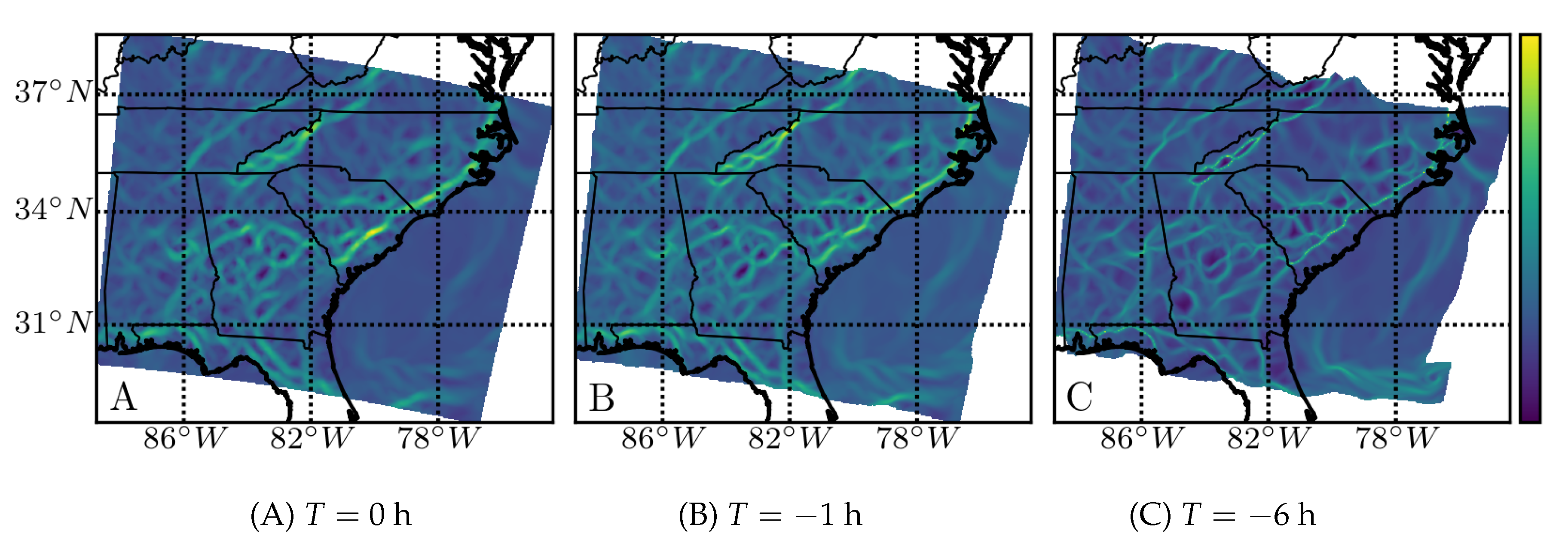
As an example of a wind-only structure, we show in Figure 2 the attracting FTLE fields calculated based on the horizontal wind vector components for a pressure layer corresponding to approximately 100 m AGL. High FTLE values (attracting regions) are shown in yellow.

The (Pearson) correlation of the finite-time Lyapunov exponent field (Panels (B) and (C)) with the instantaneous Lyapunov exponent, the attraction rate, $-s_1$ (Panel (A)), was visibly high. The correlation coefficient (not depicted) showed a monotonically decreasing correlation as $|T|$ increased, but stayed above 50% for $|T|<$ 6 h.

3. Results and Discussion

We considered the transport of the following chemical species: water vapor (H${}_2$O), sulfur dioxide (SO${}_2$), ozone (O${}_3$), sulfate (SO${}_4^{2-}$), nitrogen dioxide (NO${}_2$), and sodium (Na${}^{+}$).

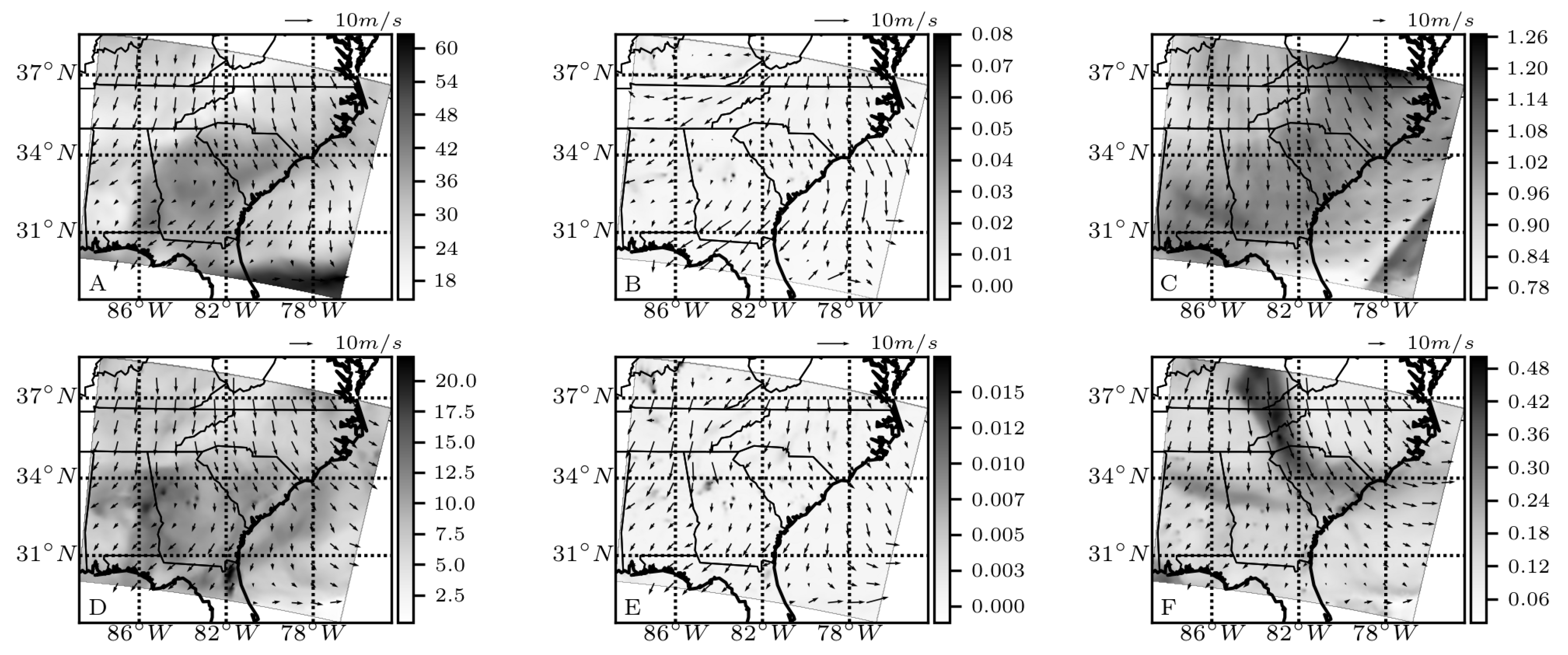
Figure 3 shows the column-integrated species amount $Q^s$ for the six chemical species considered in this study superimposed with their vector fluxes ${\mathit{\Phi }}^s$, at the initial time, $t_0$. High concentrations of water vapor were seen over the ocean, as well as along the Atlantic coastal plain. As expected, the areas of high concentrations for pollutants such as SO${}_2$, SO${}_4^{2-}$, and NO${}_2$ were associated with urban regions in the southeast United States [42,43]. High ozone and sodium regions, on the other hand, were due to plumes transporting these species aloft.

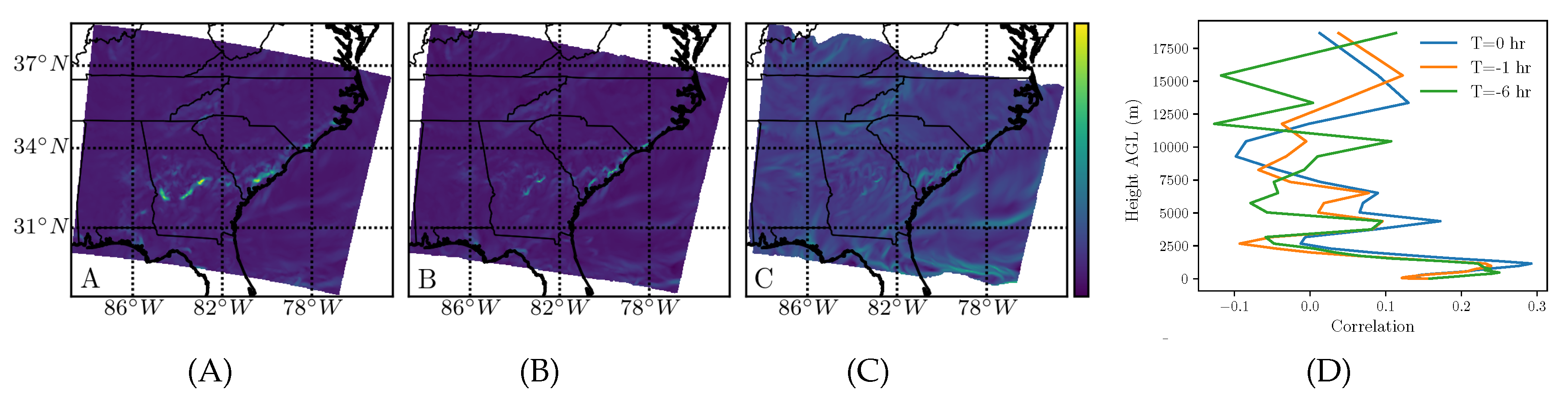
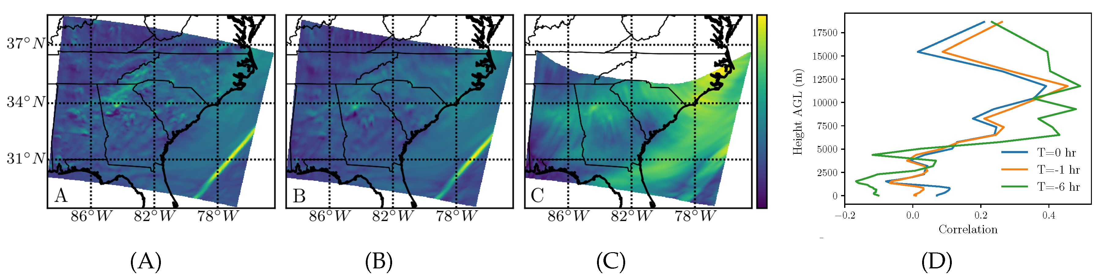
We calculated the FTLE based on the column-averaged generalized velocity fields, Equation (4). For column-averaged water vapor transport, the comparison of the backward-time FTLE field for the three integration times is shown in Figure 4A–C.

The correlation with the wind-only FTLE is shown in (D), revealing high correlation in the troposphere for all three time scales and then a slight peak around 8.25 km at the longest time scale (6 h). Further analysis suggested that the peak may be associated with a southerly jet stream aloft transporting water vapor. Furthermore, notice the nearly linear inland attracting filament parallel to the South Carolina and North Carolina coasts, which was in both the water vapor attraction fields for 0 and $-1$ h (Figure 4A,B) and also the corresponding low altitude wind-only attraction fields (Figure 2A,B). The filament seemed to follow the front due to the onshore winds blowing from the Atlantic Ocean.

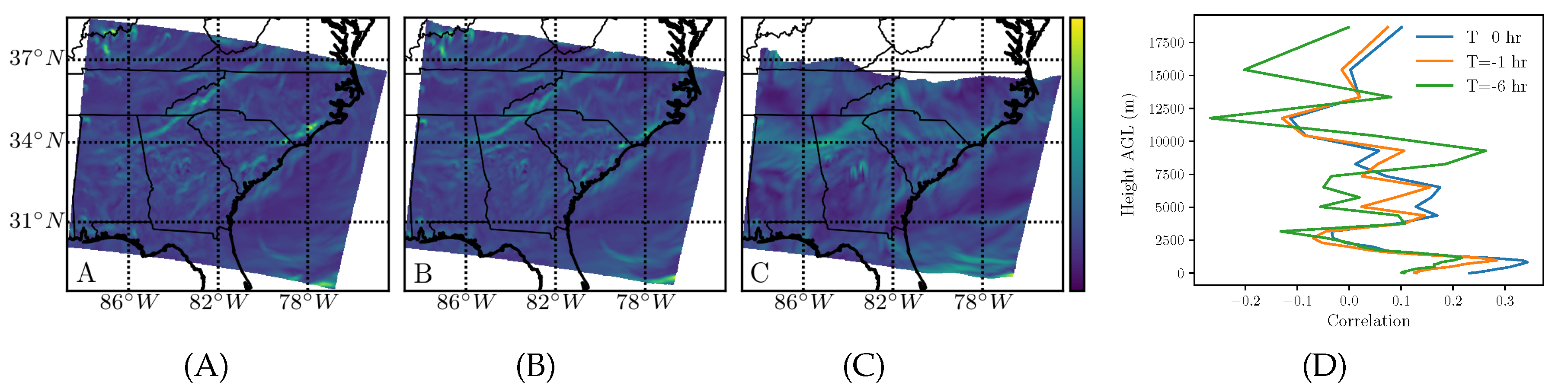
Sulfur dioxide is an industrial pollutant, toxic to humans, and causes acid rain. The comparison of the backward-time FTLE field for the three integration times is shown in Figure 5A–C. The correlation with the wind-only FTLE is shown in (D), revealing that the highest correlation for sulfur dioxide was in the troposphere for all three times. Note, however, that the highest correlation was only about 0.3, half the maximum for water vapor in Figure 4D.

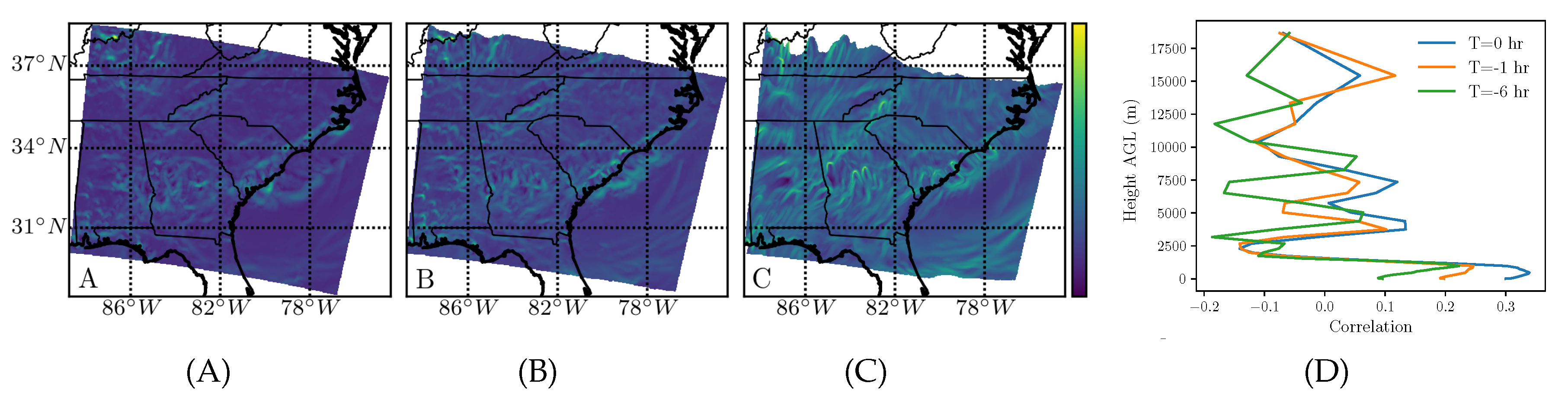
Ozone is naturally occurring at high altitudes and absorbs ultraviolet radiation. It is also a pollutant at low altitudes, created by chemical reactions between volatile organic compounds and oxides of nitrogen. It causes respiratory irritation and reduces lung function. The comparison of the backward-time FTLE field for the three integration times is shown in Figure 6A–C. The correlation with the wind-only FTLE is shown in (D), revealing a high correlation in the upper troposphere for all three times, with a small peak in the lower troposphere only for the instantaneous attraction rate. The strong attraction region over the ocean in (A)–(C) corresponds to the trough observed at 200 hPa, the extent of which is clearly highlighted in (C). This feature manifests itself as a peak at around 12 km (≈200 hPa) in (D) for all three times.

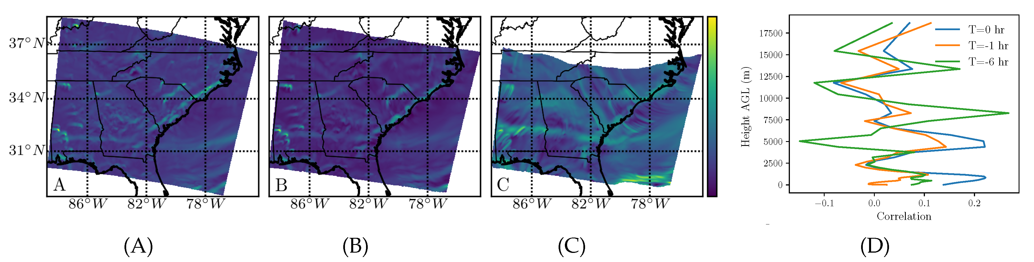
Sulfate is a particulate pollutant that causes respiratory irritation and acid rain. The comparison of the backward-time FTLE field for the three integration times is shown in Figure 7A–C.

The correlation with the wind-only FTLE is shown in (D), revealing a high correlation in the troposphere over short times (0–1 h) and then a peak around 10 km at the longer time scale (6 h).

Nitrogen dioxide is a highly reactive gas that may cause respiratory symptoms such as acute bronchitis. Figure 8A–C shows the backward-time FTLE field for the three integration times, and the correlation with the wind-only FTLE is shown in (D). The attracting regions seemed to be more scattered for nitrogen dioxide, which may be attributed to its scatted sources along roads and highways, as a major source of NO${}_2$ is the exhaust of motor vehicles. The correlation coefficients revealed that NO${}_2$ transport was mostly influenced by the near surface winds.

Particulate sodium in the atmosphere is mainly derived from natural sources including sea salt and mineral dust. The backward-time FTLE fields in Figure 9A–C show a strong attracting filament parallel to the coasts of North and South Carolina, similar to what was observed for water vapor (Figure 4). This might be related to the sea salt emissions and transport by onshore winds. Another attracting region extending across Alabama and Georgia is observed in Figure 9C. Further investigations revealed that this attracting filament lied on a pressure level aloft and was associated with long-range transport of sodium into the domain in higher altitudes. This was further confirmed by a high correlation coefficient at around 8.25 km for the longest time scale (6 h) as shown in (D).

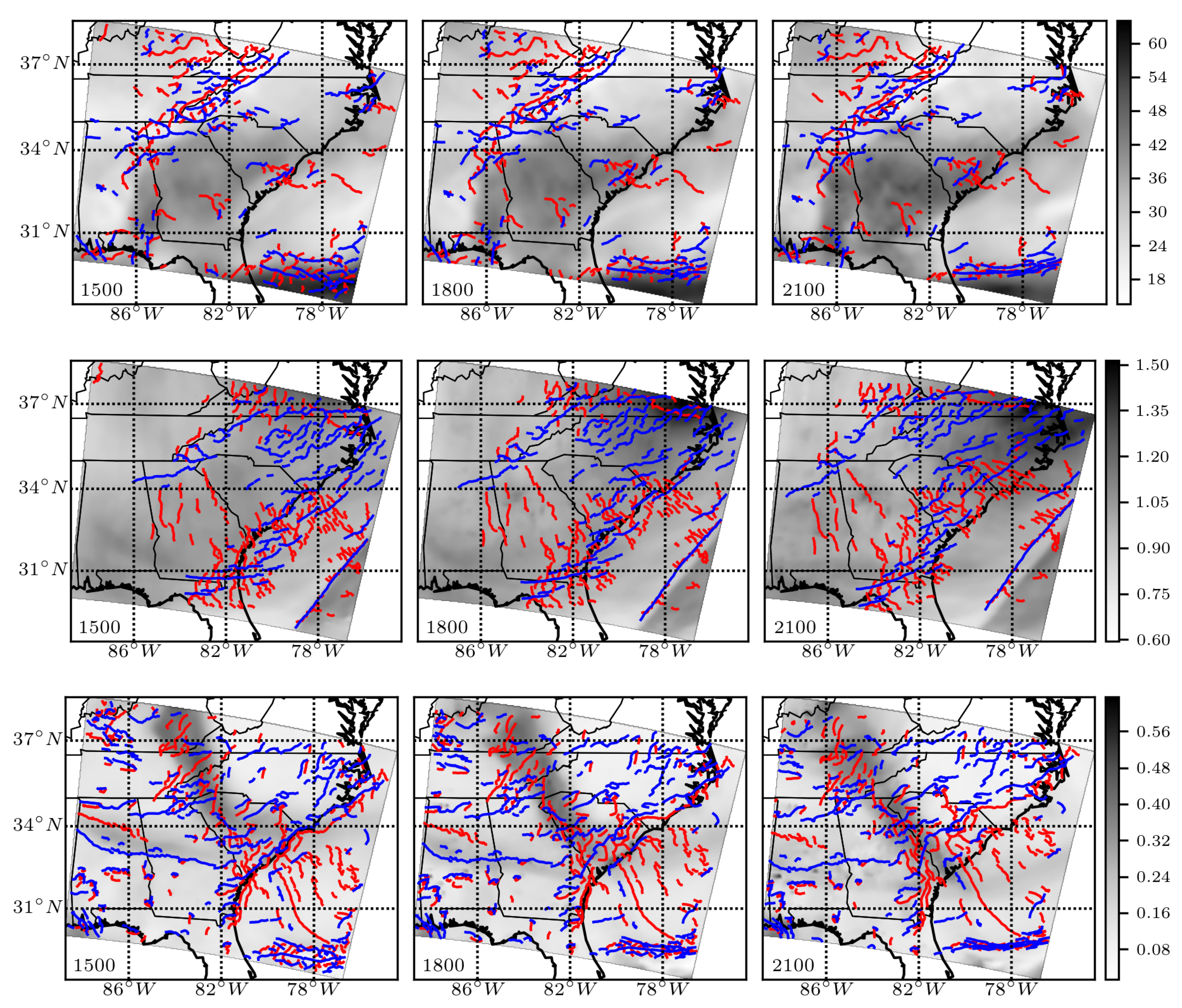
To illustrate the predictive ability of the ridges of the $-s_1$ and $s_2$ fields to capture the dominant behavior in the vertically-integrated species amounts, we overlaid them, in blue and red, respectively, over the species amount at the initial time, 15:00, for water vapor, in the top left of Figure 10.

Superimposed on the $Q^s$ field are the attracting (blue) and repelling (red) instantaneous hyperbolic LCSs, material lines within the flow where the attraction and repulsion of each species will be maximized. These features were obtained using a ridge detection algorithm [36] (an averaging or coarse-graining procedure could be performed, revealing fewer structures [11,44,45]). In the top center, we show the species amount for water vapor 3 h later, at 18:00, with the 15:00 $-s_1$ and $s_2$ ridgelines advected to 18:00. In the top right, we show the species amount for water vapor three additional hours later, at 21:00, with the 15:00 $-s_1$ and $s_2$ ridgelines advected to 21:00. The middle panel shows the same, but for ozone (O${}_3$), and the bottom panel for sodium (Na${}^{+}$).

Notice that features in the species concentration field tended to correspond to the attracting and repelling LCSs. Furthermore, notice that despite being advected by the same time varying wind field, with its own passive tracer FTLE field (see Figure 2), these three species had quite different patterns of high attraction and repulsion. Water vapor had a group of features along the Appalachian mountain range inland, as well as a large attracting east-west feature off the coast. Ozone had a main group of features along the coast, as well as an attracting southwest-northeast feature off the coast. Sodium also had a main group of features along the coast, but also two main inland features nearly perpendicular to the coast. Like water vapor, sodium also had a large attracting east-west feature off the coast. While one can seek to understand the pollutant attraction and repulsion features in terms of weather phenomena at various scales (e.g., baroclinic waves, jets, mesoscale winds), previous work showed that atmospheric LCSs were not necessarily related to obvious weather phenomena (e.g., storms or cold fronts) [9,46]. They could also be short-lived, appearing perhaps for just hours before disappearing [16] and, in other cases, persisting for hours, or recurring in a regular pattern [47].

4. Conclusions

In this paper, we demonstrated the ability of short-time and instantaneous generalized LCSs [26] to predict atmospheric transport for several air pollutants and particulates. We took inspiration from an earlier study focused on the global-scale transport of water vapor [17] and generalized the approach to other chemical species. We used a column-averaged atmospheric effective velocity field for each species, along with species-specific flow maps, to compute effective FTLE fields. The ridgelines of the backward (forward) FTLE field formed species-specific attracting (repelling) atmospheric structures. Due to a variety of factors, different species had different effective velocity fields and therefore different transport structures of attraction of repulsion. We also compared species-weighted vertically-integrated atmospheric transport structures to wind-only transport structures as a function of height, to reveal altitudes that were important for the transport of each species.

This study revealed promise for using LCS as a tool for short-term prediction of patterns of concentrations of pollutants and particulates. This approach overcame some limitations of looking at individual trajectories, which could be prone to error. LCS, being based on the motion of a continuum (rather than individual trajectories) and based on the locally hyperbolic behavior of that continuum (in the sense of dynamics), are more robust to error [19,48].

Future work will extend the analysis to various vertical layers and a fully three-dimensional analysis. We will also extend this analysis to other test cases over various temporal and spatial scales, develop LCS based on field measurements, combine this with data from simulations [49,50], compare LCS forecasts with satellite and remote sensing observations (e.g., as done for ozone in [11]), and study the implication of LCS (weighted by various species) to source locations, atmospheric chemistry, and exposure [5,9].