Study on the Sensitivity of Summer Ozone Density to the Enhanced Aerosol Loading over the Tibetan Plateau

Abstract

The existence of the Asian tropopause aerosol layer (ATAL) and the influence of the heterogeneous chemistry of aerosols on the summer ozone valley over the Tibetan Plateau have received continuous attention. In this paper, based on the established box model of the heterogeneous chemical reactions of stratospheric ozone and comparative simulation and sensitivity tests, the influence of heterogeneous chemical reactions of possible aerosols over the Tibetan Plateau on the ozone valley is analyzed and evaluated. The preliminary results show that from May to August, the change in the temperature and pressure field has little effect on the ozone valley, and the lower the temperature is, the higher the ozone concentration. The temperature itself has a negative correlation with ozone chemistry. The influence ratio of heterogeneous chemical reactions on the ozone valley from May to August is approximately 0.5–17%, and the maximum in June is approximately 5%. With the decrease in monsoon convection, the influence ratio of heterogeneous chemical reactions increases.

1. Introduction

Since scientists discovered the ozone hole in Antarctica [1], and the ozone depletion phenomenon in winter in the Arctic [2], the phenomenon of low ozone values has also been found over the “Third Pole” of the world over the Tibetan Plateau. Zhou et al. [3] analyzed the temporal and spatial changes in the total ozone in China using the data of TOMS (Total Ozone Mapping Spectrometer). It was found that an obvious low center value of the total ozone began to appear over the Tibetan Plateau in June every year, which was called the “ozone valley”.

Based on analysis of the mechanism of the ozone valley, it is considered that the unique topography and the special dynamic and thermal effects in summer are the main factors in its formation [4,5,6,7,8]. Liu et al. [9] simulated the ozone valley by using a three-dimensional chemical transport model (OSLO CTM2). The main idea is that the dynamic transport process plays the most important role in the formation of the ozone valley; furthermore, the chemical process can also not be ignored.

Satellite observations and model simulations show that the convective activity associated with the South Asian summer monsoon is an important channel for transporting air from the lower troposphere to the stratosphere [10,11,12,13,14]. When tropospheric air is effectively transported to the stratosphere, it also transports anthropogenic emissions near the surface layer to the upper troposphere and lower stratosphere (UTLS) region, which will affect the atmospheric chemical processes there [15].

Moreover, the Asian tropopause aerosol layer (ATAL) has been observed in summer since the late 1990s [16,17]. Through analysis of Lidar data, it is found that the aerosol scattering coefficient of the ATAL undergoes obvious seasonal changes: it is high in summer and autumn and low in winter and spring, and the peak value is mainly in July and August after all the volcanic ash effects are eliminated. The ATAL is different from the Junge’s aerosol layer [18]. The latter is mainly affected by volcanic eruption (especially tropical volcanic activity) [19,20,21], and the ATAL may be primarily caused by the deep convective activity over the Indian subcontinent, which transports the surface layer pollutants to the UTLS area [22].

Heterogeneous chemical reactions on the aerosols of polar stratospheric clouds, such as

ClONO₂(g) + H₂O(s)→HOCl(g) + HNO₃(g)

(1)

N₂O₅(g) + H₂O(s)→2 HNO₃(g)

(2)

play an important role in ozone depletion in Antarctica [23,24]. The ATAL is greatly influenced by human activities and may have many kinds of aerosols. The heterogeneous chemical reactions on aerosols may influence the formation of the summer ozone valley over the Tibetan Plateau, but the influence ratio has not been quantitatively evaluated. Therefore, in this paper, we use the established box model of the heterogeneous chemical reactions of ozone in the lower stratosphere and satellite observation data to conduct a preliminary study on the above issues.

2. Introduction of Data and the Model

2.1. Satellite Data

In this paper, the V6.2 data of the stratospheric aerosol and gas test instrument (SAGE II) on the ERBS (Earth Radiation Budget Satellite) are used. By observing seven bands (385, 448, 453, 525, 600, 940 and 1020 nm) of the sun’s edge detection, the vertical profiles of ozone, aerosol, nitrogen dioxide, water vapor and temperature are retrieved. The data period was from January 1988 to August 2005. The satellite operates in an orbit with an inclination of 57° and a height of 610 km [25,26]. The authors of [27] compared the data measured by SAGE II and POAM (Polar Ozone and Aerosol Measurement) III and concluded that in the middle latitude region, the SAGE data were more reliable than the POAM data.

The ozone change and difference curve of the two regions observed by satellite is shown in Figure 1. It can be seen that most of the ozone difference between the two regions occurs in May to August, i.e., the ozone valley in summer, while in December, January and February, the ozone concentration over the Tibetan Plateau is slightly higher than the Pacific Ocean region at the same latitude. As shown in Figure 1, the ozone concentration is low in summer and autumn, but high in winter and spring, regardless of whether the data are from inside or outside the plateau. This is because the height of 18 km is in the lower stratosphere and because the concentration of ozone increases with increasing height. The tropopause rises in summer and autumn and declines in winter and spring [28].

According to the analysis of the SAGE II data, due to the influence of monsoon convection, the pressure amplitude in the lower stratosphere over the Tibetan Plateau is larger than that in the lower stratosphere over the region at the same latitude outside the Tibetan Plateau (as shown in Figure 2a). Compared with other regions at the same latitude, the Tibetan Plateau displays an obvious low temperature phenomenon in summer (as shown in Figure 2b). The temperature and air pressure will affect the content of H₂SO₄ in sulfuric acid droplets [23], thus affecting the heterogeneous chemical reaction rate. The temperature itself also affects the thermochemical reaction rate, leading to different ozone chemical equilibria. The aerosol area index in the lower stratosphere over the Tibetan Plateau has an obvious single-peak distribution in summer and autumn (as shown in Figure 2c); the lowest value is approximately 0.73 × 10⁻⁸ cm²/cm³, and the peak value is approximately 2 × 10⁻⁸ cm²/cm³. The aerosol area index over the Pacific Ocean region at the same altitude (as shown in Figure 2c black solid line) has little seasonal variation: it is slightly higher in summer and lower in other seasons, with an average value of 0.73 × 10⁻⁸ cm²/cm³.

2.2. Model Description

The box model of the heterogeneous chemical reactions of stratospheric ozone used in this paper was established by Yang and Brasseur in 1994 [29]. It can simulate the average situation of the heterogeneous chemistry of stratospheric ozone ignoring the effects of atmospheric dynamics [30,31]. In this paper, the model was further improved by adding related species of carbon groups and heterogeneous chemical reaction modules of different aerosols.

The current box model includes six groups of chemical species: oxygen group (O₃, O_1D, O, O₂), hydrogen group (H₂O, HO, HO₂, H₂O₂), nitrogen group (NO, NO₂, NO₃, N₂O₅, HNO₂, HNO₃, HO₂NO₂), chlorine group (Cl, ClO, ClO₂, Cl₂, Cl₂O₂, HCl, HOCl, ClONO₂), bromine group (Br, BrO, Br₂, HBr, HOBr, BrONO₂, BrCl) and carbon group (CH₄, CO, CO₂, CH₃O₂, CH₂O, CH₃COOH). There are 36 substances in total, and three kinds of chemical reactions involved, which have 26 photochemical reactions (Table S1 in the supplement), 99 thermochemical reactions (Table S2 in the supplement) and 11 heterogeneous chemical reactions (

Table 1. Related parameters of heterogeneous chemical reactions on different aerosols.

Chemical Reaction	Sulfuric Acid Droplets (gam)	Solid Sulfuric Acid Salt (Stkcf)	OC (Stkcf)	BC (Stkcf)	Sea Salt (Stkcf)	Mineral Dust (Stkcf)
NO2 + 0.5 × H2O→0.5 HNO3 + 0.5 HNO2	1× 10−4	1 × 10−4	1 × 10−4	1 × 10−4	1 × 10−4	1 × 10−4
NO3 + H2O→HNO3 + OH	1× 10−1	1 × 10−1	1 × 10−1	1 × 10−1	1 × 10−1	1 × 10−1
N2O5 + H2O→2 HNO3	f(p, t)	4 × 10−3	2.6 × 10−4	5 × 10−3	5 × 10−3	1 × 10−2
HOCl + HCl→Cl2 + H2O	f(p, t)	8 × 10−1
HOCl + HBr→BrCl + H2O		8 × 10−1
ClONO2 + H2O→HOCl + HNO3	f(p, t)	1 × 10−4
ClONO2 + HCl→Cl2 + HNO3	f(p, t)	1 × 10−5
HOBr + HCl→BrCl + H2O	f(p, t)	8 × 10−1
HOBr + HBr→Br2 + H2O		2 × 10−1			2 × 10−1
BrONO2 + H2O→HOBr + HNO3	f(p, t)	8 × 10−1			3 × 10−1
BrONO2 + HCl→BrCl + HNO3	9 × 10−1	9 × 10−1

Note: (1) The formula of function f(p, t) in the table is omitted, in which p represents the air pressure and t represents the air temperature, and the parameters of gam and S_tkcf are dimensionless; (2) All the heterogeneous chemical reactions, parameters and the function f(p, t) listed in the table refer to GEOS-Chem code and were derived from Kirner’s paper [38] and JPL [39].

).

The input parameters of the model include the source intensity and loss rate of nitrogen oxides, chlorides and bromides. The environmental parameters of the model include the solar radiation spectrum, air pressure, air temperature, aerosol area index, H₂O and O₂.

2.3. Aerosol and Heterogeneous Chemical Reactions

For the aerosol composition and proportion of the ATAL, some scholars have made observations and simulations, but their results are different. Vernier et al. [22] found that the main components of the aerosols in the lower layer of the ATAL are carbonaceous compounds and sulfides. Yu et al. [32] used a sectional aerosol model (Community Aerosol and Radiation Model for Atmospheres (CARMA)) coupled with the Community Earth System Model version 1 (CESM1) to study the chemical composition and optical properties of the NATAL (tropopause aerosol layer in North America) and ATAL. It is shown that the main components of the ATAL are sulfate, organic matter discharged from the surface and secondary organic matter. Gu et al. [33] used the global three-dimensional Goddard Earth Observing System chemical transport model (GEOS-Chem) to examine the contribution of nitrate aerosols to aerosol concentrations in the upper troposphere and lower stratosphere (UTLS) over the Tibetan Plateau and the South Asian summer monsoon (TP/SASM) region during the summer of 2005. The simulation results show that the aerosol concentrations of sulfate, nitrate, ammonium, black carbon, organic carbon and PM_2.5 in the UTLS over the Tibetan Plateau and the South Asian monsoon region in summer are elevated and that nitrate is the most dominant aerosol species.

Therefore, influenced by the monsoon convection, on the one hand, the lower stratosphere over the Tibetan Plateau appears to have an obvious low temperature in summer, and the minimum of the average value is approximately 200 K (Figure 2b). This temperature range may make the binary solution (H₂SO₄/H₂O) absorb the gas-phase HNO₃ and gradually generate the ternary solution: HNO₃/H₂SO₄/H₂O [34,35,36]. Combined with the multiyear temperature observed by SAGE II (figure omitted), the minimum daily average temperature can sometimes reach 196 K. Therefore, it is considered that there may be stratospheric liquid aerosol (SLA) (including binary sulfuric acid solution (H₂SO₄/H₂O) and ternary supercooling solution: HNO₃/H₂SO₄/H₂O) and solid sulfuric acid salt (SAT: H₂SO₄·4H₂O). On the other hand, due to the strong upward movement, the aerosol emitted from the earth's surface is transported from the troposphere to the lower stratosphere [37], so the influence of organic carbon, black carbon, sea salt and mineral dust aerosols should also be considered.

The rate of heterogeneous chemical reactions on liquid aerosols is obtained with Equation (3):

$$\mathrm{Rate}\_\mathrm{liquid}\left(\mathrm{l}\right)=\mathrm{gam}\times 1\times {10}^{-8}\times \mathrm{velo}\times \mathrm{A}/4$$

(3)

where rate is in cm³/molecular/s; A is the total surface area of the aerosol in unit volume, in cm²/cm³; A/4 is the total collision area; gam is a dimensionless probability that a gaseous molecule collides with an aerosol particle and leads to a chemical reaction and generally considered as a function of temperature and air pressure (Table 1). Temperature and air pressure will affect the content of sulfuric acid in the sulfuric acid droplets, thus affecting the heterogeneous chemical reaction rate. The velo is the average rate of molecular thermal motion, calculated by Equation (4):

$$\mathrm{velo}={\left(8kT/\pi M\right)}^{1/2}$$

(4)

where k is the Boltzmann constant; T is the air temperature; and M is the molecular mass of the gas (unit: g/mol).

The rate of heterogeneous chemical reactions on the surface of solid aerosols is obtained with:

$$\mathrm{Rate}\_\mathrm{solid}\left(\mathrm{s}\right)=\mathrm{A}\times 1\times {10}^{-8}/(\mathrm{R}/D_{fkg}+2.749064\times {10}^{-4}\times {\mathrm{M}}^{1/2}/\left(S_{tkcf}\times {\mathrm{T}}^{1/2}\right)$$

(5)

$$D_{fkg}=9.45\times {10}^{17}/{\mathrm{D}}_{enair}\times {\mathrm{T}}^{1/2}\times {\left(3.472\times {10}^{-2}+1/\mathrm{M}\right)}^{1/2}$$

(6)

Here, A is the same as in Equation (3); R is the aerosol radius, in $\mathsf{\mu }\mathrm{m}$; T is the same as in Equation (4); D_fkg is the gas diffusion coefficient, in cm²/s; D_enair is the air molecular number density, in cm⁻³; and S_tkcf is the sticking coefficient, which is dimensionless and can be obtained from the experimental data (Table 1).

3. Simulation and Result

Considering that the largest difference in ozone number concentration at the altitude of 18 km between the same latitude region and Tibetan Plateau occurs in summer [40] and that the aerosol of the ATAL is mainly concentrated in 13–19 km [41,42,43], the ozone heterogeneous chemical reaction box model will be established at the height of 18 km in the two regions. Through comparative simulation and sensitivity tests, we will analyze and evaluate the influences of the temperature and pressure field in the lower stratosphere over the Tibetan Plateau and of the heterogeneous chemical reactions of aerosols on the ozone valley.

First, the geodetic coordinates of the Tibetan Plateau are 25–40° N, 70–110° E, and the coordinates of the comparative region at the same latitude are 25–40° N, 140–180° E, which is located in the Middle East of the Pacific Ocean and is not affected by the topography, the South Asia High, monsoon convection and the ATAL.

The temperature and pressure field of the comparative region at the same latitude observed by satellite is brought into the model, and the parameters are adjusted so that it can simulate the change in ozone and other chemical substances there. Second, the temperature and pressure field of the Tibetan Plateau is brought into the model, and the influence of the temperature and pressure field itself on the ozone valley is obtained.

Then, the potential aerosols of the ATAL are added to the box model in turn. The influence of heterogeneous chemical reactions on the summer ozone valley of the Tibetan Plateau are separately analyzed and evaluated through sensitivity tests.

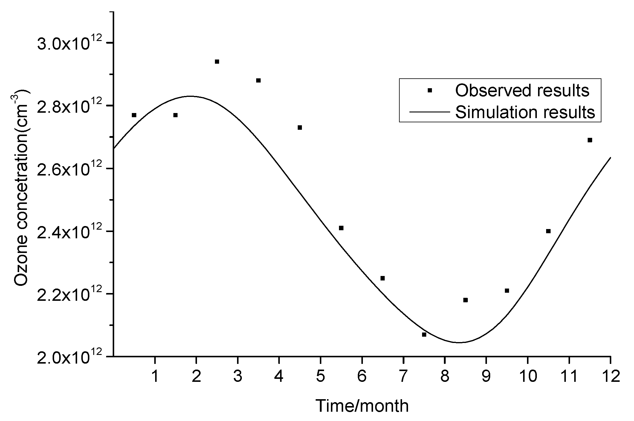
3.1. Simulation Test

Because the two regions (Tibetan Plateau (25–40° N, 70–110° E) and the comparative region over the Pacific Ocean (25–40° N, 140–180° E)) are at the same latitude (25–40° N) and height (18 km), we use the solar spectrum of 32° N at the altitude of 18 km as the model’s spectral input value. The specific value is calculated by the medium spectral resolution atmospheric transmittance and radiation transfer algorithm software Modtran4.0 developed by the Air Force Research Laboratory of the United States.

Considering that the ATAL was discovered after 1998, we used the air temperature, air pressure, water vapor mixture ratio and aerosol area index of the SAGE-II satellite of the two regions at the height of 18 km in 1998–2005. These observations are averaged on a monthly basis in their respective geographical regions, and their time curves in one year are obtained. The changes in air pressure, temperature and aerosol area index are shown in Figure 2. Because of the influence of monsoon convection on the Tibetan Plateau, the temperature pressure field and aerosol area index are considerably different from those of the region at the same latitude, so different values are used in the simulation. Because the photochemical lifetime of O₂ is up to 10 years, the same constant value of 4.00 × 10¹⁷ cm⁻³ is used in the model. The number concentration of H₂O is converted from the water vapor mixture ratio at 18 km altitude observed by SAGE II. According to the time curve of the H₂O value at 18 km altitude obtained from the analysis of satellite data, there is no obvious seasonal difference between the two regions, and the curves are almost the same. Therefore, the same value is adopted. At the altitude of 18 km in the comparative region at the same latitude, which is not affected by the topography and monsoon convection, the background aerosol is sulfuric acid droplets.

Due to the lack of actual observed values of aerosols at present, to separately obtain the influence of heterogeneous chemical reactions of aerosols on the ozone valley, the source strength and loss rate of the box model in the two regions are taken as constant (as shown in

Table 2. Input parameters of the box model.

Parameter	Value	Parameter	Value
SNOx	15 cm−3 s−1	DHNO3	0.55 × 10−8 s−1
SClOx	55 cm−3 s−1	DHCl	0.40 × 10−7 s−1
SBrOx	13 cm−3 s−1	DHBr	0.50 × 10−7 s−1
SCH4	2000 cm−3 s−1	DCO2	0.40 × 10−7 s−1

) when simulating the actual situation and do not change with time. When the input parameters of the model are taken as the values in Table 2, the simulated ozone and other atmospheric fractional concentrations are compared with the results of other models, as shown in

Table 3. Comparison of the simulation results from different models.

	O3	HOX	NOX	ClOX	BrOX	HNO3	ClONO2	BrONO2	CH4
(1)	2.55 × 1012	7.43 × 106	2.66 × 109	1.57 × 106	—	9.08 × 109	9.3 × 107	—	4.29 × 1012
(2)	3.48 × 1012	1.87 × 106	2.76 × 109	1.25 × 106	—	2.21 × 1010	9.01 × 107	—	3.02 × 1012
(3)	2.96 × 1012	6.15 × 106	5.83 × 108	1.48 × 107	4.27 × 107	4.49 × 109	2.12 × 108	5.93 × 106	4.30 × 1012
(4)	2.32 × 1012	3.24 × 106	8.09 × 108	2.46 × 107	2.90 × 107	3.91 × 109	1.48 × 108	1.33 × 107	2.43 × 1012

(1) The results of Orlando J [44]; (2) the results given by Wang [30]; (3) the results given by NCAR's Socrates; (4) the result of the model simulation in this paper. The results in the table are the number concentration of each component in the same latitude region at the 18 km height and summer solstice, unit: cm⁻³.

.

The scattered points in Figure 3 are the observed results over the Pacific Ocean region, and the curve is the simulation results obtained using the box model established in this paper. It can be seen from Table 3 and Figure 3 that, in general, the box model is able to simulate the time variation in ozone and other substances over the Pacific Ocean region and the average state of various substances in summer.

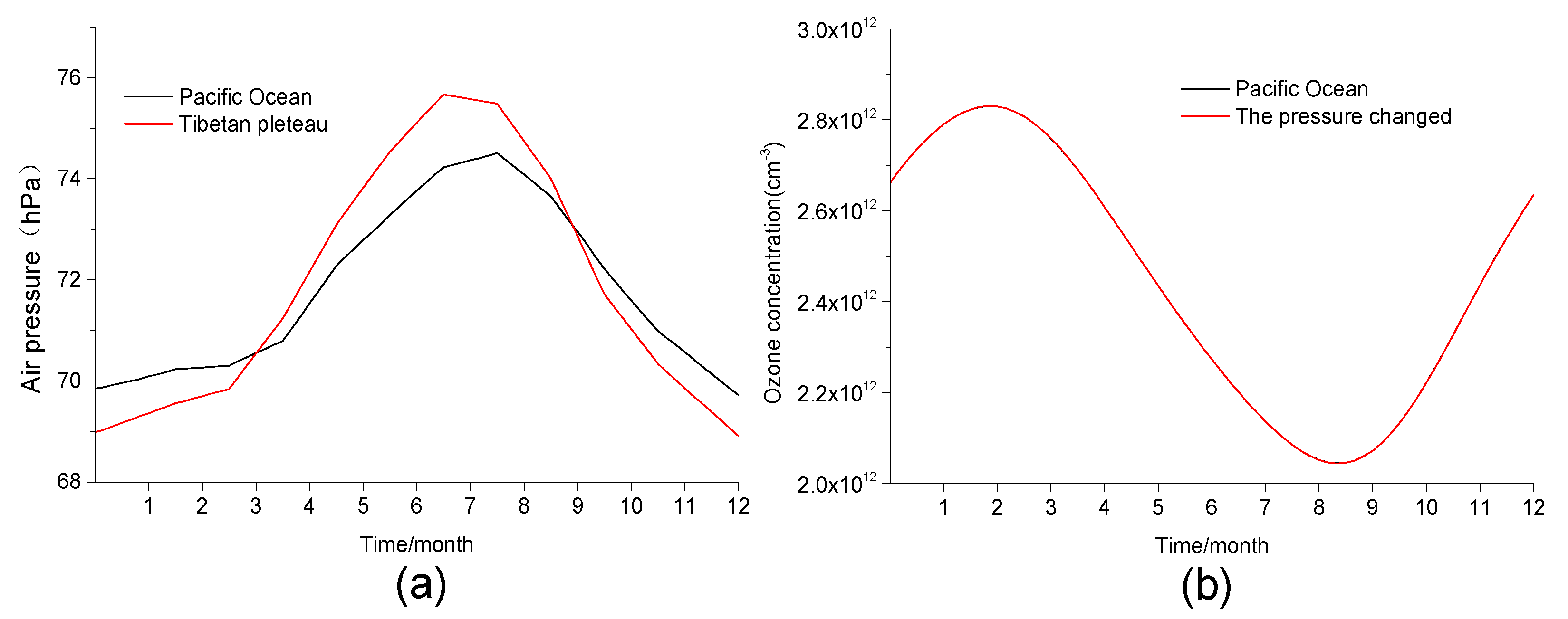
3.2. Influence of Temperature and Pressure

According to the analysis of SAGE II data, the pressure change over the Tibetan Plateau and the Pacific Ocean at the height of 18 km are slightly different. Although the pressure increases in summer and autumn and decreases in winter and spring at both regions, the pressure amplitude of the Tibetan Plateau is slightly larger than that over the Pacific Ocean, as shown in Figure 4a. In winter and spring, the pressure of the Tibetan Plateau is lower than outside the Tibetan Plateau region, but in summer and autumn, it is higher. The model we used contains only chemical processes and does not involve dynamic processes, such as air flow caused by changes in air pressure. It only considers that the air pressure affects the heterogeneous chemical reaction rate by affecting the content of sulfuric acid in the sulfuric acid droplets, thus affecting the chemical equilibrium.

The ozone response to changing pressure is shown in Figure 4b. It can be seen that the ozone concentration undergoes little change and that the two curves basically coincide. We calculated the effect of air pressure on the rate of a heterogeneous chemical reaction (N₂O₅ + H₂O→2 HNO₃) and found that the difference between the two places is approximately 10⁻¹⁷. This difference is so small that air pressure cannot have a significant effect on the ozone chemical equilibrium. Thus, the change in air pressure has little effect on the change in ozone concentration.

The temperature obtained from the analysis of SAGE II data is shown in Figure 5a. It can be seen that the temperature of the Tibetan Plateau in summer and autumn is significantly lower than during other seasons. In contrast, the summer–autumn temperature outside the Plateau is slightly higher than in other seasons. The largest difference between the two curves in summer and autumn is approximately 7 K. We only modified the temperature field on the basis of the original model and did not change the aerosol type. The simulation results are shown in Figure 5b,c,d.

Figure 5c shows that the concentration of ozone over the Tibetan Plateau is slightly higher than outside the Tibetan Plateau at the same latitude region from May to August, which basically corresponds to the period with a large temperature difference. However, the overall magnitude is 10¹⁰ cm⁻³, far less than 10¹² cm⁻³, and the influence ratio on the ozone valley is between −2% and 0; the lower the temperature, the higher the ozone concentration.

3.3. The Influence of Aerosols

In view of the analysis of satellite data, the aerosol area index in the nonpeak part (outside May to August), which is basically the same in both compared regions, is approximately 0.73 × 10⁻⁸ cm²/cm³. Therefore, we default to the fact that the aerosols in the nonpeak part of the Tibetan Plateau are the same as those of the Pacific Ocean region, that the type of aerosols is sulfuric acid droplets, and that the area index is 0.73 × 10⁻⁸ cm²/cm³, as shown in Figure 6a. Because there is no exact observation data of the composition and proportion of the ATAL aerosols, the peak of aerosol loading may due to any one of sulfuric acid droplets, solid sulfate, organic carbon, black carbon, sea salt, mineral dust, or a mixture in a certain proportion. To quantitatively estimate the possible effect of any of the heterogeneous chemical reactions on the ozone, we sequentially assume that the peak of the aerosol index is due to a single aerosol (as shown in Figure 6b) and then compare the variation in the ozone difference to determine the maximum influence of aerosols on the ozone valley.

When the increased summer aerosol loading is assumed to due to the sulfuric acid droplets (SLA), the model simulation shows that the ozone concentration is significantly decreased, as shown in the red lines in Figure 6b,c. The ozone concentration decreases more in summer and autumn and less in winter and spring. The overall magnitude can reach 1 × 10¹¹ cm⁻³, and the influence ratio relative to the ozone valley in summer (May to August) can reach approximately 5–17% (Figure 6d).

In the previous temperature field test (Figure 5b), the ozone concentration over the Tibetan Plateau is slightly higher than that in the same latitude region over the Pacific Ocean due to the temperature difference from May to August. After the single-peak distribution of the aerosol area index is added, the ozone concentration over the Tibetan Plateau is found to be far lower than that over the region outside the Plateau. Even when the aerosol area indices are equal, the ozone concentration over the Tibetan Plateau is still lower than that which it is over the Pacific Ocean, at the same latitude.

When only solid sulfate (Figure 6a) is considered, the ozone concentration also decreases to a certain extent, as shown by the blue line in Figure 6b and c. However, the ozone concentration decreases far less than when sulfuric acid droplets are considered, and the overall magnitude reaches only approximately 3 × 10¹⁰ cm⁻³. The trend is still more in summer and autumn and less in winter and spring. The influence ratio of the ozone valley in summer (May to August) can reach approximately 2–5%, as shown in Figure 6d.

When the aerosol peak (Figure 6a) is attributed to the organic carbon (OC), black carbon (BC), sea salt (SALT) or mineral dust (DUST), the model simulation shows that the range of the decrease in ozone concentration is basically the same and that the overall magnitude is approximately 8 × 10⁹ cm⁻³, among which the decrease caused by organic carbon is the lowest. From the perspective of seasonal change, the decrease is still more in summer and autumn and less in winter and spring. The influence ratios on the ozone valley are 0.6–1.8% for mineral dust, 0.6–1.6% for black carbon, 0.5–1.6% for sea salt and 0.5–1.5% for organic carbon (Figure 6d).

Figure 6c shows that the influence of the above aerosols on the variation in ozone concentration is greater in summer and autumn and smaller in winter and spring and that the peak value of the influence caused by aerosols slightly lags behind the peak value of the aerosol. Among the different types of aerosol, the sulfuric acid droplet aerosol influence on ozone is the largest, followed by solid sulfate, and there is no significant difference among the effects of black carbon, sea salt, mineral dust and organic carbon. The influence of sulfuric acid droplets is approximately 10 times that of organic carbon, black carbon, sea salt and mineral dust aerosols.

Figure 6b shows that the ozone concentration curve of the Tibetan Plateau is lower not only in summer and autumn but also in winter and spring. There is still a large gap between the ozone change curves of the Tibetan Plateau in Figure 6b and Figure 1. In summer and autumn, the observed value is far lower than the simulated value, which shows that the increased aerosol loading and initiated by it heterogeneous ozone loss is not the main cause of the ozone valley—it is only a part of it, and the main reason is the dynamic processes. In winter and spring, the observed value is higher than the simulation value, which shows that chemical factors are not the main factors that dominate the ozone over the Tibetan Plateau in winter and spring. For example, recent studies have shown that the ion–molecular reactions launched in the layer of secondary electrons—itself generated near the tropopause by galactic cosmic rays—could serve as a local source of ozone at middle to high latitudes [45].

4. Summary and Discussion

Using a box model of the heterogeneous chemical reactions of stratospheric ozone, this paper simulates the variation in ozone concentration with time at the altitude of 18 km between the Tibetan Plateau and a region outside the Tibetan Plateau at the same latitude. The preliminary results show that under the environmental conditions of the Tibetan Plateau, the changes in air pressure and temperature have little effect on the ozone valley; however, the lower the temperature is, the higher the ozone concentration. In other words, the temperature itself has a negative effect on the ozone chemistry.

From May to August, with the increase in aerosol area index, not only is the increase in ozone brought about by the low temperature in summer offset, but the ozone curve over the Tibetan Plateau is also lower than that over the same latitude region as a whole, which is much lower in summer. The sensitivity test shows that the heterogeneous chemical reactions on aerosols from May to August have an influence ratio of 0.5–17% on the ozone valley. In June, the maximum is approximately 5%. For the rest of the time, with the weakening of monsoon convection, the influence ratio of heterogeneous chemical reactions increases. For the whole summer, the possible influence ratios of aerosols on the ozone valley are as follows: 5–17% for sulfuric acid droplets, 2–5% for solid sulfate, 0.6–1.8% for mineral dust, 0.6–1.6% for black carbon, 0.5–1.6% for sea salt, and 0.5–1.6% for organic carbon. The decrease in ozone caused by heterogeneous chemical reactions on aerosols is greater in summer and autumn than in winter and spring.

It can be seen from the heterogeneous chemical reactions on the aerosol surface that organic carbon, black carbon and mineral dust mainly interfere with the chemical equilibrium of ozone through the “denitrification process”:

NO₂ + 0.5 × H₂O→0.5 HNO₃+0.5 HNO₂

(7)

NO₃ + H₂O→HNO₃ + OH

(8)

N₂O₅ + H₂O→2 HNO₃

(9)

Denitrification will significantly reduce the formation of storage molecules of chlorides and bromides, thus increasing the amount of active ClO and BrO (shown in Figure 7) and increasing the destruction of ozone. However, sulfuric acid droplets and solid sulfate will interfere with the ozone equilibrium, not only through the denitrification process, but also through the following reactions:

HOCl + HCl→Cl₂ + H₂O

(10)

ClONO₂ + H₂O→HOCl + HNO₃

(11)

ClONO₂ + HCl→Cl₂ + HNO₃

(12)

These reactions transform the reservoir molecules, such as ClONO₂ and HCl, into HOCl and Cl₂, which are easier to photo dissociate. This process is generally called “chlorine activation”. After activation, the degradation cycles of ClONO₂ and HOCl form ClO and Cl to destroy ozone more effectively.

In addition, through the reactions

HOCl + HBr→BrCl + H₂O

(13)

HOBr + HCl→BrCl + H₂O

(14)

HOBr + HBr→Br₂ + H₂O

(15)

BrONO₂ + H₂O→HOBr + HNO₃

(16)

BrONO₂ + HCl→BrCl + HNO₃

(17)

the dominant product BrCl is finally formed (shown in Figure 7), which is a process called “bromine activation”. Bromide is a more effective ozone-depleting substance. With the continuous increase in emissions from human activities, the influence of heterogeneous chemical reactions on anthropogenic aerosols on the summer ozone valley of the Tibetan Plateau will probably increase.

At the same time, the main absorption wavelength of ClONO₂ is 196–432.5 nm, and that of NO₃ is 472.5–627.5 nm. The wavelengths of solar radiation at the height of 18 km are mainly between 200–735 nm, so the photolysis of ClONO₂ and NO₃ in the daytime will lead to more intense ozone destruction.

ClO + NO₂ + M→ClONO₂ + M

(18)

ClONO₂ + hγ₁→Cl + NO₃

(19)

Cl + O₃→ClO + O₂

(20)

NO₃ + hγ₂→NO + O₂

(21)

NO + O₃→NO₂ + O₂

(22)

2O₃ + hγ₁ + hγ₂→3O₂

(23)

These results show that the effects of heterogeneous chemical reactions on ozone are closely related to the types and coefficients of heterogeneous chemical reactions initiated on the aerosols surface. For example, the number of heterogeneous chemical reactions on sulfuric acid droplets is greater than that on the other types of aerosols. However, due to the lack of in situ measurements of the chemical composition of ATAL aerosols, there is still definitely great controversy regarding the source and composition of the ATAL. Therefore, further studies are needed to determine the influence of heterogeneous chemical reactions of aerosols on ozone.

References

1. Farman, J.C.; Gardiner, B.G.; Shanklin, J.D. Large losses of total ozone in Antarctica reveal seasonal ClOx/NOx interaction. Nature 1985, 315, 207–210. [Google Scholar] [CrossRef]
2. Lefèvre, F.; Figarol, F.; Carslaw, K.S.; Peter, T. The 1997 Arctic Ozone depletion quantified from three-dimensional model simulations. Geophys. Res. Lett. 1998, 25, 2425–2428. [Google Scholar] [CrossRef]
3. Zhou, X.; Luo, C.; Li, W.; Shi, J. The changes of total ozone in China and low value ozone center of Tibetan Plateau. Chinese Sci. Bull. 1995, 40, 1396–1398. [Google Scholar]
4. Fu, C.; Li, W.; Zhou, X. A simulated experiment on the formation of the ozone valley in summer over the Tibetan Plateau. In Changes of Atmospheric Ozone in China and Its Influence on Climate and Environment; China Meteorological Press: Beijing, China, 1997. (In Chinese) [Google Scholar]
5. Tian, W.; Chipperfield, M.; Huang, Q. Effects of the Tibetan Plateau on total column ozone distribution. Tellus 2008, 60B, 622–635. [Google Scholar] [CrossRef]
6. Bian, J. Recent advances in the study of atmospheric vertical structures in upper troposphere and lower stratosphere. Adv. Earth Sci. 2009, 24, 262–271. [Google Scholar]
7. Guo, D.; Zhou, X.; Liu, Y.; Li, W.; Wang, P. The dynamic effects of the South Asian high on the ozone valley over the Tibetan Plateau. Acta Meteorol. Sinica. 2012, 70, 1302–1311. (In Chinese) [Google Scholar] [CrossRef]
8. Xu, P.; Tian, W.; Zhang, J.; Luo, J.; Huang, Q.; Zhang, J. A simulation study of the transport of the stratospheric ozone to the troposphere over the northwest side of the Tibetan Plateau in spring. Acta Meteorol. Sinica 2015, 73, 529–545. (In Chinese) [Google Scholar]
9. Liu, Y.; Li, W.L.; Zhou, X.J.; He, J. Mechanism of formation of the Ozone Valley over the Tibetan Plateau in summer transport and chemical process of ozone. Adv. Atmos. Sci. 2003, 20, 103–109. [Google Scholar] [CrossRef]
10. Randel, W.J.; Park, M. Deep convective influence on the Asian summer monsoon anticyclone and associated tracer variability observed with Atmospheric Infrared Sounder (AIRS). J. Geophys. Res. 2006, 111, D12314. [Google Scholar] [CrossRef]
11. Randel, W.J.; Park, M.; Emmons, L.; Kinnison, D.; Bernath, P.; Walker, K.A.; Boone, C.; Pumphrey, H. Asian monsoon transport of pollution to the stratosphere. Science 2010, 328, 611–613. [Google Scholar] [CrossRef] [Green Version]
12. Park, M.; Randel, W.J.; Gettelman, A.; Massie, S.T.; Jiang, J.H. Transport above the Asian summer monsoon anticyclone inferred from Aura Microwave Limb Sounder tracers. J. Geophys. Res. 2007, 112, D16309. [Google Scholar] [CrossRef] [Green Version]
13. Park, M.; Randel, W.J.; Emmons, L.K.; Livesey, N.J. Transport pathways of carbon monoxide in the Asian summer monsoon diagnosed from model of ozone and related tracers (MOZART). J. Geophys. Res. 2009, 114, D08303. [Google Scholar] [CrossRef] [Green Version]
14. Bian, J.; Yan, R.; Chen, H. Tropospheric pollutant transport to the stratosphere by Asian summer monsoon. Chinese J. Atmos. Sci. 2011, 35, 897–902. (In Chinese) [Google Scholar]
15. Solomon, S. Stratospheric ozone depletion: A review of concepts and history. Rev. Geophys. 1999, 37, 275–316. [Google Scholar] [CrossRef]
16. Vernier, J.P.; Thomason, L.W.; Kar, J. CALIPSO detection of an Asian tropopause aerosol layer. Geophys. Res. Lett. 2011, 38, 1451–1453. [Google Scholar] [CrossRef] [Green Version]
17. Thomason, L.W.; Vernier, J.P. Improved SAGE II cloud/aerosol categorization and observations of the Asian tropopause aerosol layer: 1989–2005. Atmos. Chem. Phys. 2013, 13, 4605–4616. [Google Scholar] [CrossRef] [Green Version]
18. Junge, C.E.; Chagnon, C.W.; Manson, J.E. Stratospheric aerosols. J. Meteorol. 1961, 18, 81–108. [Google Scholar] [CrossRef]
19. Li, W.; Yu, S. A numerical simulation of the Spatial-temporal distribution of aerosols over the Tibetan Plateau and their radiative forcing and climatic effects. Sci. China (D Ser.) 2001, B12, 300–307. (In Chinese) [Google Scholar]
20. Zhou, R.; Chen, Y.; Bi, Y.; Yi, M. Aerosol distribution over the Tibetan Plateau and its relationship with ozone. Plateau Meteorol. 2008, 27, 500–508. (In Chinese) [Google Scholar]
21. Liu, Y.; Li, W.; Zhou, X. A possible effect of heterogeneous reactions on the formation of the ozone valley over the Tibetan Plateau. Acta Meteorol. Sinica 2010, 68, 836–846. (In Chinese) [Google Scholar]
22. Thomason, L.W.; Bedka, K.M. Increase in upper tropospheric and lower stratospheric aerosol levels and its potential connection with Asian pollution. J. Geophys. Res. Atmos. 2015, 120, 1608–1619. [Google Scholar]
23. Margaret, A.T. Polar clouds and Sulfate Aerosols. Science 1996, 272, 1597. [Google Scholar]
24. Lowe, D.; Mackenzie, A.R. Polar stratospheric cloud microphysics and chemistry. J. Atmos. Sol.-Terr. Phy. 2008, 70, 13–40. [Google Scholar] [CrossRef] [Green Version]
25. Mauldin, L.E.; Zaun, N.H.; McCormick, M.P.; Guy, J.H.; Vaughn, W.R. Stratospheric aerosol and gase experiment II instrument: A functional description. Opt. Eng. 1985, 24, 242307. [Google Scholar] [CrossRef]
26. Chu, W.P.; McCormick, M.P.; Lenoble, J.; Brogniez, C.; Pruvost, P. SAGE II inversion algorithm. J. Geophys. Res. 1989, 94, 8339–8351. [Google Scholar] [CrossRef]
27. Thomason, L.W.; Poole, L.R.; Randall, C.E. SAGE III aerosol extinction validation in the Arctic winter: Comparisons with SAGE II and POAM III. Atmos. Chem. Phys. 2007, 7, 1423–1433. [Google Scholar] [CrossRef] [Green Version]
28. Steinbrecht, W.; Claude, H.; Köhler, U.; Hoinka, K.P. Correlations between tropopause height and total ozone: Implications for long-term changes. J. Geophys. Res. 1998, 103, 19183–19192. [Google Scholar] [CrossRef]
29. Yang, P.; Brasseur, G. Dynamics of the oxygen-hydrogen system in the mesosphere: 1. Photochemical equilibria and catastrophe. J. Geophys. Res. 1994, 99, 20955–20965. [Google Scholar] [CrossRef]
30. Wang, G.; Yang, P. On the Nonlinear response of lower stratosphere ozone to NOX and ClOX perturbations. Chinese J. Geophy. 2007, 50, 51–57. (In Chinese) [Google Scholar] [CrossRef]
31. Yan, J.; Jin, L.; Wang, G. A Study of the mechanism of nonlinear responses in stratospheric ozone. Climat. Env. Res. 2012, 17, 639–645. (In Chinese) [Google Scholar]
32. Yu, P.; Toon, O.B.; Neely, R.R.; Martinsson, B.G.; Brenninkmeijer, C.A.M. Composition and physical properties of the Asian tropopause aerosol layer and the North American tropospheric aerosol layer. Geophys. Res. Lett. 2015, 42, 2540–2546. [Google Scholar] [CrossRef]
33. Gu, Y.; Liao, H.; Bian, J. Summertime nitrate aerosol in the upper troposphere and lower stratosphere over the Tibetan Plateau and the South Asian summer monsoon region. Atmos. Chem. Phys. 2016, 15, 32049–32099. [Google Scholar] [CrossRef]
34. Carslaw, K.S.; Luo, B.P.; Clegg, S.L.; Peter, T.; Brimblecombe, P.; Crutzen, P.J. Stratospheric aerosol growth and HNO3 gas phase depletion from coupled HNO3 and water uptake by liquid particles. Geophys. Res. Lett. 1994, 21, 2479–2482. [Google Scholar] [CrossRef]
35. Carslaw, K.S.; Luo, B.P.; Peter, T. An analytic expression for the composition of aqueous HNO3-H2SO4 stratospheric aerosols including gas phase removal of HNO3. Geophys. Res. Lett. 1995, 22, 1877–1880. [Google Scholar] [CrossRef]
36. Carslaw, K.S.; Peter, T.; Clegg, S.L. Modeling the composition of liquid stratospheric aerosols. Rev. Geophys. 1997, 35, 125–154. [Google Scholar] [CrossRef]
37. Yu, P.; Rosenlof, K.H.; Liu, S.; Telg, H.; Thornberry, T.D.; Rollins, A.W.; Portmann, R.W.; Bai, Z.; Ray, E.A.; Duan, Y.; et al. Efficient transport of tropospheric aerosol into the stratosphere via the Asian summer monsoon anticyclone. P. Natl. Acad. Sci. 2017, 114, 6972–6977. [Google Scholar] [CrossRef] [Green Version]
38. Kirner, O.; Ruhnke, R.; Buchholz-Dietsch, J.; Jökel, P.; Brühl, C.; Steil, B. Simulation of polar stratospheric clouds in the chemistry-climate-model EMAC via the submodel PSC. Geosci. Model Dev. Discuss. 3 2010, 2071–2108. [Google Scholar] [CrossRef]
39. Burkholder, J.B.; Sander, S.P.; Abbatt, J.; Barker, J.R.; Huie, R.E.; Kolb, C.E.; KuryloM, J.; Orkin, V.L.; Wilmouth, D.M.; Wine, P.H. Chemical kinetics and photochemical data for use in atmospheric studies; Evaluation No.18, JPL Publication 15-10; Jet Propulsion Laboratory: Pasadena, CA, USA, 2015. [Google Scholar] [CrossRef]
40. Zhou, R.; Chen, Y. Ozone variations over the Tibetan and Iranian Plateaus and their relationship with the South Asia High. J. Univ. Sci. Tech. Chin. 2005, 35, 899–908. (In Chinese) [Google Scholar]
41. Vernier, J.P.; Pommereau, J.P.; Garnier, A.; Pelon, J.; Larsen, N.; Nielsen, J.; Christensen, T.; Cairo, F.; Thomason, L.W.; Leblanc, T.; et al. Tropical stratospheric aerosol layer from CALIPSO lidar observations. J. Geophys. Res. 2009, 114, D00H10. [Google Scholar] [CrossRef] [Green Version]
42. Bourgeois, Q.; Bey, I.; Stier, P. A permanent aerosol layer at the tropical tropopause layer driven by the intertropical convergence zone. Atmos. Chem. Phys. Discuss. 2012, 12, 2863–2889. [Google Scholar] [CrossRef]
43. He, Q.; Li, C.; Ma, J.; Wang, H.; Yan, X.; Lu, J.; Liang, Z.; Qi, G. Lidar-observed enhancement of aerosols in the upper troposphere and lower stratosphere over the Tibetan Plateau induced by the Nabro volcano eruption. Atmos. Chem. Phys. 2014, 14, 11687–11696. [Google Scholar] [CrossRef] [Green Version]
44. Orlando, J.; Brasseur, G.; Tyndall, G.S. Atmospheric Chemistry and Global Change; Oxford University Press: Oxford, UK, 1999. [Google Scholar]
45. Kilifarska, N.A. Hemispherical asymmetry of the lower stratospheric O3 response to galactic cosmic rays forcing. ACS Earth Space Chem. 2017, 1, 80–88. [Google Scholar] [CrossRef]
Figure 1. Monthly mean variation curve of ozone number concentration at 18 km observed by satellite (black: the Pacific Ocean region (25–40° N, 140–180° E); red: the Tibetan Plateau (25–40° N, 70–110° E); blue: the quantitative difference between the preceding two curves (PO-TP)).
Atmosphere 11 00138 g001
Figure 2. Changes in air pressure (a), temperature (b) and aerosol area index (c) with time at the altitude of 18 km in the lower stratosphere observed by SAGE II (black: the Pacific Ocean region (25–40° N, 140–180° E); red: the Tibetan Plateau (25–40° N, 70–110° E)).
Atmosphere 11 00138 g002
Figure 3. Model simulation and satellite observation of ozone variation at 18 km altitude over the Pacific Ocean (25–40° N, 140–180° E) (The scattered points are the observation results, and the solid line shows the simulation results).
Atmosphere 11 00138 g003
Figure 4. The results of air pressure changes, (a) time-dependent variations in air pressure in the two regions; (b) simulated comparison of the ozone number concentrations in the two regions.
Atmosphere 11 00138 g004
Figure 5. The results of air temperature changes (a) time-dependent variations in air temperature in the two regions; (b) simulated comparison of the ozone number concentrations in the two regions; (c) difference in simulated ozone number concentration between the two regions; (d) ratio of the ozone simulation difference to the observed difference after changing temperature.
Atmosphere 11 00138 g005
Figure 6. Similar to Figure 5, the modeled ozone response to aerosol changes (SLA is sulfuric acid droplets; SAT is solid sulfate; OC is organic carbon; BC is black carbon; SALT is sea salt; DUST is mineral dust).
Atmosphere 11 00138 g006
Figure 7. Changes in NOx/Clx/Brx over time over the Tibetan Plateau.
Atmosphere 11 00138 g007