Article

Correction of Light Scattering-Based Total Suspended Particulate Measurements through Machine Learning

1
China-UK Low Carbon College, Shanghai Jiao Tong University, Shanghai 200240, China
2
Shanghai Eureka Environmental Protection Hi-tech., Ltd., Shanghai 200090, China
3
School of Environmental Science and Engineering, Shanghai Jiao Tong University, Shanghai 200240, China
4
Division of Atmospheric Sciences, Desert Research Institute, 2215 Raggio Parkway, Reno, NV 89512, USA
5
Shanghai Environmental Monitoring Center, Shanghai 200235, China
*
Author to whom correspondence should be addressed.
Atmosphere 2020, 11(2), 139; https://doi.org/10.3390/atmos11020139
Submission received: 17 November 2019 / Revised: 23 January 2020 / Accepted: 24 January 2020 / Published: 26 January 2020
(This article belongs to the Section Atmospheric Techniques, Instruments, and Modeling)

Abstract

:
Instruments based on light scattering used to measure total suspended particulate (TSP) concentrations have the advantages of fast response, small size, and low cost compared to the gravimetric reference method. However, the relationship between scattering intensity and TSP mass concentration varies nonlinearly with both environmental conditions and particle properties, making it difficult to make corrections. This study applied four machine learning models (support vector machines, random forest, gradient boosting regression trees, and an artificial neural network) to correct scattering measurements for TSP mass concentrations. A total of 1141 hourly records of collocated gravimetric and light scattering measurements taken at 17 urban sites in Shanghai, China were used for model training and validation. All four machine learning models improved the linear regressions between scattering and gravimetric mass by increasing slopes from 0.4 to 0.9–1.1 and coefficients of determination from 0.1 to 0.8–0.9. Partial dependence plots indicate that TSP concentrations determined by light scattering instruments increased continuously in the PM2.5 concentration range of ~0–80 µg/m3; however, they leveled off above PM10 and TSP concentrations of ~60 and 200 µg/m3, respectively. The TSP mass concentrations determined by scattering showed an exponential growth after relative humidity exceeded 70%, in agreement with previous studies on the hygroscopic growth of fine particles. This study demonstrates that machine learning models can effectively improve the correlation between light scattering measurements and TSP mass concentrations with filter-based methods. Interpretation analysis further provides scientific insights into the major factors (e.g., hygroscopic growth) that cause scattering measurements to deviate from TSP mass concentrations besides other factors like fluctuation of mass density and refractive index.

1. Introduction

Total suspended particulate (TSP) generally refers to particulate matter suspended in air with an aerodynamic equivalent diameter of less than 100 µm. Ambient particulate matter (PM) measurements are obtained using an offline manual method and an online automatic method. Offline methods usually refer to integrated filter sampling followed by gravimetric weighing, which is regarded as the reference method [1]. Filter sampling has poor time resolution (typically 24 hours) and the data are not available for several days while the filters are equilibrated and weighed in a laboratory. Online automatic methods mainly include Tapered Element Oscillating Microbalance (TEOM), β-ray attenuation, and light scattering. The TEOM method is based on the principle of frequency changes when the oscillation element is loaded with particles, while the β-ray method estimates PM mass loading based on β-ray energy attenuation across a PM loaded filter [2,3,4]. These two methods are usually accurate and the time resolution can be as high as a few minutes; however, the large size and high cost of these instruments limit their wide application. Light scattering methods estimate PM mass from the particle light scattering intensity [5,6,7]. Due to their fast response time, high sensitivity, and low cost, light scattering instruments are widely used as portable real-time particle monitors.
Despite the many advantages of the light scattering method, it does not measure PM mass based on first principles (gravimetry) and it suffers from limited accuracy and stability especially for low-cost sensors with small sampling volumes. The relationship between scattering intensity and PM mass concentration depends on environmental conditions and particle properties, such as relative humidity (RH), particle chemical composition, refractive index, size distribution, and density [7,8,9]. Light scattering instruments are only sensitive to particles larger than ~100 nm; therefore, they underestimate the mass concentrations of nanoparticles. However, nanoparticles are expected to contribute only a small fraction of TSP mass in a typical ambient environment. Previous studies have shown significant growth in atmospheric aerosols at RH higher than 70%, which enhances light scattering and causes overestimation of PM mass (as compared to gravimetry) [8,9]. It is critical to correct these dependencies when converting light scattering measurements by using low-cost instruments to PM mass concentrations.
Several studies have shown that machine learning algorithms can be effective for correcting atmospheric measurements. Suleiman et al. used Artificial Neural Networks (ANN), Boosted Regression Trees (BRT), and Support Vector Machines (SVM) to correct the traffic-related PM10 and PM2.5 concentrations at 19 air quality monitoring sites in urban London [9]. Zou et al. proposed a radial basis function neural network to predict PM2.5 concentrations in Texas, USA through meteorological factors and land-related factors [10]. Sayegh et al. used BRT to predict NOX concentrations based on the hourly concentration, traffic, and meteorological data [11]. Most past studies focused on correcting the concentrations of PM2.5, PM10, or gaseous pollutants such as nitrogen dioxide and carbon dioxide. In contrast, not much research on TSP (≤100 μm) correction has been reported. Due to its wide size range, TSP has more diverse particle physical and chemical properties, which also lead to more complicated hygroscopic effects, making the correction of TSP mass concentrations reported by light scattering instrument more challenging.
This study aims to develop and validate machine learning models to correct light scattering instruments that report TSP mass concentrations. Four models were trained and tested on TSP datasets from collocated light scattering and filter measurements in Shanghai, China. TSP is one of the main pollutants in Shanghai, particularly in locations close to construction sites, storage piles, and busy roads. Partial dependence plots were used to interpret factors (e.g., hygroscopic growth) affecting the model outputs.

2. Materials and Methodology

2.1. Monitoring Instruments and Data Collection

TSP data were collected at 52 monitoring sites in the urban area of Shanghai, the largest megacity of China, over the period from June 6, 2017 to September 20, 2018. Each site had collocated TSP mass concentration measurements determined by online light scattering and offline filter measurements in addition to meteorological parameters. Real-time TSP mass concentrations were measured by a light scattering dust monitor (Model CEL-712 Microdust Pro, Casella, Bedford, UK; referred to as Casella in this paper) calibrated by the manufacturer using Arizona road dust (ISO 12103-1 test dust) [12]. The instrument intake flow is 1.7 L/min. The Casella uses near forward light scattering to reduce the influence of particle refractive indices on the scattering intensity [13]. In this study, the TSP device measures traffic emissions. For TSP collection we used Laoying 2030 medium flow rate intelligent TSP samplers, following the operation and QA/QC procedures specified in the China national standards GB/T15432-1995. For gravimetry analyses, we used a Mettler-Toledo MS105DU semi-micro balance with an accuracy of 0.01 mg. Prior to weighing, filters were equilibrated in a chamber with controlled temperature (25 °C) and RH (50%) for at least 24 hrs. Each filter was weighed twice and if the relative difference of the two weights exceeded 5%, the filter was weighed a third time. The average concentrations of the two weights with a difference <5% are reported. The ambient temperature and RH during the sampling period were recorded by a Hengxin AZ-8809 High Precision Humidity Temperature Recorder at each sampling site. Furthermore, hourly mass concentrations of ambient PM2.5, PM10, SO2, NO2, CO, and O3 were measured at the Caoxi Traffic Site with the most abundant data records. For the remaining sits, they were obtained from nearby sites of the national official monitoring network in Shanghai and used as the input indices for the prediction models. To ensure spatial consistency, 17 TSP monitoring sites and 7 national monitoring stations in urban Shanghai with geographical distances between 0.63 and 3.5 km were identified and selected (shown in Figure 1) for this study. The information about TSP sites and nearby national monitoring stations are shown in Table 1. This selection resulted in a total of 1141 hourly records in the monitoring datasets that were used for the model development and validation. The parameters used as model predictors and measurement instruments are listed in Table 2. The hourly criteria pollutant concentrations, temperature, and humidity will help resolve the potentially confounding influences on the accuracy of the Casella TSP measurements.

2.2. Model Development and Data Preparation

Four supervised machine learning models (support vector machines (SVM), random forest (RF), gradient boosting regression trees (GBRT), and artificial neural networks (ANN)) were used in this study to correct the raw TSP concentration outputs by the Casella dust monitors. SVM is a powerful machine learning model that can perform linear or nonlinear classification, regression, and outlier detection tasks [14,15]. RF is a branch of ensemble learning algorithms that is composed of multiple decision trees. Ensemble learning includes Boosting and Bagging methods. RF is an extension of Bagging [16,17,18], while GBRT is one of the Boosting algorithms. Predictors are gradually added in the training process, each of which corrects its former predictor [19]. ANN is a multi-layer network consisting of an input layer, multiple hidden layers, and an output layer. Each layer can be regarded as a logistic regression mode. The backpropagation algorithm is used based on the gradient descent strategy.
The SVM parameters set during the training were the kernel type, cost and sigma parameters. In this study, we used a Radial Basis Function (RBF) kernel to train the SVM model. The cost and sigma values were 1 and 0.1, respectively. The model parameters for an RF model are the number of trees, minimum samples split and bootstrap. We selected 500 estimators (trees) to train the RF and set the minimum samples split to 2 and bootstrap to true. For the GBRT model, we also selected 500 trees for the training and the learning rate was 0.01. The ANN model in this study contained two hidden layers and 100 hidden neurons in each layer, the activation function was the Rectified Linear Unit (ReLU) function, and the maximum number of iterations was set to 400.
The input variables included the hourly TSP mass concentrations from the Casella raw readings based on light scattering obtained at each site, criteria pollutant concentrations from the nearest national monitoring stations (PM2.5, PM10, SO2, NO2, CO, and O3), ambient temperature, and RH (Table 2). The unique output variable is hourly gravimetric TSP mass concentration at the same time as the Casella sampling. The Casella instrument monitors TSP concentrations based on light scattering continuously and hourly averages of raw readings were used in the data analysis. We put the training dataset (80% of total the records, randomly selected) into the four machine learning models to reconstruct the non-linear relationship between the input and output variables. A 5-fold cross-validation as a resampling method was used to develop the models. After model training, the remaining 20% of the records were used to validate the reconstructed models. Due to the significant discrepancy of data volume (from to records) between different measurement sites in this study, it is unfair and improper to divide the training and testing datasets by station level, although the splitting by station level seems more reasonable and could avoid the problem of information leakage. Python programming language, pandas, and Scikit-Learn packages were used to train and validate the models.

3. Results and Discussion

3.1. Performance of Machine Learning Models in Predicting TSP

The performance of the models was evaluated using various metrics including the Mean Square Error (MSE), Root Mean Squared Error (RMSE), Mean Absolute Error (MAE), and coefficient of determination (R2). The mean/standard deviation R2 results of 5-fold cross-validation were 0.75/0.07 for SVM, 0.76/0.02 for GBRT, 0.78/0.03 for RF, and 0.81/0.04 for ANN. The cross-validation results show that ANN had the best performance while the SVM model performed poorer than the other three models.
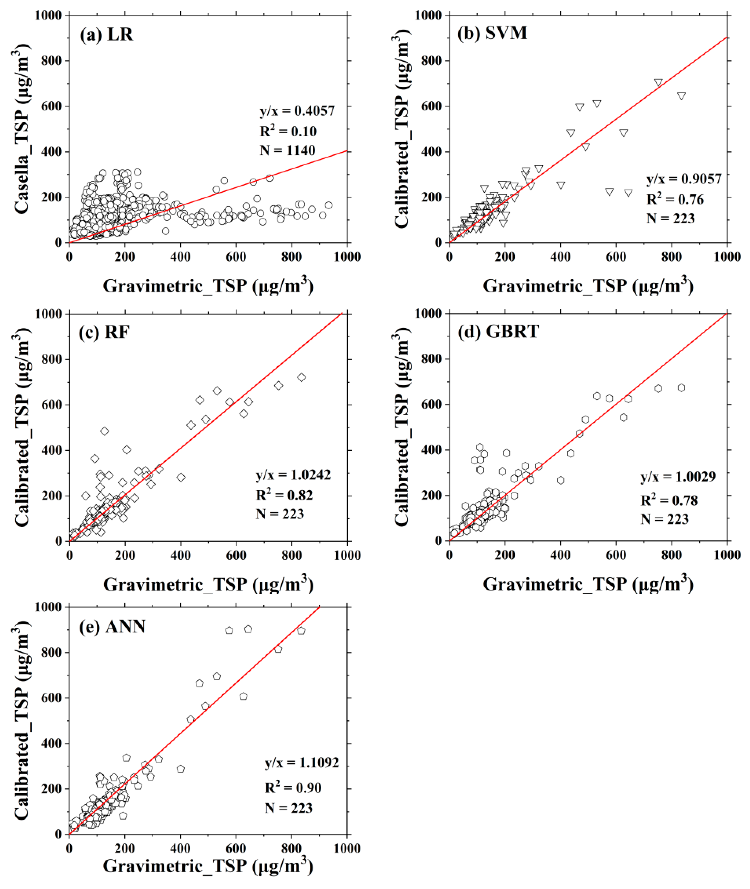
Figure 2 shows the performance of the four trained machine learning models in predicting TSP, and the overall predicting performance is summarized in Table 3. Figure 2a shows that the Casella raw TSP reading based on light scattering were poorly correlated with gravimetric TSP across the entire concentration range (~0–1000 µg/m3), with a low linear regression slope of 0.41 and R2 of only 0.10. At high concentrations (≳400 µg/m3), the Casella readings did not increase with the gravimetric concentrations. Figure 2b–e shows that the machine learning models significantly improved the agreement between the corrected Casella and reference TSP concentrations for the 223 validation dataset. The linear regression slope increased from the original 0.41 to 0.91–1.11 and R2 increased from 0.10 to 0.76–0.90. Interestingly, all four models were able to correct those high concentrations data points (≳400 µg/m3) for which the Casella seemed saturated. Among the four models, RF and GBRT had slopes (1.02 and 1.00, respectively) closer to 1.00 than did SVM and ANN (0.91 and 1.11, respectively). However, both RF and GBRT had a small group of datasets deviating from the regression lines with corrected concentrations being higher than the gravimetric concentrations at concentrations < 200 µg/m3, resulting in lower R2. On the other hand, this group of “outliers” were corrected successfully by ANN, resulting in a high R2 of 0.9. We note that the reasonable performance of the ANN was achieved by using only two hidden layers in this study, implying that a very complex and deep neural network is not always necessary. The SVM model had a few outliers with corrected concentrations being lower than the gravimetric mass concentrations, partially contributing to the lower slope and R2.
Similar improvement in correcting raw data by machine learning models have been reported in several recent studies. Suleiman et al. developed and applied three machine learning models (SVM, BRT, and ANN) to predict the roadside PM10 and PM2.5 concentrations in London. The models performed well: ~95% of predicted values were within a factor of 2 of the observations and the R2 values were in the range of 0.62–0.77 [9]. Similar to the finding of our study, Suleiman showed that the ANN and BRT models performed better than the SVM model, especially for PM10 prediction. It was speculated that the SVM over-fitted the PM10 data and failed to generalize the performance gained during training. Zimmerman et al. used an RF model to correct the low-cost air quality sensors that measured CO, NO2, O3, and CO2 [20]. The RF model consistently outperformed laboratory calibration and multiple linear regression corrections. The RF-corrected sensor readings had relative errors of <5% for CO2, 10%–15% for CO and O3, and ~30% for NO2. When the RF-corrected sensor readings were regressed against reference monitors for ambient concentrations measured in Pittsburgh, Pennsylvania, USA, the slopes of the linear regression lines for CO, NO2, and O3 were 0.86 ± 0.09, 0.64 ± 0.11, and 0.82 ± 0.05, respectively, and the R2 values were 0.91, 0.67, and 0.86, respectively. Brokamp et al. used RF to predict PM2.5 concentrations with a 1 km × 1 km spatial resolution from aerosol optical density and supplemental measurement data. The modeled data had an RMSE of 2.22 µg/m3 and R2 of 0.91 when compared with reference PM2.5 concentrations [18].
Figure 3 illustrates three examples of time series data obtained from the CaoXi road site, which had the most complete data capture among all 52 TSP monitoring sites. The overall information is shown in Table 4. During the first time period of 15 June 2017 to 22 June 2017, the average TSP concentrations were 92.28 μg/m3 and 132.22 μg/m3 from the Casella raw reading and gravimetric measurement, respectively. The gravimetric over Casella TSP concentration ratios varied from 0.30 to 3.35. The average TSP concentrations by the four machine learning models (SVM, RF, GBRT, ANN) were 132.85, 133.15, 132.53, and 134.04 μg/m3, deviating from the gravimetric mass by less than 1.5%. During the second period of 23 February 2018 to 27 February 2018, the average TSP concentrations were 108.10 μg/m3 and 121.15 μg/m3 from the Casella raw reading and gravimetric measurement, respectively; the average TSP concentrations by the four machine learning models (SVM, RF, GBRT, ANN) were 114.96, 119.92, 120.71 and 119.83 μg/m3, respectively. During the third time period of June 15, 2018 to June 30, 2018, the raw TSP concentrations by the Casella were as high as 236.4–242.8 μg/m3 on June 20, 2018, while the gravimetric TSP concentrations were only 65.3–89.6 μg/m3. The RH values on that day were as high as 90.0%–93.4%. The average TSP concentrations were 94.53 μg/m3 and 107.73 μg/m3 from the Casella raw reading and gravimetric measurements, respectively. The average TSP concentrations by the four machine learning models (SVM, RF, GBRT, ANN) were 104.82–107.96 μg/m3. Overall, all four machine learning methods can fit the result of the gravimetric method. The SVM model performed poorer than the other three models.
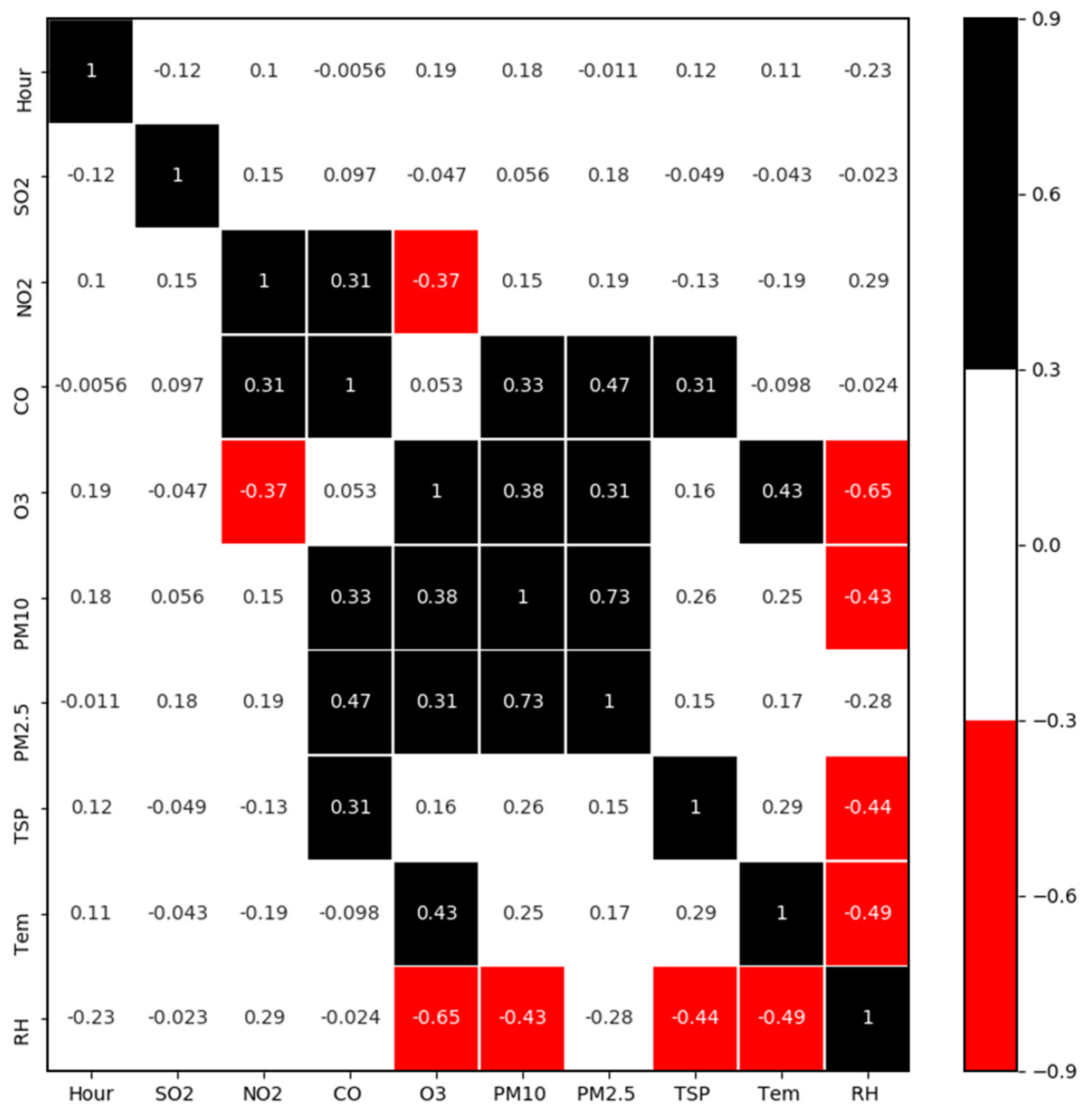
The random forest method provides a very convenient tool for importance analysis. It can estimate the importance or amount of contribution by a feature by calculating the average depth of a feature on all trees in the forest. Figure 4 plots the feature importance of different factors on Casella readings. It can be seen that PM2.5, RH, TSP, and PM10 are the top four factors influencing TSP concentration determined by a Casella monitor, which should be the focuses for follow-up analysis. Among the gaseous pollutants, CO and O3 relatively higher influences as compared to SO2 and NO2. Compared with relative humidity, the temperature had a minor direct impact on the measurement results. Temperature affects the gas-particle partitioning of semi-volatile species, such as nitrate and some organics. However, the mass contribution of these species to TSP is probably low and their evaporation is also affected by RH, leading to a lower influence by temperature. As an additional method to understand factor importance. We did an ablation study for the other three models. We calculated the average R2 and RMSE over 5-folds cross-validation when we exclude each factor. The results of the difference from all features are shown in Figure 4b,c. The three most impactful features were PM2.5, RH, and TSP. Four models have almost the same results, which means the results are scientific. We used a correlation analysis method to analyze the Pearson correlation coefficient between features (shown in Figure 5). The closer the value is to 1, the higher the correlation is. The result shows that the relationship between PM2.5 and PM10 is very close, which has a correlation coefficient of 7.3. RH has a negative correlation with most features (O3, PM2.5, PM10, TSP, Tem). The correlation coefficient between O3 and NO2 is −0.37.

3.2. Partial Dependence of Influencing Factors

As a model-agnostic interpretation method, the Partial Dependence Plot (PDP) charts were used to analyze the influence of different features on the light scattering instrument [21]. The partial dependence was estimated by calculating averages in the training data, also known as the Monte Carlo method:
f ^ X s ( X s ) = 1 n i = 1 n f ^ ( X s , X c ( i ) ) ,
The X s are the features for which the partial dependence function should be plotted and X c are the other features used in the machine learning model f ^ . The partial function relates the value(s) of features S to the average marginal effect on the prediction.
PDPs were generated for RF, GBRT, and ANN. This analysis was not conducted for SVM as it had poorer performances than the other three models and its PDPs had larger biases. Other methods, such as ICE (Individual Conditional Expectation) and ALE (Accumulated Local Effects) plots, are also available to reveal how features affect machine learning model predictions. These methods will be explored in future studies. This study focuses on assessing the different influences on light scattering monitors so we exchanged the input variable “Casella raw TSP readings” and output variable “Gravimetric TSP results” to rebuild the model.
Both one-way and two-way plots were used to show the effects of the four variables: PM2.5, PM10, gravimetric TSP concentrations, and RH on the Casella raw TSP readings. The scattering hygroscopic curves, which show how RH influences light scattering-based TSP concentrations, were further investigated. The scattering hygroscopic factor (f(RH)) was calculated by dividing the TSP concentrations reported by the Casella at ambient RHs by the values at 40% RH. The hygroscopic curves were derived from the one-way and two-way PDP results.
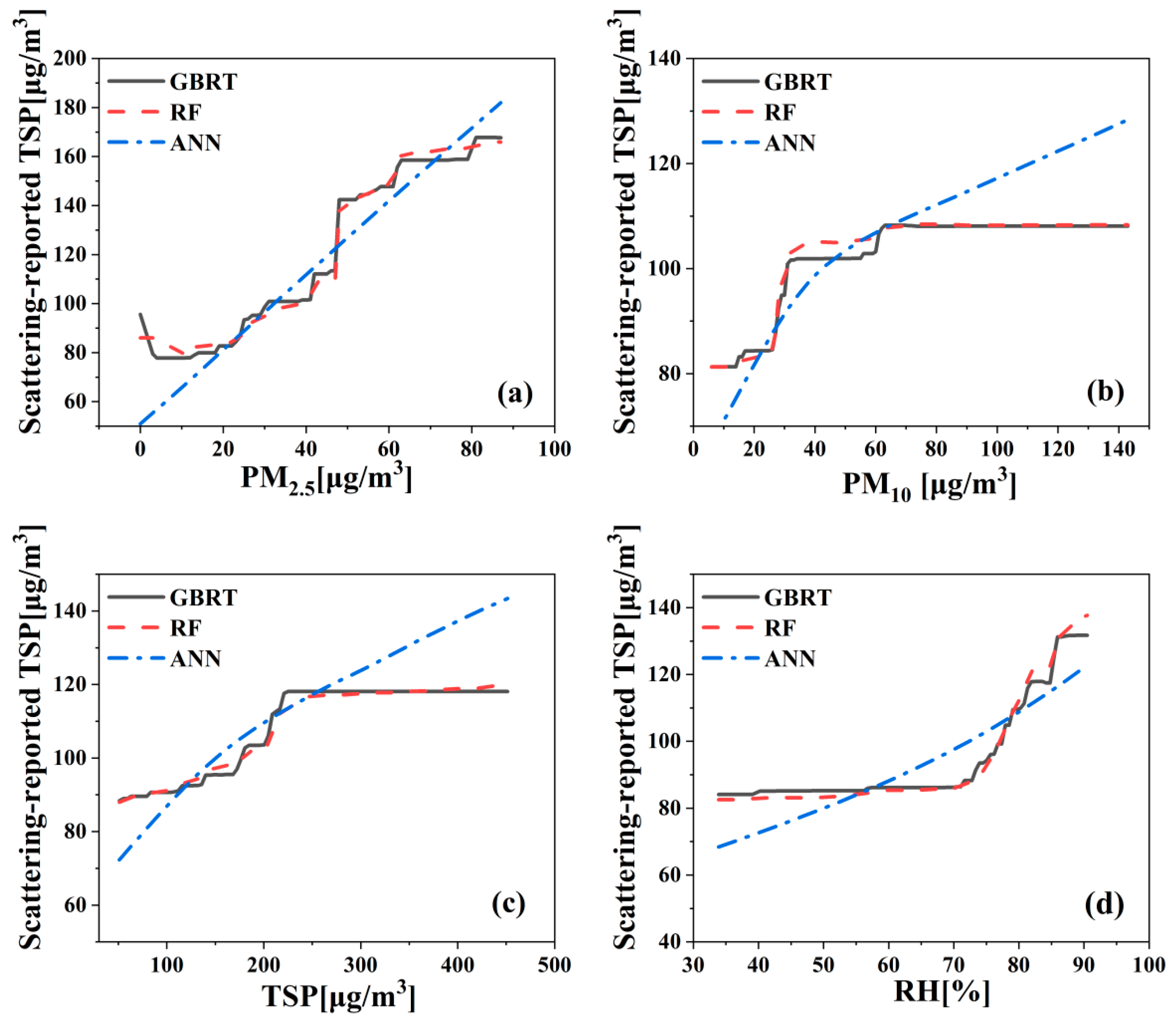
To examine the relative importance of factors, the dependence of the TSP reading from the Casella on one or two factors was examined using one-way or two-way partial dependence plots, respectively. One-way partial dependence of the Casella raw TSP concentrations on the four most significant influencing factors (gravimetric TSP, reference PM2.5, reference PM10, and RH) is plotted and shown in Figure 6. Distinct partial dependence patterns for the four factors were observed. For the factor of PM2.5 concentration (Figure 6a), the Casella-reported TSP concentration increased continuously from 80 to 140 μg/m3 as the PM2.5 mass concentration increased from ~20 to 50 μg/m3; the most rapid increase occurred in the PM2.5 mass range of 22–46 μg/m3. For the factors of PM10 and TSP concentrations (Figure 4b,c), the Casella-reported TSP concentration increased from 85 to ~110 μg/m3 rapidly in the low mass ranges of both PM10 (<60 μg/m3) and TSP (<240 μg/m3) and then leveled off at higher concentrations. Because the Casella derives the TSP concentration from the particle light scattering intensity, the ratio of Casella-reported TSP to the reference PM2.5, PM10, and TSP concentrations can be regarded as an index of aerosol mass scattering efficiency. As a result, the relative aerosol scattering efficiency could be estimated to be 2 for PM2.5, 0.83 for PM10, and 0.2 for TSP. These values are consistent with the theoretical dependence of scattering efficiency on particle size [6]. Light scattering efficiencies are the highest (Mie scattering) for particles with diameters close to the laser wavelength (635 nm for the Casella) and drop off at smaller (Raleigh scattering) and larger sizes (geometric scattering). Particles with diameters near the laser wavelength from a higher mass percentage in PM2.5 than in PM10 and TSP. The influence of RH (Figure 5d) was different from that of the three PM factors. When the RH was less than ~70%, the Casella-reported TSP concentrations were nearly independent of RH; however, when RH was higher than 70%, the Casella-reported TSP concentrations experienced a near-exponential growth, like the classical aerosol hygroscopic growth curve [8,9]. More details of the derived hygroscopic growth factors from PDP will be discussed in Section 3.3.
In terms of performance differences among the three machine learning models, the PDP of the GBRT algorithm was quite close to that of the RF algorithm. The PDP trend of the ANN algorithm was much smoother than those of the other two algorithms. These differences may be caused by the different structures of tree models and neural networks. Each decision tree in a set is independent, and anyone can predict the final response. A neural network is a network connecting neurons. Neurons cannot function without other neurons. Usually, they are grouped by layers and process the data in each layer. The results are passed to the next layer and the neurons in the last layer are responsible for making decisions. In this way, the marginal effect of the tree models is uneven on a small scale because of the difference in individual predictors, while that of the neural network is much smoother because neurons are connected.
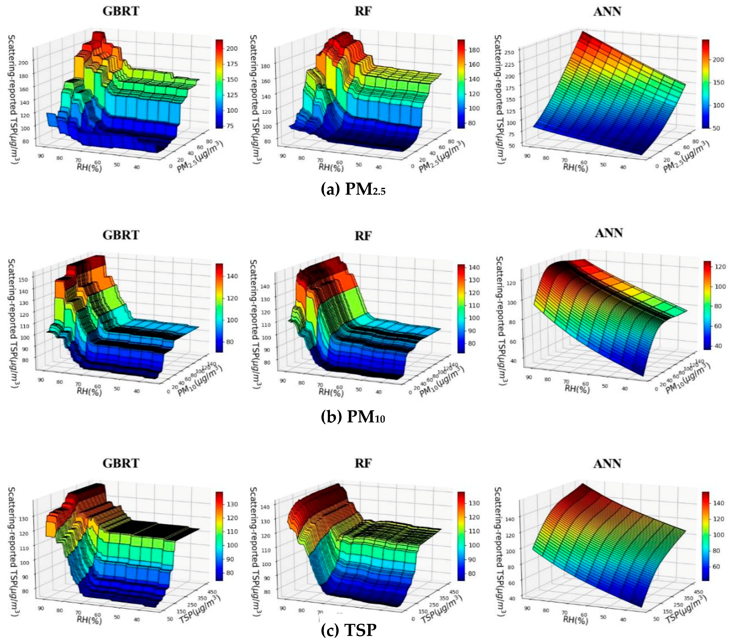
Two-way PDP charts can provide more comprehensive dependence information on the dependence between the target response of light scattering TSP values and PM concentrations (PM2.5, PM10, TSP) as well as RH. Figure 7 shows that for RH lower than 70%, the Casella-reported TSP concentrations were dominantly influenced by PM concentrations, while the influence of RH was negligible. When RH values were higher than 70%, Casella-reported TSP concentrations always experienced near-exponential growth, at all PM concentration levels. Similar to the performance of the one-way PDP charts, the two-way PDP trends of the ANN algorithm were smooth over the entire range, much different from those of the other two algorithms.

3.3. Derivation of Scattering Hygroscopic Growth Curve

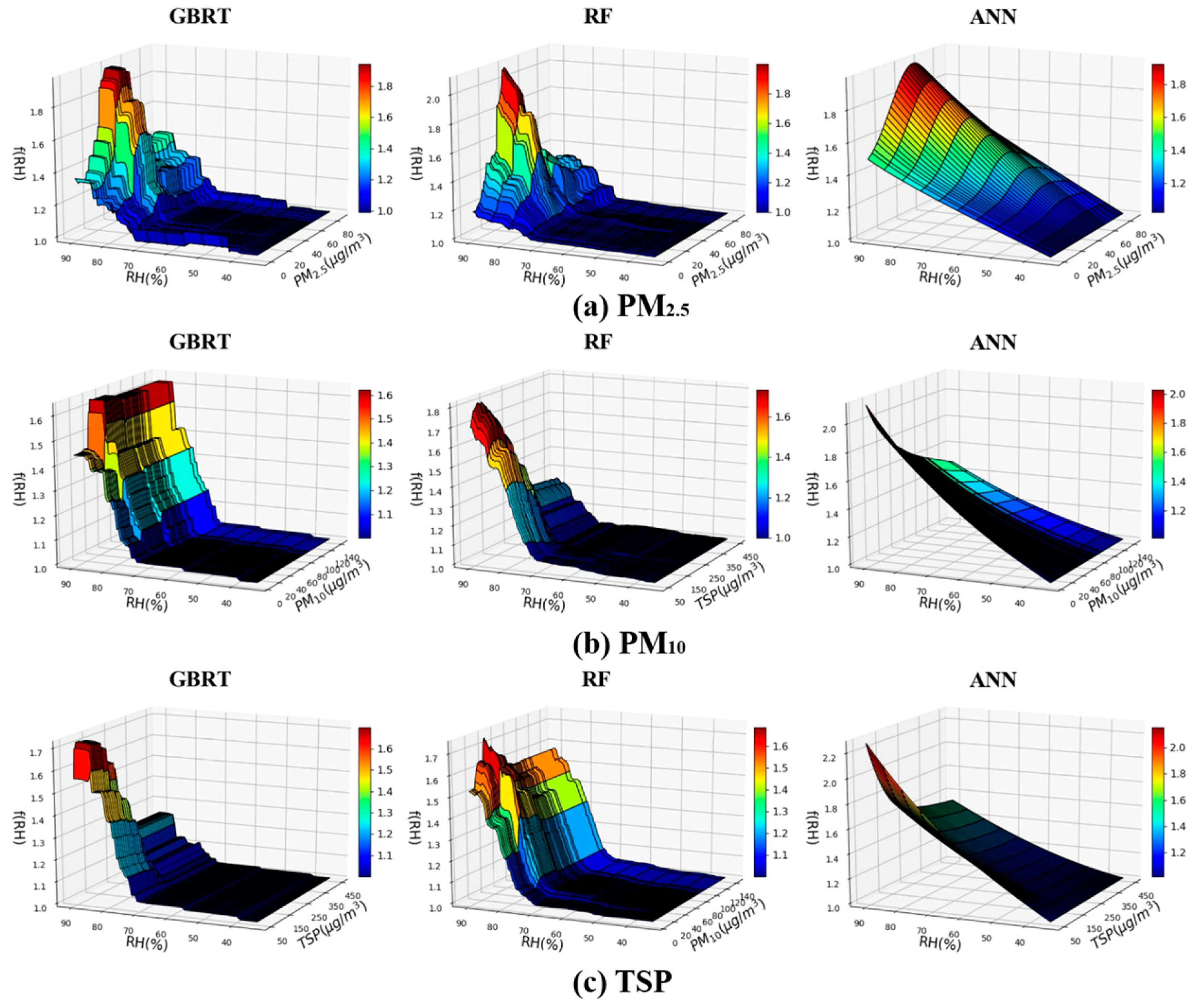
Figure 8 shows the two-way PDP charts between the estimated scattering hygroscopic factor (f(RH)) and PM concentrations (PM2.5, PM10, and TSP) as well as RH for the three machine learning models (i.e., GBRT, RF, and ANN). The hygroscopic curve of RF and GBRT had similar patterns with distinct deliquescence growth at RH ≳ 70%, while that of ANN showed smooth growth without deliquescence growth. The maximum f(RH) values when RH >90% for the ANN were 2.0–2.3, also much higher than the 1.6–2.0 for RF and GBRT. Although both GBRT and RF showed a critical RH of ~70% above which f(RH) showed a significant increase, the trends of f(RH) were different for PM2.5, PM10 and TSP. f(RH) increased with increasing PM2.5 mass concentrations until 40 μg/m3, reached at the maximum value of 1.9–2.1 when RH > 90%, and then decreased with a further increase of the PM2.5 mass concentrations. For PM10, f(RH) increased with increasing PM10 mass concentrations until 50 μg/m3, and then remained at a stable maximum value of 1.6–1.7 when RH > 90%, independent of any further increase in PM10 mass concentration. For TSP, f(RH) reached a maximum of 1.6–1.8 when RH > 90% with a TSP initial mass concentration of 60 μg/m3, then decreased continuously to 1.2 with increasing TSP mass. The different dependence levels of the scattering hygroscopic factor on PM size fractions and concentrations might be related to the different mass fractions of inorganic components such as sulfates and nitrates, which have large hygroscopic growths with distinct growth curves [22]. However, the chemical species percentages in different PM size fractions during the sampling period were not available.
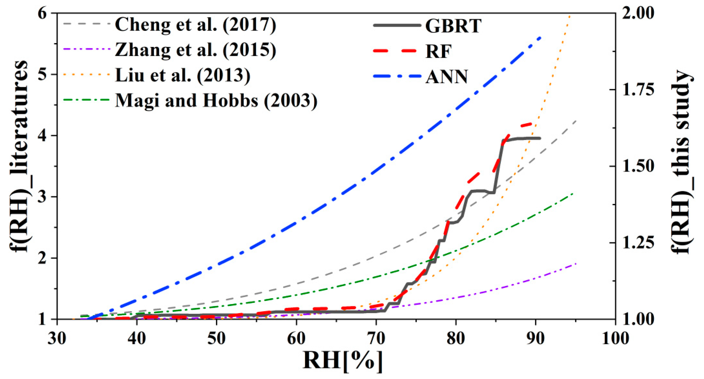
Figure 9 further compares the f(RH) curves from GBRT, RF, and ANN with those from previous studies on ambient aerosol hygroscopic growth. Although most hygroscopic data in the literature refers to the PM2.5 size fraction, the general f(RH) variation patterns are still comparable with those of TSP in this study. In previous studies, Cheng et al. reported an average hygroscopic extinction factor f (RH = 80%) of 2.63 ± 0.45 from 24 cities in China [23]. Zhang et al. found f (RH = 85%) for PM2.5 to be 1.58 ± 0.12 in the Yangtze River Delta of China in March 2013 [24]. Liu et al. estimated that f (RH = 80%) for PM2.5 was 2.01 ± 0.2 at an urban site in the mega-city of Beijing from October 24 to November 9, 2007 [25]. Magi and Hobbs (2003) measured a PM2.5 f (RH = 80%) value of 2.12 ± 0.15 in South Africa, Botswana, Mozambique, and Zambia [26]. In this study, the average f(RH = 80%) values were 1.31, 1.37, and 1.69 derived from GBRT, RF, and ANN, respectively. The f(RH) values of PM2.5 from previous studies are about 1 to 3 times that of TSP in this study, indicating that the scattering hygroscopic efficiency of PM2.5 is much higher than that of TSP. The mass scattering efficiency of PM2.5 is higher than that of PM10 and TSP. This is expected because there are higher proportions of hygroscopic inorganic components in PM2.5 than in TSP. For the specific f(RH) curve versus RH, the pattern from the ANN shows more consistency with the previous PM2.5 pattern than do those from RF and GBRT, although the absolute f(RH) value from the ANN was obviously higher than those from the other two machine learning models.

4. Conclusions

This study explored and applied four machine learning models (SVM, RF, GBRT, ANN) to correct raw TSP concentrations reported by a Casella CEL-712, a light scattering dust monitor. The result shows that all four machine learning models greatly improved the correlation of the TSP concentrations reported by the Casella with filter-based measurements. Partial dependence plots between Casella-reported TSP concentrations and reference PM2.5, PM10, and TSP concentrations and RH provided insights into the main factors influencing the Casella TSP biases. While RH had a negligible influence on TSP concentrations at RH < 70%, near exponential growth in the Casella reported TSP concentrations were observed at RH > 70% by RF and GBRT. When compared with earlier studies on the hygroscopic growth of PM2.5, it was found that the growth factors of TSP were smaller than those of PM2.5, likely due to the lower mass percentage of hygroscopic inorganic species in TSP. Due to the large impact of RH on Casella TSP data accuracy, more data from high RH periods will be collected and used in model training to improve model performance.
Although a significant improvement in Casella TSP accuracy was achieved using machine learning models, there are some limitations that should be addressed in future work: 1) The volume of the dataset was not large enough for deeper machine learning progresses; better model performance is expected with larger a number of hourly data, more monitoring sites, and other parameters that can potentially indicate confounding factors (e.g., traffic volume, wind speed, and direction). 2) TSP concentrations were not measured at the same site as the National monitoring stations, which might cause some discrepancies. Future work should attempt collocated TSP, criteria pollutant, and metrological measurements to obtain matching data. 3) Many of the data in this study were collected at different times at different sites, which made comparison among different sites very difficult. Future work should collect data simultaneously at different sites with better data completeness. 4) This study used 80% of total combined records of all sites to train the models and the remaining 20% records to evaluate model performance due to the huge discrepancy of records amount among stations. The alternative is to use 80% by the number of sites for training and use the remaining 20% sites for model evaluation. A sensitivity study is proposed to estimate the model performance by these two methods in the future. 5) The models were specifically trained for Casella monitors. Future work should evaluate how these models can be extended to other light scattering devices or other types of air quality sensors (e.g., electrochemical CO, SO2, NO2, and O3 sensors).
The emergence of a wide range of low-cost sensors in recent years is changing the paradigm of air quality monitoring, drastically increasing spatial and temporal resolutions. However, corrections of the raw sensor output using machine learning seems indispensable and is a perfect supplement for these sensors. Furthermore, machine learning is no longer a black box with the assistance of interpretability methods. Major factors affecting sensor performance can be probed and diagnosed, and more useful scientific information could be derived from the reconstructed machine learning models.

Author Contributions

Q.G. conducted the model development and validation, data analysis, charts design, and the writing of the manuscript. Z.Z. and S.X. carried out the measurements and collected the raw datasets of TSP. Y.D. provide the measurement data of PM2.5 and PM10 as well as gaseous pollutants. Z.C. and X.W. were responsible for suggestions on the data analysis and revision of the manuscript. All authors have read and agreed to the published version of the manuscript.

Funding

This work was supported by the National Key Research and Development Program of China (2016YFC0208700), National Natural Science Foundation of China (41975152) and the key Research Projects from Shanghai Environmental Protection Bureau (NO. shcg18-10181).

Acknowledgments

We thanks Jun Pan from Shanghai Environmental Monitoring Center for data checking of this study. The authors would like to thank the reviewers and editor for their helpful comments on this manuscript.

Conflicts of Interest

The authors declare no conflict of interest.

References

  1. Chow, J.C. Measurement Methods to Determine Compliance with Ambient Air-Quality Standards for Suspended Particles. Air Waste Manag. Assoc. 1995, 45, 320–382. [Google Scholar] [CrossRef] [PubMed] [Green Version]
  2. Jaklevic, J.M.; Gatti, R.C.; Goulding, F.S.; Loo, B.W. A beta-gage method applied to aerosol samples. Environ. Sci. Technol. 1981, 15, 680–686. [Google Scholar] [CrossRef] [PubMed]
  3. Patashnick, H.; Rupprecht, E.G. Continuous PM-10 measurements using the tapered element oscillating microbalance. Air Waste Manag. Assoc. 1991, 41, 1079–1083. [Google Scholar] [CrossRef]
  4. Black, D.L.; McQuay, M.Q.; Bonin, M.P. Laser-based techniques for particle-size measurement: A review of sizing methods and their industrial applications. Prog. Energy Combust. Sci. 1996, 22, 267–306. [Google Scholar] [CrossRef]
  5. Gebhart, J. Optical direct-reading techniques: Light intensity systems. In Aerosol Measurement: Principles, Techniques, and Applications, 2nd ed.; Baron, P., Willeke, K., Eds.; John Wiley & Sons: New York, NY, USA, 2001; pp. 419–454. [Google Scholar]
  6. Wang, X.L.; Chancellor, G.; Evenstad, J.; Farnsworth, J.E.; Hase, A.; Olson, G.M.; Sreenath, A.; Agarwal, J.K. A Novel Optical Instrument for Estimating Size Segregated Aerosol Mass Concentration in Real Time. Aerosol Sci. Technol. 2009, 43, 939–950. [Google Scholar] [CrossRef]
  7. Covert, D.S.; Charlson, R.J.; Ahlquist, N.C. A study of the relationship of chemical composition and humidity to light scattering by aerosols. J. Appl. Meteorol. 1972, 11, 968–976. [Google Scholar] [CrossRef] [Green Version]
  8. Tang, I.N. Chemical and size effects of hygroscopic aerosols on light scattering coefficients. J. Geophys. Res. 1996, 101, 19245–19250. [Google Scholar] [CrossRef]
  9. Suleiman, A.; Tight, M.R.; Quinn, A.D. Applying machine learning methods in managing urban concentrations of traffic-related particulate matter (PM10 and PM2.5). Atmos. Pollut. Res. 2018, 10, 134–144. [Google Scholar] [CrossRef]
  10. Zou, B.; Wang, M.; Wan, N.; Wilson, J.G.; Fang, X.; Tang, Y. Spatial modeling of PM2.5 concentrations with a multifactoral radial basis function neural network. Environ. Sci. Pollut. Res. 2015, 22, 10395–10404. [Google Scholar] [CrossRef]
  11. Sayegh, A.; Tate, J.E.; Ropkins, K. Understanding how roadside concentrations of NOx are influenced by the background levels, traffic density, and meteorological conditions using Boosted Regression Trees. Atmos. Environ. 2016, 127, 163–175. [Google Scholar] [CrossRef]
  12. CEL-712 Dust Detective Kit. Available online: https://www.casellasolutions.com/products/casella_default/cel-712-dust-detective-kit.html (accessed on 11 November 2019).
  13. Szymanski, W.W.; Nagy, A.; Czitrovszky, A.R. Optical particle spectrometry—Problems and prospects. J. Quant. Spectrosc. Radiat. Transfer. 2009, 110, 918–929. [Google Scholar] [CrossRef]
  14. Chunming, W.; Xinbiao, L.; Xiaofeng, C.; Yalong, M.; Chen, C. Application of support vector regression to predict metallogenic favourability degree. Int. J. Phys. Sci. 2010, 5, 5. [Google Scholar]
  15. Cherkassky, V.; Ma, Y. Practical selection of SVM parameters and noise estimation for SVM regression. Neural Netw. 2004, 17, 113–126. [Google Scholar] [CrossRef] [Green Version]
  16. Hu, X.; Belle, J.H.; Meng, X.; Wildni, A.; Waller, L.A.; Strickland, M.J.; Liu, Y. Estimating PM2.5 Concentrations in the Conterminous United States Using the Random Forest Approach. Environ. Sci. Technol. 2017, 51, 6936–6944. [Google Scholar] [CrossRef] [PubMed]
  17. Xiao, Q.; Chang, H.H.; Geng, G.; Liu, Y. An Ensemble Machine-Learning Model To Predict Historical PM2.5 Concentrations in China from Satellite Data. Environ. Sci. Technol. 2018, 52, 13260–13269. [Google Scholar] [CrossRef] [PubMed]
  18. Brokamp, C.; Jandarov, R.; Hossain, M.; Ryan, P. Predicting Daily Urban Fine Particulate Matter Concentrations Using a Random Forest Model. Environ. Sci. Technol. 2018, 52, 4173–4179. [Google Scholar] [CrossRef]
  19. Elith, J.; Leathwick, J.R.; Hastie, T. A working guide to boosted regression trees. J. Animal Ecol. 2008, 77, 802–813. [Google Scholar] [CrossRef]
  20. Zimmerman, N.; Presto, A.A.; Kumar, S.P.N.; Gu, J.; Hauryliuk, A.; Robinson, E.S.; Robinson, A.L.; Subramanian, R. A machine learning calibration model using random forests to improve sensor performance for lower-cost air quality monitoring. Atmos. Meas. Tech. 2018, 11, 291–313. [Google Scholar] [CrossRef] [Green Version]
  21. Friedman, J.H. Greedy Function Approximation: A Gradient Boosting Machine. Ann. Stat. 2001, 29, 1189–1232. [Google Scholar] [CrossRef]
  22. Martin, S.T. Phase Transitions of Aqueous Atmospheric Particles. Chem. Rev. 2000, 100, 3403–3454. [Google Scholar] [CrossRef]
  23. Cheng, Z.; Ma, X.; He, Y.; Jiang, J.; Wang, X.; Wang, Y.; Sheng, L.; Hu, J.; Yan, N. Mass extinction efficiency and extinction hygroscopicity of ambient PM2.5 in urban China. Environ. Res. 2017, 156, 239–246. [Google Scholar] [CrossRef] [PubMed]
  24. Zhang, L.; Sun, J.Y.; Shen, X.J.; Zhang, Y.M.; Che, H.; Ma, Q.L.; Ogren, J.A. Observations of relative humidity effects on aerosol light scattering in the Yangtze River Delta of China. Atmos. Chem. Phys. 2015, 15, 8439–8454. [Google Scholar] [CrossRef] [Green Version]
  25. Liu, X.; Gu, J.; Li, Y.; Cheng, Y.; Qu, Y.; Han, T.; Zhang, Y. Increase of aerosol scattering by hygroscopic growth: observation, modeling, and implications on visibility. Atmos. Res. 2013, 132, 91–101. [Google Scholar] [CrossRef]
  26. Magi, B.I.; Hobbs, P.V. Effects of humidity on aerosols in southern Africa during the biomass burning season. J. Geophys. Res. Atmos. 2003, 108. [Google Scholar] [CrossRef]
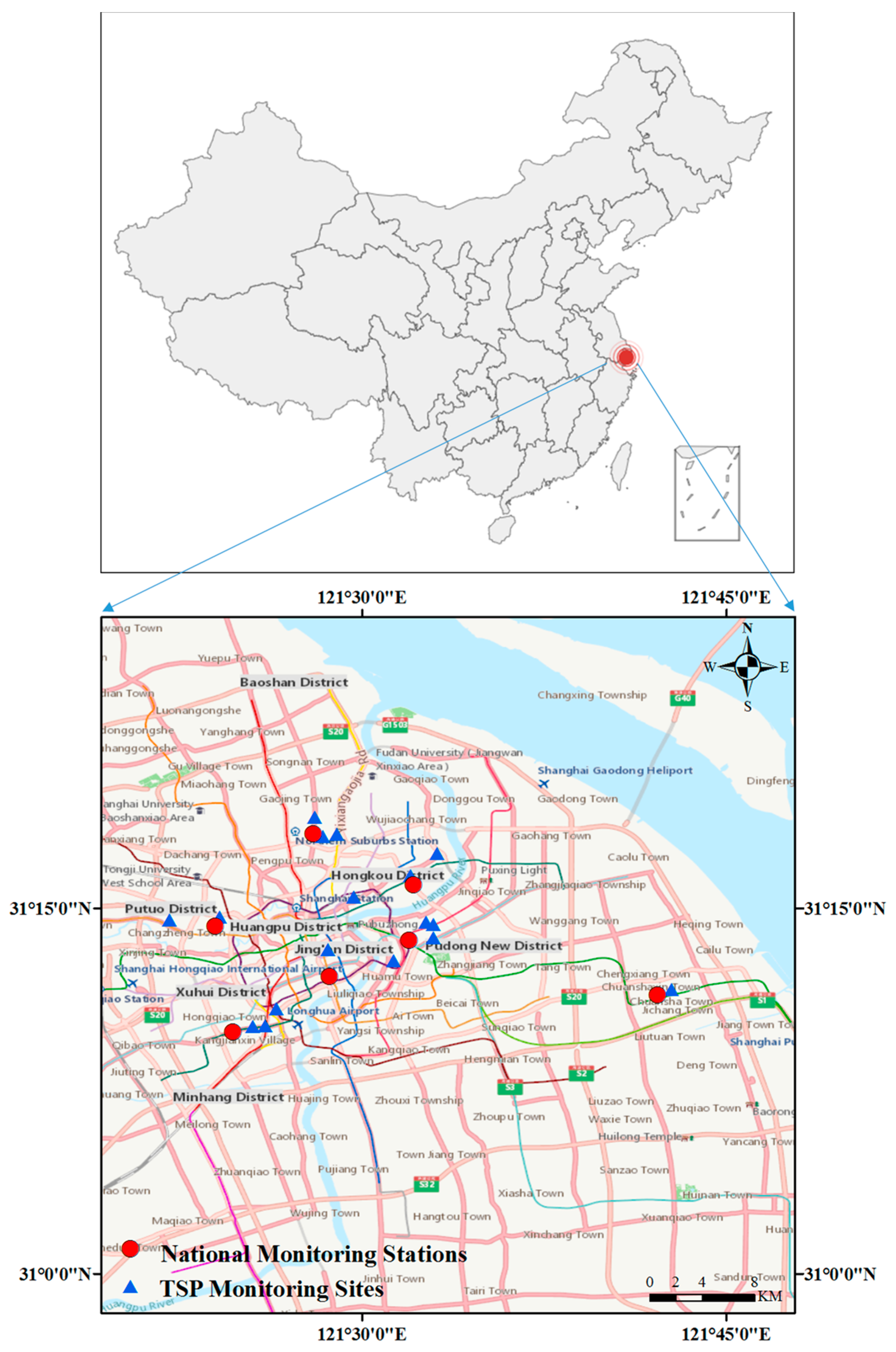
Figure 1. Geographical locations of 17 total suspended particulate (TSP) monitoring sites and 7 national monitoring stations in the urban area of the megacity of Shanghai, China. The blue triangle symbols () represent TSP monitoring sites, which include measurements of TSP concentrations by light scattering and gravimetry, as well as ambient temperature and relative humidity. The red circle symbols () represent national monitoring stations which include the measurements of mass concentrations of PM2.5, PM10, SO2, NO2, CO, and O3.
Atmosphere 11 00139 g001
Figure 2. Comparison of TSP concentrations determined by light scattering and machine learning model outputs with those by gravimetric analyses. (a) LR: Linear Regression; (b) SVM: Support Vector Machine; (c) RF: Random Forest; (d) GBRT: Gradient Boosting Regression Tree; (e) ANN: Artificial Neural Network. y/x represents the slope, R2 is the coefficient of determination, N means the volume of the dataset.
Atmosphere 11 00139 g002
Figure 3. Time series of TSP concentrations obtained from gravimetric measurement, raw Casella reading, and Casella readings corrected by four machine learning models (SVM, RF, GBRT, and ANN). The illustrated data were obtained from the CaoXi Road site over three periods: 15 June 2017 to 22 June 2017, 23 February 2018 to 27 February 2018 and 15 June 2018 to 30 June 2018.
Atmosphere 11 00139 g003
Figure 4. Feature importance analysis on ten factors including PM concentrations (PM2.5, PM10, and TSP), gaseous pollutant concentrations (CO, O3, SO2, and NO2), temperature, relative humidity, and the morning hour of the day. (a) Random forest features importance, (b) SVM ablation study, (c) GBRT ablation study, (d) ANN ablation study.
Atmosphere 11 00139 g004
Figure 5. The correlation coefficient between all the input features. The black blocks represent the coefficients higher than 0.3 while the red blocks represent coefficients lower than −0.3. The white blocks represent the coefficients between −0.3 and 0.3.
Atmosphere 11 00139 g005
Figure 6. Partial dependence of Casella raw TSP concentrations on four influencing factors: (a) PM2.5 concentration, (b) PM10 concentration, (c) gravimetric TSP concentration, (d) relative humidity.
Atmosphere 11 00139 g006
Figure 7. Two-way partial dependence plot of Casella-reported TSP concentration on relative humidity and particulate matter concentration. (a), (b), and (c) represents different particle size of PM2.5, PM10, and TSP, respectively.
Atmosphere 11 00139 g007
Figure 8. Partial dependence plot of estimated hygroscopic growth factor dependence on relative humidity and particulate matter concentration. (a), (b), and (c) represent different particle sizes of PM2.5, PM10, and TSP, respectively.
Atmosphere 11 00139 g008
Figure 9. Comparison of scattering hygroscopic growth curves from three machine learning models (GBRT, RF, and ANN) with previous studies. The hygroscopic growth factor f(RH) of this study (marked with the secondary Y-axis) refers to TSP and is estimated by the Casella -reported TSP concentrations at any ambient RH divided by the scattering TSP concentration value when ambient RH was 40%. Previous studies of hygroscopic growth factor refer to PM2.5 and were marked with the primary Y-axis.
Atmosphere 11 00139 g009
Table 1. Information about all the total suspended particulate (TSP) monitoring sites and their nearby national monitoring stations.
No.TSP Monitoring Sites aNearby National Monitoring Stations bData VolumeDistance (km)Comments
1CX S.-5583.3The same site
2CX R.SSD1063.5Validation site
3GSY&XQ R.SSD402.2
4GL&GSY R.SSD401.4
5JD&DX R.PD201.6
6PDN&WS R.PD301.9
7YS R.PD301.9
8ZY&TL R.PD301.7
9CZ&YQ R.HK301.2
10CZN&SD R.HK301.5
11GY&WSD R.HK200.63
12ZJZ&NJ R.YP302.8
13LZ&CY R.YP300.69
14DDH&MC R.PT300.7
15JY&ZL R.PT303
16FXZ&CQN R.SWC301.8
17CHN&CH R.CS300.97
a: TSP sites cover the measurement indices of ambient TSP online and offline mass, ambient relative humidity and temperature. b: National Monitoring stations cover the measurement indices of ambient PM10, PM2.5, CO, SO2, NO2, and O3.
Table 2. Predictors used to model TSP concentrations and their corresponding measurement instruments.
PredictorsUnitMeasurement Instruments
Scattering TSP concentrationsμg/m3CEL-712, Casella
Hourly PM10 concentrationsμg/m3TEOM1405, Thermo Fisher Scientific
Hourly PM2.5 concentrationsμg/m3TEOM1405FDMS, Thermo Fisher
Hourly SO2 concentrationsμg/m343iSO2 analyzer, Thermo Fisher
Hourly NO2 concentrationsμg/m342iNOX analyzer, Thermo Fisher
Hourly CO concentrationsμg/m348iCO analyzer, Thermo Fisher
Hourly O3 concentrationsμg/m349i O3 analyzer, Thermo Fisher
Hourly ambient temperaturedegree Celsius (°C)Hengxin AZ-8809 Temp./RH Recorder
Hourly ambient relative humiditypercent (%)Hengxin AZ-8809 Temp./RH Recorder
Table 3. Testing performance of the machine learning (ML) models.
ML ModelsSlopeR2MSE (µg/m3)2 RMSE (µg/m3)MAE (µg/m3)
Original Measurement0.410.10---
SVM0.910.762401.5249.0124.19
RF1.020.822453.5249.5324.71
GBRT1.000.782861.0753.4930.15
ANN1.110.902723.4252.1929.18
Table 4. Comparison of machine learning model performances at the CaoXi Road site.
Time PeriodGravimetric Results (μg/m3)Casella Results (μg/m3)SVM (μg/m3)RF (μg/m3)GBRT (μg/m3)ANN (μg/m3)
15 June 2017 to 22 June 2017132.2292.28132.85 133.15132.53134.04
23 February 2018 to 27 February 2018121.15108.10114.96 119.92120.71119.83
15 June 2018 to 30 June 2018107.7394.53104.82107.94107.73107.96