The Effect of Boreal Summer Intraseasonal Oscillation on Evaporation Duct and Electromagnetic Propagation over the South China Sea


Abstract
1. Introduction
2. Data and Methods
2.1. Data
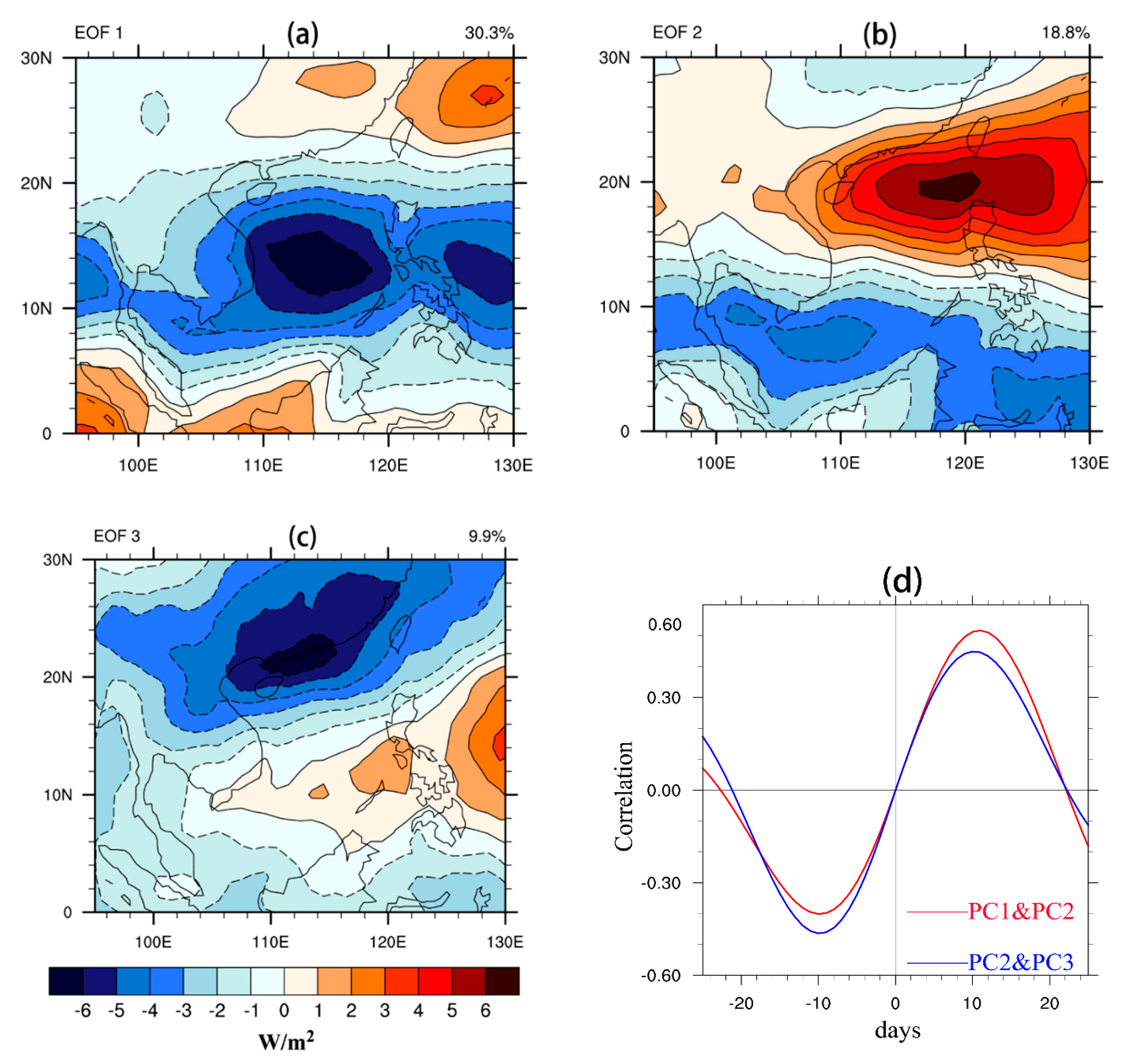
2.2. BSISO Analysis
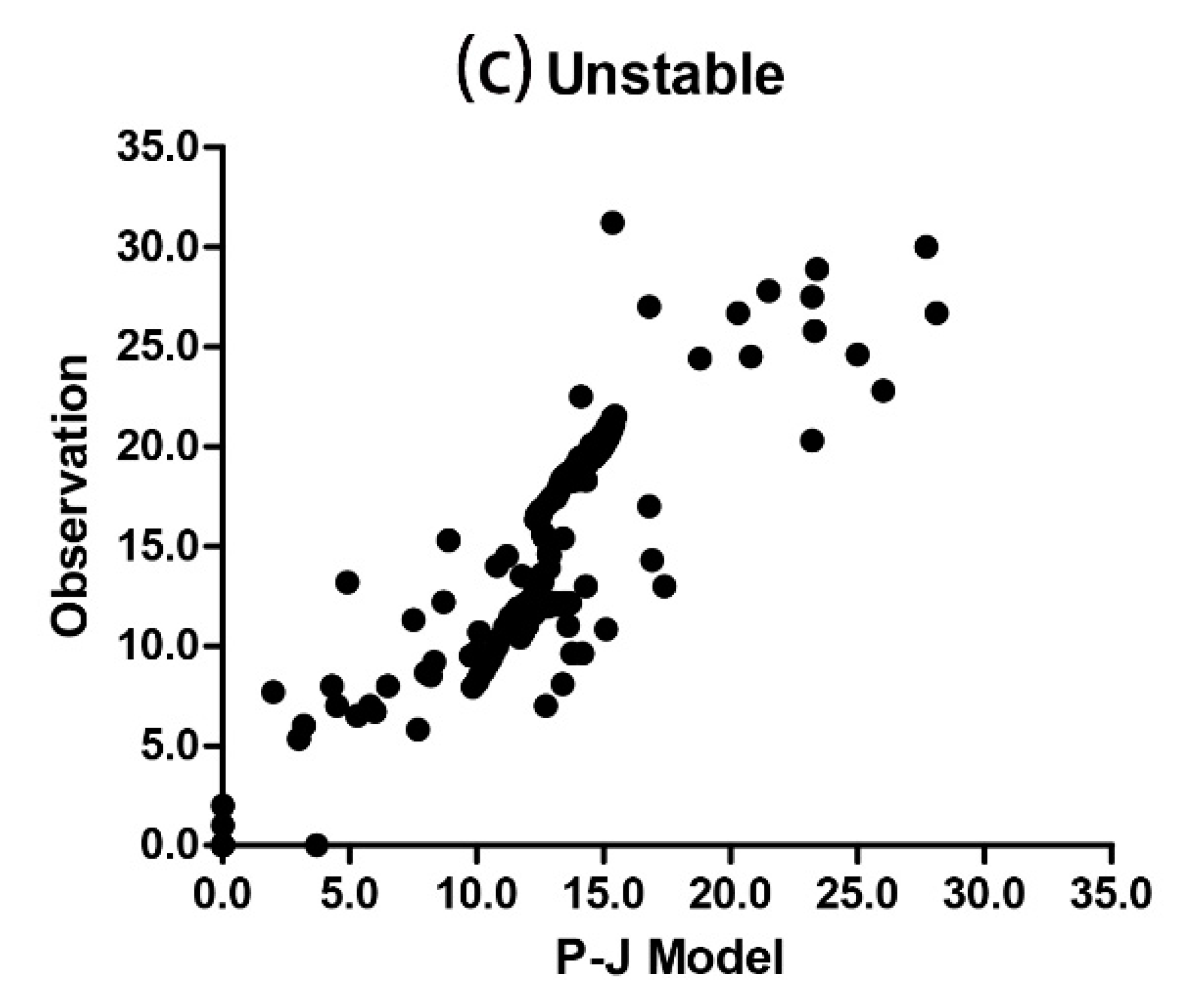
2.3. Paulus-Jeske (P-J) Model
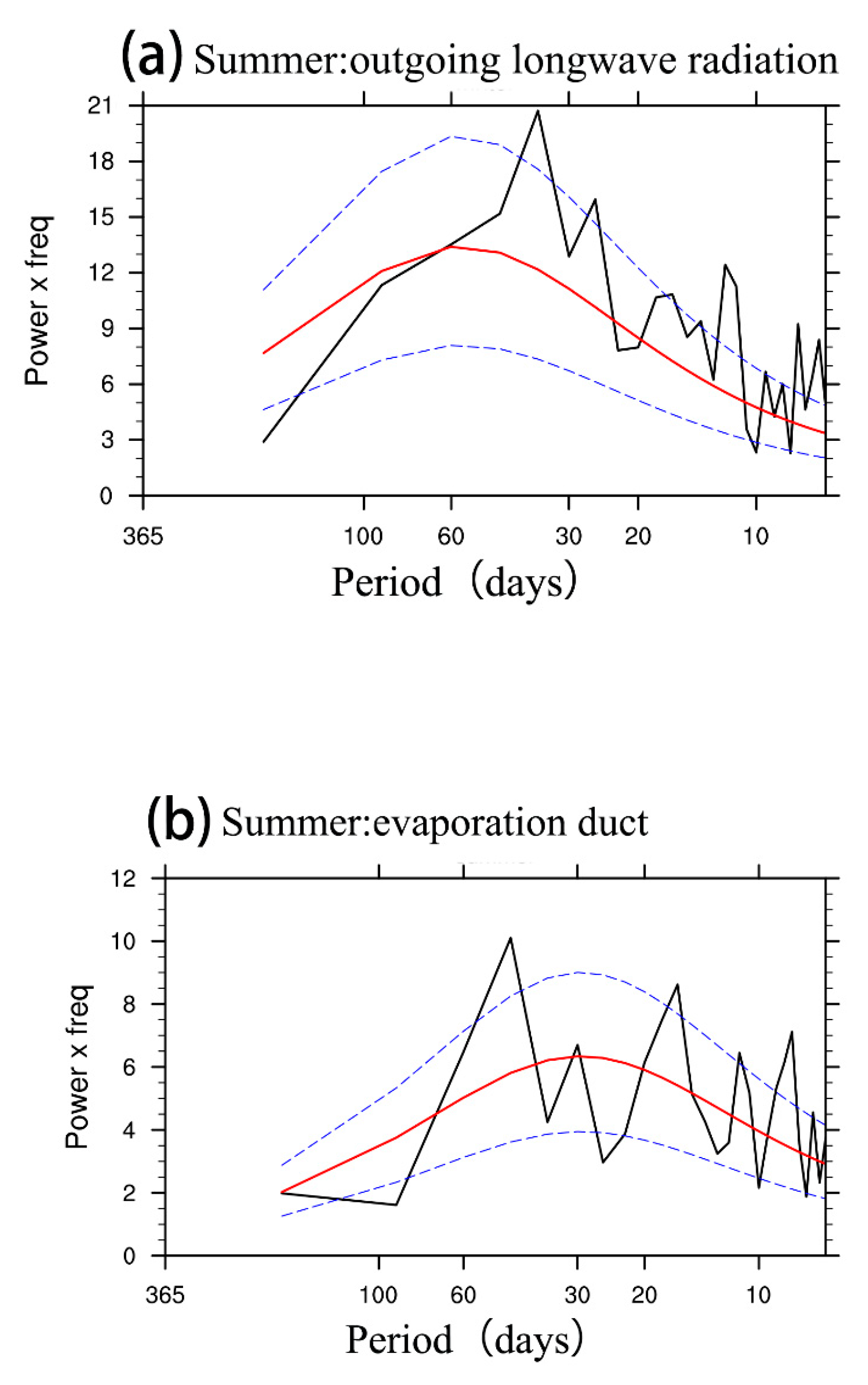
3. ISO of Evaporation Duct
4. ISO of Evaporation Duct
4.1. Correlation Analysis
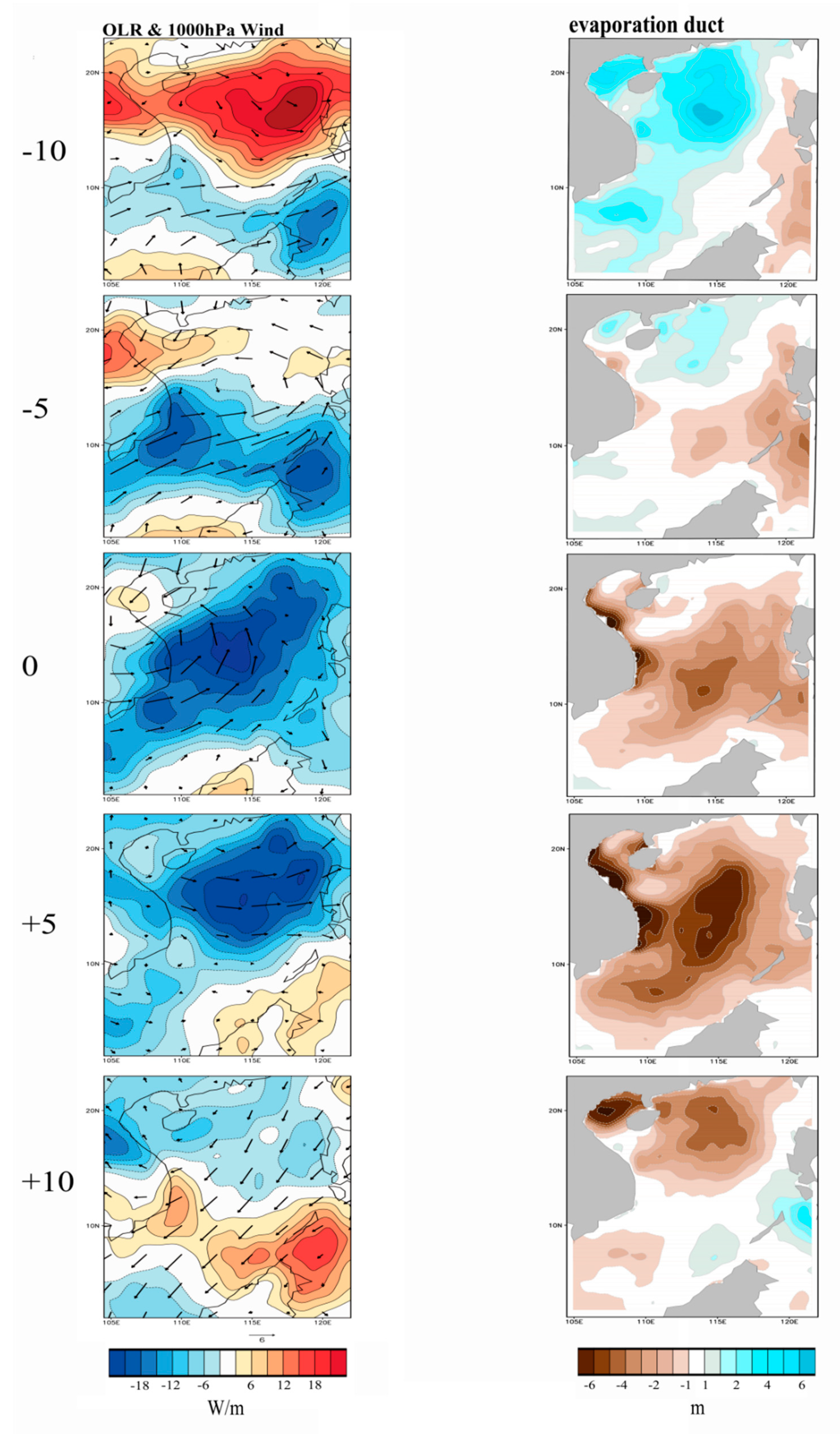
4.2. Composite Analysis
5. The Effect of BSISO on Evaporation Duct
5.1. Meteorological Factors Influencing the Evaporation Duct
5.2. Schematic Analysis
6. The Effect of Evaporation Duct on Electromagnetic Propagation
6.1. Parabolic Equation
6.2. Electromagnetic Simulation
7. Conclusions
- The P-J model is suitable for characterizing the evaporation duct over the SCS area in summer. As a result of the BSISO, the evaporation duct exhibits an intraseasonal oscillation of 30–60 days, and shows strong correlation between certain time-space distribution features. The height and strength of the evaporation duct is enhanced/suppressed in negative/positive phases of the BSISO, leading to the development of a negative/positive center in evaporation duct anomalies to the south of the active/inactive BSISO convection. These two features do not exactly co-occur, and the evolution of evaporation duct lags behind the BSISO-related convection by about 2–4 days.
- Changes in the difference of temperature and humidity at the air–sea layer caused by BSISO-related convection are the dominant factors influencing the evaporation duct. Clouds, precipitation, and enhanced southwest airflow can reduce differences in air–sea temperature and humidity throughout the area of active convection, thus weakening the strength and height of the evaporation duct. Conversely, the duct will be significantly enhanced on sunny days.
- Based on observational data from a meteorological station in the SCS, we calculated the evaporation duct and modified refractivity profiles in typical negative and positive phases of the BSISO. The propagation of electromagnetic waves during conditions of different evaporation ducts was also simulated by the PE model. During the negative phase of BSISO convection, a strong evaporation duct causes significant over-the-horizon propagation and the development of blind areas, causing the electromagnetic fields to differ obviously from standard atmospheric conditions.
Author Contributions
Funding
Acknowledgments
Conflicts of Interest
References
- Bean, B.R.; Dutton, E.J. Radio Meteorology; Dover Publication Inc.: New York, NY, USA, 1968; p. 435. [Google Scholar]
- Cook, J. A sensitivity study of weather data inaccuracies on evaporation duct height algorithms. Radio Sci. 1991, 26, 731–746. [Google Scholar] [CrossRef]
- Jeske, H. State and Limits of Prediction Methods of Radar Wave Propagation Conditions Over Sea; Springer: Dordrecht, The Netherlands, 1973. [Google Scholar]
- Paulus, R.A. Practical application of an evaporation duct model. Radio Sci. 1985, 20, 887–896. [Google Scholar] [CrossRef]
- Musson-Genon, L.; Gauthier, S.; Bruth, E. A simple method to determine evaporation duct height in the sea surface boundary layer. Radio Sci. 1992, 27, 635–644. [Google Scholar] [CrossRef]
- Babin, S.M. A New Model of the Oceanic Evaporation Duct and Its Comparison with Current Models. Ph.D. Thesis, University of Maryland, College Park, MD, USA, 1996. [Google Scholar]
- Zhu, X.; Li, J.; Zhu, M.; Jiang, Z.; Li, Y. An Evaporation Duct Height Prediction Method Based on Deep Learning. IEEE Geosci. Remote Sens. Lett. 2018, 15, 1307–1311. [Google Scholar] [CrossRef]
- Dockery, G. Modeling electromagnetic wave propagation in the troposphere using the parabolic equation. IEEE Trans. Antennas Propag. 1988, 36, 1464–1470. [Google Scholar] [CrossRef]
- Ding, J.L.; Fei, J.F.; Huang, X.G.; Zhang, X.; Zhou, X.; Tian, B. Contrast on occurrence of evaporation ducts in the South China Sea and East China Sea area. Chin. J. Radio Sci. 2009, 24, 1018–1023. (In Chinses) [Google Scholar]
- Wang, B.; Xie, X. A Model for the Boreal Summer Intraseasonal Oscillation. J. Atmos. Sci. 1997, 54, 72–86. [Google Scholar] [CrossRef]
- Wang, B.; Webster, P.J.; Kikuchi, K.; Yasunari, T.; Qi, Y. Boreal summer quasi-monthly oscillation in the global tropics. Clim. Dyn. 2006, 27, 661–675. [Google Scholar] [CrossRef]
- Lee, J.-Y.; Wang, B.; Wheeler, M.C.; Fu, X.; Waliser, D.E.; Kang, I.-S. Real-time multivariate indices for the boreal summer intraseasonal oscillation over the Asian summer monsoon region. Clim. Dyn. 2013, 40, 493–509. [Google Scholar] [CrossRef]
- Lawrence, D.M.; Webster, P.J. The Boreal Summer Intraseasonal Oscillation: Relationship between Northward and Eastward Movement of Convection. J. Atmos. Sci. 2002, 59, 1593–1606. [Google Scholar] [CrossRef]
- Yasunari, T. Cloudiness Fluctuations Associated with the Northern Hemisphere Summer Monsoon. J. Meteorol. Soc. Jpn. 1979, 57, 227–242. [Google Scholar] [CrossRef]
- Kemball-Cook, S.; Wang, B. Equatorial Waves and Air–Sea Interaction in the Boreal Summer Intraseasonal Oscillation. J. Clim. 2001, 14, 2923–2942. [Google Scholar] [CrossRef]
- Annamalai, H.; Sperber, K.R. Regional Heat Sources and the Active and Break Phases of Boreal Summer Intraseasonal (30–50 Day) Variability. J. Atmos. Sci. 2005, 62, 2726–2748. [Google Scholar] [CrossRef]
- Sengupta, D.; Ravichandran, M. Oscillations of Bay of Bengal sea surface temperature during the 1998 Summer Monsoon. Geophys. Res. Lett. 2001, 28, 2033–2036. [Google Scholar] [CrossRef]
- Hendon, H.H.; Glick, J. Intraseasonal Air–Sea Interaction in the Tropical Indian and Pacific Oceans. J. Clim. 1997, 10, 647–661. [Google Scholar] [CrossRef]
- Klingaman, N.P.; Weller, H.; Slingo, J.M.; Inness, P.M. The Intraseasonal Variability of the Indian Summer Monsoon Using TMI Sea Surface Temperatures and ECMWF Reanalysis. J. Clim. 2008, 21, 2519–2539. [Google Scholar] [CrossRef]
- Wang, T.; Yang, X.-Q.; Fang, J.; Sun, X.; Ren, X. Role of Air–Sea Interaction in the 30–60-Day Boreal Summer Intraseasonal Oscillation over the Western North Pacific. J. Clim. 2018, 31, 1653–1680. [Google Scholar] [CrossRef]
- Dee, D.P.; Uppala, S.M.; Simmons, A.J.; Berrisford, P.; Poli, P.; Kobayashi, S.; Andrae, U.; Balmaseda, M.A.; Balsamo, G.; Bauer, D.P.; et al. The ERA-Interim reanalysis: Configuration and performance of the data assimilation system. Q. J. R. Meteorol. Soc. 2011, 137, 553–597. [Google Scholar] [CrossRef]
- Liebmann, B. Description of a complete (interpolated) outgoing longwave radiation dataset. Bull. Am. Meteorol. Soc. 1996, 77, 1275–1277. [Google Scholar]
- Yu, L.; Jin, X.; Weller, R.A. Multidecade Global Flux Datasets from the Objectively Analyzed Air-Sea Fluxes (OAFlux) Project: Latent and Sensible Heat Fluxes, Ocean Evaporation, and Related Surface Meteorological Variables; OAFlux Project Technical Report (OA-2008-01); Woods Hole Oceanographic Institution: Woods Hole, MA, USA, 2008; 64p. [Google Scholar]
- Kummerow, C.; Simpson, J.; Thiele, O.; Barnes, W.; Chang, A.T.; Stocker, E.; Adler, R.F.; Hou, A.; Kakar, R.; Wentz, F.; et al. The Status of the Tropical Rainfall Measuring Mission (TRMM) after Two Years in Orbit. J. Appl. Meteorol. 2000, 39, 1965–1982. [Google Scholar] [CrossRef]
- Duchon, C.E. Lanczos filtering in one and two dimensions. J. Appl. Meteorol. 1979, 18, 1016–1022. [Google Scholar] [CrossRef]
- Yao, J.X.; Li, L.P.; Luo, X.; Yang, W.; Wang, P.X. Lanczos filter suitable for filtering quasi-two-week and quasi-one-month oscillations and its applications. Trans. Atmos. Sci. 2012, 2, 221–228. [Google Scholar]
- Liu, W.T.; Katsaros, K.B.; Businger, J.A. Bulk Parameterization of Air-Sea Exchanges of Heat and Water Vapor Including the Molecular Constraints at the Interface. J. Atmos. Sci. 1979, 36, 1722–1735. [Google Scholar] [CrossRef]
- Paulus, R.A. Specification for Evaporation Duct Height Calculations; Naval Ocean Systems Center: San Diego, CA, USA, 1989. [Google Scholar]
- Xie, S.; Philander, S.G. A coupled ocean-atmosphere model of relevance to the ITCZ in the eastern Pacific. Tellus A 1994, 46, 340–350. [Google Scholar] [CrossRef]
- Mahajan, S.; Saravanan, R.; Chang, P. The Role of the Wind–Evaporation–Sea Surface Temperature (WES) Feedback as a Thermodynamic Pathway for the Equatorward Propagation of High-Latitude Sea Ice–Induced Cold Anomalies. J. Clim. 2011, 24, 1350–1361. [Google Scholar] [CrossRef]
- Zeng, L.L.; Shi, P.; Wang, D.X.; Chen, J. Seasonal and interannual variabilities of evaporation and net freshwater flux in the South China Sea. Chin. J. Geophys. 2009, 52, 929–938. [Google Scholar]
- Fairall, C.W.; Bradley, E.F.; Rogers, D.P.; Edson, J.B.; Young, G.S. Bulk parameterization of air-sea fluxes for Tropical Ocean-Global Atmosphere Coupled-Ocean Atmosphere Response Experiment. J. Geophys. Res. Space Phys. 1996, 101, 3747–3764. [Google Scholar] [CrossRef]
- Fairall, C.W.; Bradley, E.F.; Hare, J.E.; Grachev, A.A.; Edson, J.B. Bulk Parameterization of Air-Sea Fluxes: Updates and Verification for the COARE Algorithm. J. Clim. 2003, 16, 571–591. [Google Scholar] [CrossRef]
- Kuttler, J.R.; Dockery, G.D. Theoretical description of the parabolic approximation/Fourier split-step method of representing electromagnetic propagation in the troposphere. Radio Sci. 1991, 26, 381–393. [Google Scholar] [CrossRef]
- Akbarpour, R.; Webster, A. Ray-tracing and parabolic equation methods in the modeling of a tropospheric microwave link. IEEE Trans. Antennas Propag. 2005, 53, 3785–3791. [Google Scholar] [CrossRef]
- Barrios, A.E. A terrain parabolic equation model for propagation in the troposphere. IEEE Trans. Antennas Propag. 1994, 42, 90–98. [Google Scholar] [CrossRef]


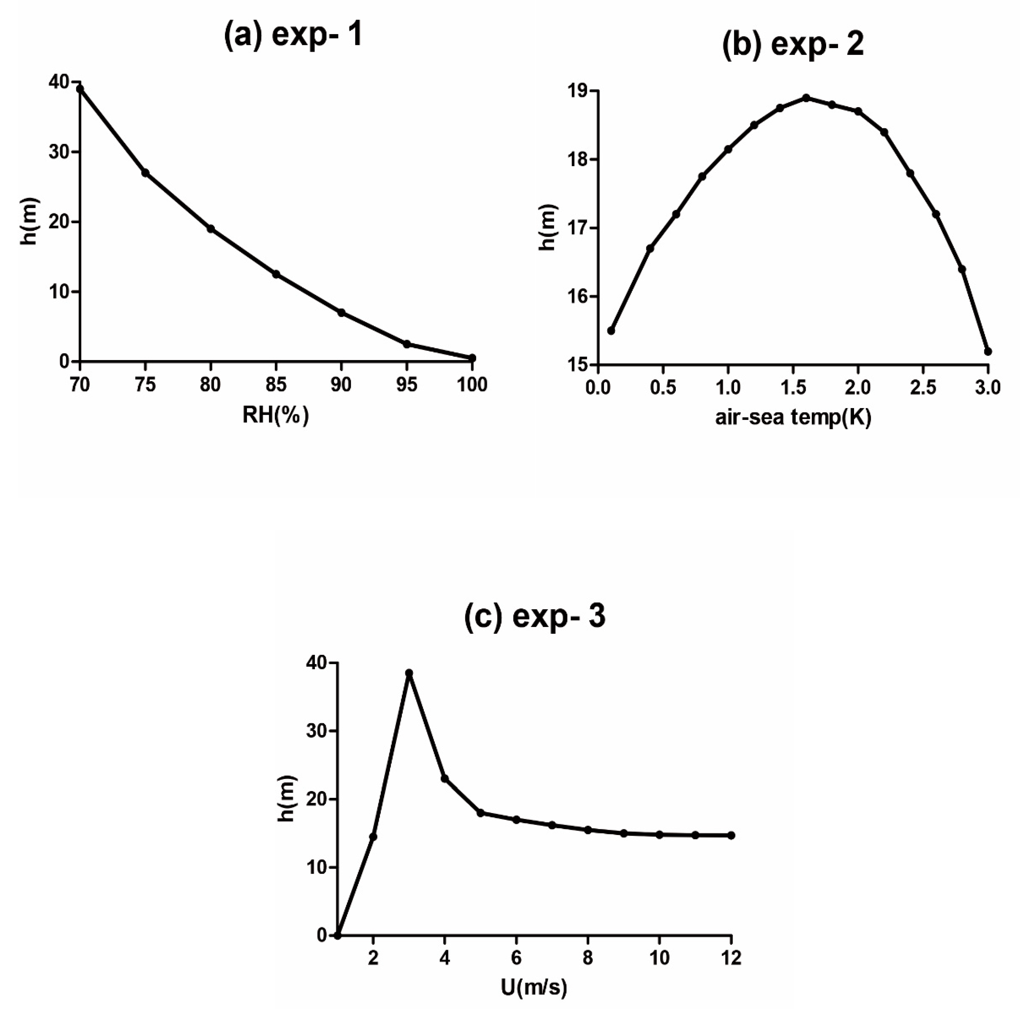
| Wind | Humidity | Air Temperature | Sea Surface Temperature | Pressure | |
|---|---|---|---|---|---|
| exp-1 | 5 m/s | 100%~70% | 25.5 °C | 25 °C | 1015 hPa |
| exp-2 | 5 m/s | 80% | 25~28 °C | 25 °C | 1015 hPa |
| exp-3 | 1~12 m/s | 80% | 25.5 °C | 25 °C | 1015 hPa |
| Frequency | Antenna | Vertical Beam Width | Elevation | Aerial Gain |
| 6 GHz | gauss | 3° | 0° | 29 dB |
| Polarization Mode | Antenna Height | Receiver Sensitivity | Peak Power | RCS |
| HH | 20 m | −110 dBm | 300 kW | 100 m2 |
Publisher’s Note: MDPI stays neutral with regard to jurisdictional claims in published maps and institutional affiliations. |
© 2020 by the authors. Licensee MDPI, Basel, Switzerland. This article is an open access article distributed under the terms and conditions of the Creative Commons Attribution (CC BY) license (http://creativecommons.org/licenses/by/4.0/).
Share and Cite
Jia, W.; Zhang, W.; Zhu, J.; Sun, J. The Effect of Boreal Summer Intraseasonal Oscillation on Evaporation Duct and Electromagnetic Propagation over the South China Sea. Atmosphere 2020, 11, 1298. https://doi.org/10.3390/atmos11121298
Jia W, Zhang W, Zhu J, Sun J. The Effect of Boreal Summer Intraseasonal Oscillation on Evaporation Duct and Electromagnetic Propagation over the South China Sea. Atmosphere. 2020; 11(12):1298. https://doi.org/10.3390/atmos11121298
Chicago/Turabian StyleJia, Wentao, Weimin Zhang, Jiahua Zhu, and Jilin Sun. 2020. "The Effect of Boreal Summer Intraseasonal Oscillation on Evaporation Duct and Electromagnetic Propagation over the South China Sea" Atmosphere 11, no. 12: 1298. https://doi.org/10.3390/atmos11121298
APA StyleJia, W., Zhang, W., Zhu, J., & Sun, J. (2020). The Effect of Boreal Summer Intraseasonal Oscillation on Evaporation Duct and Electromagnetic Propagation over the South China Sea. Atmosphere, 11(12), 1298. https://doi.org/10.3390/atmos11121298