Abstract
Over time, the initial algorithms to derive atmospheric density from accelerometers have been significantly enhanced. In this study, we discussed one of the accurate accelerometers—the Earth’s Magnetic Field and Environment Explorers, more commonly known as the Swarm satellites. Swarm satellite–C level 2 (measurements from the Swam accelerometers) density, solar index (F10.7), and geomagnetic index (Kp) data have been used for a year (mid 2014–2015), and the different types of temporal (the diurnal, multi–day, solar–rotational, semi–annual, and annual) atmospheric density variations have been investigated using the statistical approaches of correlation coefficient and wavelet transform. The result shows the density varies due to the recurrent geomagnetic force at multi–day, solar irradiance during the day, appearance and disappearance of the Sun’s active region, Sun–Earth distance, large scale circulation, and the formation of an aurora. Additionally, a correlation coefficient was used to observe whether F10.7 or Kp contributes strongly or weakly to annual density, and the result found a strong (medium) correlation with F10.7 (Kp). Accurate density measurement can help to reduce the model’s bias correction, and monitoring the physical mechanisms for the density variations can lead to improvements in the atmospheric density models.
1. Introduction
Atmospheric density is one of the most significant parameters in the field of satellite orbit determination, solar–terrestrial physics, and their modeling. It can be derived from accelerometers onboard Low Earth Orbit (LEO) satellites, such as Gravity Recovery and Climate Experiment (GRACE) and CHAllenging Minisatellite Payload (CHAMP). These satellites are useful for collecting valuable data through its onboard accelerometers [1]. Recently, the Swarm mission from the European Space Agency (ESA) is a new dedicated satellite programme for measuring the atmospheric density. It provides acceleration measurements from onboard accelerometers. This new mission data centre covers all the steps that are required to convert accelerometer data into density and wind data, and their subsequent use to improve the understanding of the thermosphere [2].
Many years ago Marcos et al. [3] and Marcos and Forbes [4] found the successful application of the derivation of the thermospheric density. CHAMP and GRACE accelerometers have been used to detect thermospheric density at the upgraded accuracy [5,6]. The resolution of Swarm accelerometers is better than the CHAMP STAR accelerometer by 3 nm/s2 and below 10 nm/s2 for a noise level [7]. The Swarm constellation consists of three satellites in near–polar LEO. Two are flying side–by–side around about 450 km altitude, whereas a third satellite is orbiting about 530 km altitude. The goals of the ESA Swarm Earth Explorer mission [8] are to assess the magnetic field of Earth and its variations across the globe. A rocket launcher from Russia launched this mission in autumn 2013. Technically, this mission’s expected lifetime duration was four years. Initially, this mission’s focus was to map the global magnetic field of the Earth and its time–based variations with excellent exactness and correctness. Furthermore, three–star trackers carried by each Swarm satellite allow an accurate outlook reform for different latitudes and local times. Furthermore, the satellites have onboard global positioning systems (GPS) and accelerometers. These satellites provide a unique sampling for both the local solar time and universal time. As such, the Swarm Satellite Constellation Application and Research Facility (SCARF) has been formed for the relevant Swarm observations like the derivations of density and wind in the thermosphere [9]. Under ESA’s contract, the Swarm Level 2 processing system (L2PS) is governed by the SCARF and both are accountable for Level 2 data products.
The differences between predicted and actual satellite orbits can be seen through the errors in estimating thermospheric density [10]. On a shorter scale, this error affects the reliability of planetary items like orbital components, and therefore, it degrades the effective tracing, conflict avoidance, and re–entry predictions. On the other hand, the density variation influences the lifetime design of satellite, onboard fuel, and satellite outlook power due to model uncertainty [11,12]. Geomagnetic forcing and solar irradiances may lead to the spatiotemporal variations of thermospheric density. Furthermore, the thermosphere is thoroughly connected energetically, dynamically, and chemically [13]. For instance, at high latitudes when there is a collision between the neutral species and the plasma, the energy and momentum are transferred by ionospheric plasma convection. This heat accelerates the thermosphere. In the geomagnetic field of the earth, the neutral wind of the thermosphere transfers electrically and generates electric fields. The neutral and plasma dynamics are affected by the current and dynamo electric field. The variations of the inner dynamics of the system, outward forcing, and pairing between the thermosphere and ionosphere drive the temperature. Thus, the scale height of the neutral density is ultimately changed and causes complex density variations [14,15,16,17].
The prime energy contribution to the thermosphere is solar irradiance. Soft X–ray and extreme ultraviolet (XUV), extreme ultraviolet (EUV), and far ultraviolet (FUV) are absorbed by the thermosphere. The thermosphere completely absorbed Solar EUV and is heated by EUV; however, several XUV and FUV can enter the mesosphere. Geomagnetic activity is the energy input to the thermosphere and this energy comes from the interaction between the magnetic field of earth and solar wind. The magnetospheric–ionospheric current system is amplified by geomagnetic energy and causes energetic particle precipitation into the atmosphere. Plasma convection is driven by the magnetospheric–ionospheric current system in the high–latitude ionosphere through Joule heating, and then energy is transferred to the thermosphere. Energetic particles precipitate and heat the thermosphere from the magnetosphere by ionization of thermospheric constituents. During the period of major geomagnetic storms, the major energy foundation for the thermosphere system is Joule heating and energetic particle precipitation compared to solar irradiance. Compared with solar irradiance, the more dynamic and impulsive component is the geomagnetic activity [18,19,20].
Solar or geomagnetic indices are a vital step to determine the accuracy of any atmospheric model. These indices are mostly used by MSIS, Jacchia, and other atmospheric models [6,21,22,23,24,25,26] because of their availability on a long–term basis. The atmospheric models are not fully dependent on the geomagnetic or solar index but they smooth the effect over a period of time. Initially, solar index F10.7 was measured at Ottawa, Canada, located at 45°25’ N, 75°43’ W. Following 14 February 1947 at 1700Z, F10.7 has been measured on a daily basis and presently F10.7 is measured at Penticton (sometimes it is referred as Ottawa data).
The geomagnetic index explains the oscillations of the magnetic field on earth. At high altitude (40 to 600 miles), the Sun frequently releases plasma that is thrown towards the earth and it interacts with the magnetic field of the earth. During the time of interaction, a boundary named magnetopause and complex currents is formed. The magnetopause is a steady border between the terrestrial magnetosphere and solar wind. It is located at ~ 10 Earth’s radii from the surface. A magnetic field is produced by these currents. Currents radically fluctuate during storms and these changes happen on a short time scale like an hour. Due to these storms, the geomagnetic index rises rapidly, and thus the temperature and density of the auroral zones also rise. Though, the shift of a warm spot is to the mid–latitudes only and shift of a dense region farther, to low latitudes. These changes took place for a short duration; however, the density may increase due to the magnitude of the storm [19]. The thermosphere absorbs a very small portion of solar flux, which is significantly affected at a short wavelength by the solar cycle. Another geomagnetic index (Kp) is known as a geomagnetic storm index that is measured hourly based on K indices (a local index of geomagnetic activity). The Kp range varies from 0 to 9, where 0 (9) refers to very little geomagnetic activity (extreme geomagnetic activity) [19].
Visser et al. [26] described a detailed methodology to process data from the Swarm mission that has been followed. A processing facility has been operationally developed by Astrodynamics and the Space Missions under the Faculty of Aerospace Engineering at the TU Delft, the Netherlands that aims to produce the Swarm satellite locational period sequence of thermospheric density and wind. This paper discusses the technique to derive density and its variation using Swarm mission data and the role of solar F10.7 and geomagnetic index Kp. The structure of this paper is as follows: The data and the methodology details are described in Section 2. In Section 3, the observational results from the mission data are presented and the results are discussed. A summary discussion and conclusions including thoughts on future development are provided in Section 4.
2. Data and Methods
To improve the understanding of the thermosphere density and winds, accelerometer data from satellites have been used in the present study.
2.1. Density, F10.7, and Kp Data
To build an accurate representation of the atmospheric density, reliable data have been obtained through the Swarm mission from the accelerometers. In this study, the daily density data have been collected from the Swarm–C satellite (from June 2014 to May 2015). Swarm Level 1b (L1b) and Level 2 (L2) data products are freely available by FTP to ESA–EO registered users (https://earth.esa.int/web/guest/Swarm/data–access). The FTP top–level structure is divided into the ‘Level1b’, ‘Level2daily’, and ‘L2longterm’ directories. The Swarm Level 1b data products are then corrected and the output is formatted (3 days after downlink) from each of the three Swarm satellites. By complex assimilation of these individual satellite measurements into one set of products for the satellite constellation, the Swarm Level 2 processor ensures a very significant improvement of the quality of the final scientific data products (up to three weeks later). The F10.7 and Kp data have been collected from http://www.swpc.noaa.gov/Data/index.html. This is mostly used by atmospheric models and a vital step to determine the accuracy of any atmospheric model [21,22,23,24,25,26,27,28].
2.2. Methods
2.2.1. Data Processing from Swarm Mission
Thermospheric density and wind (TDW) retrieval and precise orbit determination (POD) are the two chains of this processing facility that consists of separate modules. The quality of the Swarm observational input data tuned each of these modules. To geolocate the Swarm satellite observations, POD is required. The POD includes mainly four tasks like preprocessing of data, setup orbit, orbit computation, and finally quality assessment.
The TDW chain is the next step of the POD chain. The auxiliary data (solar and geomagnetic activity), accelerometer measurements, and calibration parameters and the orbit solutions are available in the POD chain. POD and TDW chain information is broadly used by the NRLMSIS–00 and HWM07 density and wind models [17]. The below processing stages are acknowledged: 1. preprocessing of the accelerometer; 2. radiation pressure removal; 3. derivation of thermospheric density and winds; 4. quality assessment of density; and 5. amalgamation in the final Level 2 product output.
2.2.2. Pearson’s Correlation Coefficient
We have smoothed all data by considering linear and nonlinearity. The linear correlation coefficient (expressed as quantity r, Equation (1)) measures the strength and the direction of a linear relationship between two variables [29,30]. In order to test whether the variations of F10.7 and Kp are statistically significant, Pearson’s correlation coefficient has been measured on the variation of annual thermospheric density. It is computed as
where n is the number of pairs of data and x (density), y (solar or magnetic index) are the variables. In this paper, a correlation coefficient has been used to measure the influence of F10.7 and Kp on annual density variations of thermospheric density. Estimation of significance was performed using Student’s t distribution.
2.2.3. Wavelet Transform
Wavelet analysis has become a useful tool over the last decade [31]. Wavelet transform (WT) is an innovative mathematical tool that provides the time–frequency descriptions of time series or signals. In general, the WT divides the signal into wavelets of zero mean and finite duration [32] and then confined in both frequency and time fields. The WT has two forms—discrete wavelet transform (DWT) and continuous wavelet transform (CWT). The WT is implemented using for a discrete set of the wavelet scaling and shifting for the case of DWT and a continuous set of the wavelet scaling and shifting for the case of CWT. The DWT disintegrates the signal into low and high–frequency segments, namely detail (D) and approximation (A). A component gives information about the signal and is significant for the trend analysis. For example, several earlier studies [33,34,35] used the DWT to identify the dominant periodic components in the data with trend analysis. The general applications of WT–based studies are significantly increasing in studying the hydrological process [36,37,38,39], water quality [40], streamflow prediction [41,42]; rainfall [43,44,45]; drought [46,47,48,49]; and trend analysis [50]. The scalogram is the absolute value of the continuous wavelet transform (CWT) of a signal, plotted as a function of time and frequency. In this study, we have used a scalogram (Morlet wavelet) to find the relationship between echo cycle frequency and density variation over time.
3. Results
3.1. Types of Variation
The data sets discussed in the data and methods section are used here to show the temporal density variations. These density variations are diurnal variation, multi–day variation, solar–rotational variation, and semi–annual and annual variation. Figure 1 shows the density variation from June 2 to June 3. The data have been collected from 2nd June 2014 onwards, and the first day has been examined to assess the diurnal variation. We can see that density varies over time. In the thermosphere, the primary energy source is solar irradiance. In situ daily variation of solar irradiance causes the large daily density variation at 460 km in the upper thermosphere, whereas tides modulated the daily variation in the lower thermosphere [1]. By developing in the troposphere, these tides move upward into the lower thermosphere. These observations have been supported by the density analysis of GRACE and CHAMP. The analysis also shows that the lower atmosphere tides modulate the diurnal variation of thermospheric density though this contribution is small compared to the in situ solar irradiance. We then considered multi–day variation from 3rd June to 11th June for 9 days (Figure 2) as multi–day variation is described as 7, 9, 13.5, and 27 days. Nine days is optimistic as one–third time of solar rotational days. The density variation for multiday refers to a cycle of solar rotational phase density variations. The solar rotational periodicities were 9 and 13.5 days. The highest density is seen on 8th June and other days show a stable similar characteristic. Recurrent geomagnetic forcing modulates the multiday variation. This has been proved through a simulation study by Qian and Solomon [12]. Figure 3 shows the density variation based on 27 days solar rotational period. The density variation shows a similar pattern with solar conditions. The maximum density is seen until 17th June and then it decreases. The solar–rotational variation of thermospheric density is modulated by the arrival and withdrawal of the active regions of the Sun. An active region of the Sun is an area of strong magnetic field and sunspots frequently formed in here. The Sun rotates by 27 days at low latitudes where active regions typically appear and it may be connected with solar irradiance and geomagnetic activity.
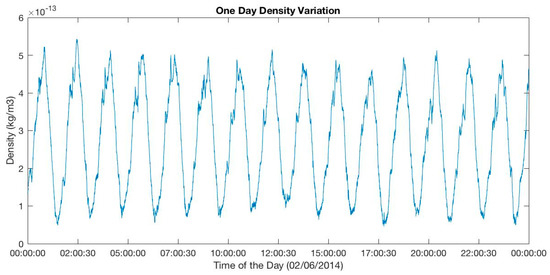
Figure 1.
Diurnal density variation on 2nd June 2014. The unit of density is kg/m3. Time format is shown as HH:SS:MM.
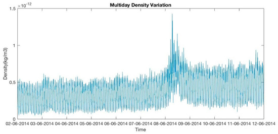
Figure 2.
Same as Figure 1 but for multi–day variation.
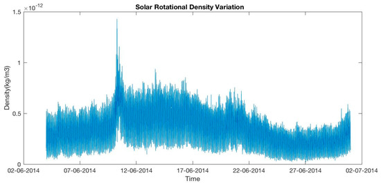
Figure 3.
Same as Figure 1 but for solar rotational variation.
We presented a scalogram analysis to see how F10.7 echo cycle (fluctuation) frequency varies in density over a month. This analysis is important in time series analysis for climate/atmospheric science by comparing variables in wavelet analysis. The relationship between echo frequency and density over time is shown in Figure 4. We can see a significant echo cycle of 2–3 days. The variation can be due to the forcing from the lower atmosphere, for example, planetary/Rossby waves can modulate the multiday variation. Additionally, the arrival and withdrawal of Sun active regions play an important role in modulation.
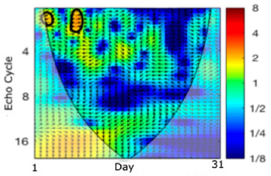
Figure 4.
Scalogram between F10.7 echo cycle frequency and density variation over a month (June 2014). Left (right) pointing arrows indicate that the two (antiphase) signals are in phase and down (up)–pointing arrows indicate that the density fluctuates (does not fluctuate). The density is constant, which does not fluctuate. If an arrow directs horizontally, then the density doesn’t fluctuate.
Figure 5 and Figure 6 show the semi–annual and annual density variation in the upper thermosphere from 2nd June 2014. In September, we can see only a local peak, the seasonal maximum is observed in December–January, whereas the lowest is seen from May to August. The other peak is seen in March 2015. St Patrick’s Day is on 17 March and a storm occurred on that particular date. The density variations follow the “V” shape for the first 2–3 months due to the 27–day solar rotational period and recurrent geomagnetic forcing. Thermospheric density strongly varies seasonally where the large dispersion is detected near the equinoxes whereas the minimum is recorded at the time of northern and southern hemisphere summer. Several researchers have detected the annual density variation. Bowman et al. [5,6] found this variation under high solar activity conditions and the impact of solar indices. Emmert and Picone [16] found the variation due to the F10.7 index and the Kp geomagnetic activity index. Qian and Solomon [12] detected this variation due to eddy mixing comprised by breaking the gravity waves on the mesosphere and lower thermosphere zonal mean winds, which can modify the thermosphere neutral composition.
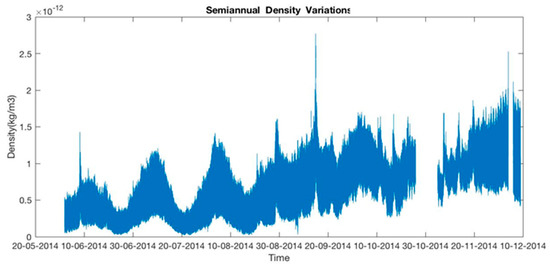
Figure 5.
Same as Figure 1 but for semi–annual variation. The gap in this figure shows the missing data from the Swarm mission.
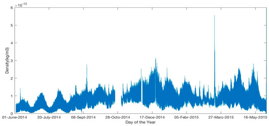
Figure 6.
Same as Figure 5 but for annual variation.
The scalogram analysis is shown again in Figure 7 but considering a year where we can see a significant echo cycle near 3–4 months. This can happen because of missing data that were interpolated.
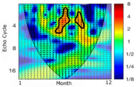
Figure 7.
Same as Figure 4 but for a year.
3.2. Relationship between Annual Density Variation and Solar/Geomagnetic Index
Figure 8 shows the minimum density, which is seen in July, whereas the maximum is observed from September to February. This density variation relates to the distance between the Sun and Earth, which follows the perihelion and aphelion. During perihelion (passed near 4 January), the Earth comes closest to the Sun, and as such we see the highest density in January. On the other hand, the Earth is far from the Sun during aphelion time (close to 4 July), where the minimum density is seen in July. Figure 8 and Figure 9 show the F10.7 and Kp effect on density variations where the strong correlation (r = 0.74) for F10.7 and medium correlation (r = 0.57) for Kp have been calculated, which concludes that some of these characteristics and thermosphere density are driven by solar rotation and its periodical effects, such as the occurrence of the sunspots and strength of the solar flux.
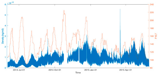
Figure 8.
Density and F10.7 variations over a year. Blue and orange colors represent density and F10.7. F10.7 is presented in the so–called solar flux units, sfu, equal to 10−22 W/(m2∙Hz).
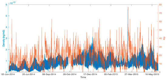
Figure 9.
Same as Figure 8 but for Kp (multiplied by 10).
4. Discussions and Summary
Geomagnetic storms induced thermospheric mass density variations are still challenging because of limited observations and imprecise models. Recently, Swarm satellites have been able to estimate thermospheric mass density variations, and their provided data can be helpful to study thermospheric mass density variations [51].
In this study, we discussed the temporal variations of thermospheric density. The thermospheric density varies seasonally and shows a more complicated pattern than maxima near equinoxes and minima near solstices. Thermospheric empirical models describe the mechanism of the variation; however, the mechanisms are not well agreed. We found a strong correlation (0.74) between annual variation and F10.7, whereas a medium correlation (0.57) was observed between annual data and Kp. We also found the correlation coefficients are significant at 95% confidence level. This is consistent with the study by Guo et al. [52]. They found that among the chosen solar proxies, F10.7 shows the highest correlations with the density for short–term (27 d) variations. For both long–term (>27 d) and short–term variations, linear correlation coefficients exhibit a decreasing trend from low latitudes toward high latitudes.
A significant temperature increase in the auroral region occurred due to strong Joule and particle heating. A geomagnetic storm occurred on 17 March 2015 and showed such a feature where we can see the peak value of the Kp index on 17 March 2015 is 80. During this intense storm, storm time meridian wind influences strong Joule and particle heating in the high–latitude ionosphere and thermosphere. Strong temperature variations are seen due to Joule and particle heating during geomagnetic storms [51].
During a magnetic storm, the energy in the thermosphere can be transferred from high to low latitudes through both gravity waves and meridional circulation. Moreover, disturbances in the high–latitude region propagate equatorward through atmosphere circulation, reaching the middle and lower latitudes in a few hours. Two density peaks are located at around 0 h and 12 h UT during the geomagnetic storm, where the average atmospheric density on the dayside is significantly higher than that on the nightside, and the short–term variations are well correlated with the geomagnetic indices. The thermospheric density rapidly increases during the main phase of the geomagnetic storm, density enhancements are seen during geomagnetic storms and afterward, the enhancements will propagate to lower latitudes due to density gradients, meridional winds, and gravity waves. Swarm observations show symmetric mass density variations, which are expectable according to the solar radiation [53]. The solar rotation cycle in the solar irradiance is a manifestation of the spatial inhomogeneity in the distribution of the bright/dark features on the solar surface and differential rotation of the Sun [54].
The target of numerical and empirical modeling is to understand the mechanism and influence of solar and magnetic activity. The mechanism has been characterized by the seasonal performance of the thermosphere and these seasonal changes detected by various categories of satellite missions; however, the mechanism for variations is still under research [17]. In short, the internal neutral dynamics, thermospheric external forcing, coupling in the thermosphere and ionosphere, and the lower and middle atmosphere’s effects modulate these variations [55]. The diurnal variation is modulated by solar irradiance and multi–day variation is caused by the geomagnetic activity. Furthermore, the arrival and departure of the active regions of the sun caused the solar–rotational variation. Finally, the semi–annual and annual variation is driven by the large–scale circulation and geomagnetic and eddy mixing.
Author Contributions
Conceptualization, A.Y. and M.W.; Methodology, A.Y. and M.W.; Software, A.Y. and M.W.; Validation, A.Y. and M.W.; Formal Analysis, A.Y. and M.W.; Writing—Original Draft Preparation, A.Y. and M.W.; Writing—Review & Editing, M.W.; A.Y.; J.-J.L.; M.A.A.; M.B. and Z.Q. Visualization, A.Y. and M.W.; Funding Acquisition, M.W.; A.Y. and J.-J.L. All authors have read and agreed to the published version of the manuscript.
Funding
M.W. has been supported by Nanjing University of Information Science and Technology Postdoctoral Fellowship, China. SERC limited, Australia supported A.Y. and J.-J.L. is supported by “The Startup Foundation for Introducing Talent of NUIST”.
Conflicts of Interest
The authors declare no conflict of interest.
References
- Forbes, J.M.; Lu, G.; Bruinsma, S.; Nerem, S.; Zhang, X. Thermosphere density variations due to the 15– 24 April 2002 solar events from CHAMP/STAR accelerometer measurements. J. Geophys. Res. 2005, 110, A12S27. [Google Scholar] [CrossRef]
- Amm, O.; Vanhamäki, H.; Kauristie, K.; Stolle, C.; Christiansen, F.; Haagmans, R.; Masson, A.; Taylor, M.G.G.T.; Floberghagen, R.; Escoubet, C.P. A method to derive maps of ionospheric conductances, currents, and convection from the SWARM multisatellite mission. J. Geophys. Res. 2015, 120, 3263–3282. [Google Scholar] [CrossRef]
- Marcos, F.; Garrett, H.; Champion, K.; Forbes, J. Density variations in the lower thermosphere from analysis of the AE–C accelerometer measurements. Planet. Space Sci. 1977, 25, 499–507. [Google Scholar] [CrossRef]
- Marcos, F.; Forbes, J. Thermospheric winds from the satellite electrostatic triaxial accelerometer system. J. Geophys. Res. 1985, 90, 6543–6552. [Google Scholar] [CrossRef]
- Bowman, B.R.; Tobiska, W.K.; Marcos, F.A.; Huang, C.Y.; Lin, C.S.; Burke, W.J. A new empirical thermospheric density model JB2008 using new solar and geomagnetic indices. In Proceedings of the AIAA/AAS Astrodynamics Specialist Conference and Exhibit, Honolulu, HI, USA, 18–21 August 2008; p. 6438. [Google Scholar]
- Bowman, B.R.; Tobiska, W.K.; Marcos, F.A.; Valladares, C. The JB2006 empirical thermospheric density model. J. Atmos. Solar–Terres. Phys. 2008, 70, 774–793. [Google Scholar] [CrossRef]
- Doornbos, E.; Förster, M.; Fritsche, B.; Helleputte, T.; IJssel, I.; Koppenwallner, H.; Rees, D.; Visser, P. Air density models derived from multi–satellite drag observations. In DEOS/TU Delft Scientific Report; Delft University of Technology: Delft, The Netherlands, 2009; p. 27. [Google Scholar]
- Friis–Christensen, E.; Luhr, H.; Knudsen, D.; Haagmans, R. SWARM—An Earth Observation Mission investigating Geospace. Adv. Space Res. 2008, 41, 210–216. [Google Scholar] [CrossRef]
- Olsen, N.; Alken, P.; Beggan, C.; Chulliat, A.; Doornbos, E.; Encarnacao, J.; Floberghagen, R.; Friis–Christensen, E.; Hamilton, B.; Hulot, G.; et al. SCARF—The SWARM Satellite Constellation Application and Research Facility. In Proceedings of the European Space Agency Living Planet Symposium 2013, Edinburgh, UK, 9–13 September 2013; p. 12. [Google Scholar]
- Sang, J.; Smith, C.; Zhang, K. A Method of estimating atmospheric mass density from precision orbit solution. In Proceedings of the AIAA/AAS Astrodynamics, Minneapolis, MO, USA, 13–16 August 2012; pp. 1–7. [Google Scholar]
- Solomon, S.C.; Qian, L.; Didkovsky, L.V.; Viereck, R.A.; Woods, T.N. Causes of low thermospheric density during the 2007–2009 solar minimum. J. Geophys. Res. 2011, 116, A00H07. [Google Scholar] [CrossRef]
- Qian, L.; Solomon, S.C. Thermospheric Density: An Overview of Temporal and Spatial Variations. Space Sci. Rev. 2012, 168, 147–173. [Google Scholar] [CrossRef]
- Sassi, F.; Boville, B.A.; Kinnison, D.; Garcia, R.R. The effects of interactive ozone chemistry on simulations of the middle atmosphere. Geophys. Res. Lett. 2005, 32, L07811. [Google Scholar] [CrossRef]
- Emmert, J.T.; Picone, J.M.; Lean, J.L.; Knowles, S.H. Global change in the thermosphere: Compelling evidence of a secular decrease in density. J. Geophys. Res. 2004, 109, A02301. [Google Scholar] [CrossRef]
- Emmert, J.T.; Drob, D.P.; Shepherd, G.G.; Hernandez, G.; Jarvis, M.J.; Meriwether, J.W.; Niciejewski, R.J.; Sipler, D.P.; Tepley, C.A. DWM07 global empirical model of upper thermospheric storm–induced disturbance winds. J. Geophys. Res. 2008, 113, A11319. [Google Scholar] [CrossRef]
- Emmert, J.T.; Picone, J.M. Climatology of globally averaged thermospheric mass density. J. Geophys. Res. Space Phys. 2010, 115. [Google Scholar] [CrossRef]
- Emmert, J.T. Thermospheric mass density: A review. Adv. Space Res. 2015, 56, 773–824. [Google Scholar] [CrossRef]
- Hedin, A.E. A revised thermospheric model based on mass spectrometer and in coherent scatter data—MSIS–83. J. Geophys. Res. 1983, 88, 10170–10188. [Google Scholar] [CrossRef]
- Hedin, A.E. MSIS–86 thermospheric model. J. Geophys. Res. 1987, 92, 4649–4662. [Google Scholar] [CrossRef]
- Hedin, A.E. The atmospheric model in the region 90 to 2000 km. Adv. Space Res. 1988, 8, 19–25. [Google Scholar] [CrossRef]
- Hedin, A.E. Extension of the MSIS thermospheric model into the middle and lower atmosphere. J. Geophys. Res. 1991, 96, 1159–1172. [Google Scholar] [CrossRef]
- Richmond, A.D.; Ridley, E.C.; Roble, R.G. A thermosphere/ionosphere general circulation model with coupled electrodynamics. Geophys. Res. Lett. 1992, 19, 601–604. [Google Scholar] [CrossRef]
- Peymirat, C.; Richmond, A.D.; Emery, B.A.; Roble, R.G. A magnetosphere– thermosphere–ionosphere electrodynamics general circulation model. J. Geophys. Res. 1998, 103, 17467–17477. [Google Scholar] [CrossRef]
- Roble, R.G.; Ridley, E.C.; Richmond, A.D.; Dickinson, R.E. A coupled thermosphere/ionosphere general circulation model. Geophys. Res. Lett. 1988, 15, 1325–1328. [Google Scholar] [CrossRef]
- Roble, R. On the feasibility of developing a global atmospheric model extending from the ground to the exosphere. Geophys. Mon. 2000, 123, 53–68. [Google Scholar]
- Visser, P.; Doornbos, E.; IJssel, J.; Encarnacao, J.T. Thermospheric density and wind retrieval from SWARM observations. Earth Planets Space 2013, 65, 1319–1331. [Google Scholar] [CrossRef]
- Picone, J.M.; Hedin, A.E.; Drob, D.P.; Aikin, A.C. NRLMSISE–00 empirical model of the atmosphere: Statistical comparisons and scientific issues. J. Geophys. Res. 2002, 107, A12. [Google Scholar] [CrossRef]
- Doornbos, E.; Ijssel, J.; Luhr, H.; Forster, M.; Koppenwallner, G. Neutral density and crosswind determination from arbitrarily oriented multiaxis accelerometers on satellites. J. Space. Rock. 2010, 47, 580–589. [Google Scholar] [CrossRef]
- Wahiduzzaman, M.; Yeasmin, A. Seasonal Statistical forecasting of tropical cyclone landfall activities over the North Indian Ocean rim countries. Atmos Res. 2019, 227, 89–100. [Google Scholar] [CrossRef]
- Wahiduzzaman, M.; Yeasmin, A.; Luo, J.J. Seasonal movement prediction of tropical cyclone over the North Indian Ocean by using atmospheric climate variables in statistical models. Atmos. Res. 2020, 245, 105089. [Google Scholar] [CrossRef]
- Maraun, D.; Kurths, J. Cross wavelet analysis: Significance testing and pitfalls. Nonlinear Process. Geophys. 2004, 11, 505–514. [Google Scholar] [CrossRef]
- Torrence, C.; Compo, G.P. A practical guide to wavelet analysis. Bull. Am. Meteorol. Soc. 1998, 79, 61–78. [Google Scholar] [CrossRef]
- Araghi, A.; Mousavi, B.M.; Adamowski, J.; Malard, J.; Nalley, D.; Hasheminia, S.M. Using wavelet transforms to estimate surface temperature trends and dominant periodicities in Iran based on gridded reanalysis data. Atmos. Res. 2015, 155, 52–72. [Google Scholar] [CrossRef]
- Joshi, N.; Gupta, D.; Suryavanshi, S.; Adamowski, J.; Madramootoo, C.A. Analysis of trends and dominant periodicities in drought variables in India: A wavelet transform based approach. Atmos. Res. 2016, 182, 200–220. [Google Scholar] [CrossRef]
- Goyal, M.K.; Sharma, A. Wavelet transform based trend analysis for drought variability over stations in India. Eur. Water 2017, 60, 247–253. [Google Scholar]
- Pan, F.; Smerdon, J.E.; Stieglitz, M.; Webster, P. A wavelet approach to reconstructing near–surface temperature time series from observations of subsurface temperatures at several meters depth. In AGU Fall Meeting Abstracts; American Geophysical Union: San Francisco, CA, USA, 2005. [Google Scholar]
- Westra, S.; Sharma, A. Dominant modes of interannual variability in Australian rainfall analyzed using wavelets. J. Geophys. Res. 2006, 111. [Google Scholar] [CrossRef]
- Karthikeyan, L.; Nagesh Kumar, D. Predictability of nonstationary time series using wavelet and EMD based ARMA models. J. Hydrol. 2013, 502, 103–119. [Google Scholar] [CrossRef]
- Sang, Y.; Singh, V.; Sun, F.; Chen, Y.; Liu, Y.; Yang, M. Wavelet–based hydrological time series forecasting. J. Hydrol. Eng. 2016, 21, 06016001. [Google Scholar] [CrossRef]
- Kang, S.; Lin, H. Wavelet analysis of hydrological and water quality signals in an agricultural watershed. J. Hydrol. 2007, 338, 1–14. [Google Scholar] [CrossRef]
- Smith, L.C.; Turcotte, D.L.; Isacks, B.L. Stream flow characterization and feature detection using a discrete wavelet transform. Hydrol. Process. 1998, 12, 233–249. [Google Scholar] [CrossRef]
- Bayazit, M.; Onoz, B.; Aksoy, H. Nonparametric streamflow simulation by wavelet or Fourier analysis. Hydrol. Sci. J. 2001, 46, 623–634. [Google Scholar] [CrossRef]
- Labat, D.; Ababou, R.; Mangin, A. Rainfall–runoff relations for karstic springs. Part II: Continuous wavelet and discrete orthogonal multiresolution analyses. J. Hydrol. 2000, 238, 149–178. [Google Scholar] [CrossRef]
- Dieppois, B.; Diedhiou, A.; Durand, A.; Fournier, M.; Massei, N.; Sebag, D.; Xue, Y.; Fontaine, B. Quasi–decadal signals of Sahel rainfall and West African monsoon since the mid–twentieth century. J. Geophys. Res. 2013, 118, 12–587. [Google Scholar] [CrossRef]
- Wahiduzzaman, M.; Luo, J.J. A statistical analysis on the contribution of El Niño–Southern Oscillation to the rainfall and temperature over Bangladesh. Meteorol. Appl. Phys. 2020. [Google Scholar] [CrossRef]
- Ozger, M.; Mishra, A.K.; Singh, V.P. Estimating Palmer Drought Severity Index using a wavelet fuzzy logic model based on meteorological variables. Int. J. Climatol. 2011, 31, 2021–2032. [Google Scholar] [CrossRef]
- Özger, M.; Mishra, A.K.; Singh, V.P. Long lead time drought forecasting using a wavelet and fuzzy logic combination model: A case study in Texas. J. Hydrometeorol. 2012, 13, 284–297. [Google Scholar] [CrossRef]
- Ujeneza, E.L.; Abiodun, B.J. Drought regimes in Southern Africa and how well GCMs simulate them. Clim. Dyn. 2014, 44, 1595–1609. [Google Scholar] [CrossRef]
- Wang, H.; Chen, Y.; Pan, Y.; Li, W. Spatial and temporal variability of drought in the arid region of China and its relationships to teleconnection indices. J. Hydrol. 2015, 523, 283–296. [Google Scholar] [CrossRef]
- Madhu, S.; Kumar, T.L.; Barbosa, H.; Rao, K.K.; Bhaskar, V.V. Trend analysis of evapotranspiration and its response to droughts over India. Theor. Appl. Climatol. 2015, 121, 41–51. [Google Scholar] [CrossRef]
- Zhang, Y.; Paxton, L.J.; & Schaefer, R.K. Deriving thermospheric temperature from observations by the global ultraviolet imager on the thermosphere ionosphere mesosphere energetics and dynamics satellite. J. Geophys. Res. 2019, 124, 5848–5856. [Google Scholar] [CrossRef]
- Guo, J.; Wan, W.; Forbes, J.M.; Sutton, E.; Nerem, R.S.; Woods, T.N.; Bruinsma, S.; Liu, L. Effects of solar variability on thermosphere density from CHAMP accelerometer data. J. Geophys. Res. 2007, 112, A10308. [Google Scholar] [CrossRef]
- Yuan, L.; Jin, S.; Calabia, A. Distinct thermospheric mass density variations following the September 2017 geomagnetic storm from GRACE and Swarm. J. Atmos. Sol. –Terres Phys. 2019, 184, 30–36. [Google Scholar] [CrossRef]
- Shapiro, A.V.; Rozanov, E.; Egorova, T.; Shapiro, A.I.; Peter, T.; Schmutz, W. Sensitivity of the Earth’s middle atmosphere to short–term solar variability and its dependence on the choice of solar irradiance data set. J. Atmos. Sol. –Terres Phys. 2011, 73, 348–355. [Google Scholar] [CrossRef]
- Qian, L.; Solomon, S.C.; Kane, T.J. Seasonal variation of thermospheric density and composition. J. Geophys. Res. 2009, 114, A01312. [Google Scholar] [CrossRef]
© 2020 by the authors. Licensee MDPI, Basel, Switzerland. This article is an open access article distributed under the terms and conditions of the Creative Commons Attribution (CC BY) license (http://creativecommons.org/licenses/by/4.0/).