Abstract
In this work, a comprehensive methodology for trend investigation in rainfall time series, in a climate-change context, is proposed. The crucial role played by a Stochastic Rainfall Generator (SRG) is highlighted. Indeed, SRG application is particularly suitable to obtain rainfall series that are representative of future rainfall series at hydrological scales. Moreover, the methodology investigates the climate change effects on several timescales, considering the well-known Mann–Kendall test and analyzing the variation of probability distributions of extremes and hazard. The hypothesis is that the effects of climate changes could be more evident only for specific time resolutions, and only for some considered aspects. Applications regarded the rainfall time series of the Viterbo rain gauge in Central Italy.
1. Introduction
Climate changes and their impacts on agriculture, industry, economy, human health and ecosystems constitute an always more important topic for the scientific community. Consequently, Climate Change Adaptation (CCA) and Disaster Risk Reduction (DRR) are nowadays a worldwide priority, in order to have resilient societies. Concerning hydraulic and geological risks, heavy rainfall events characterized by high intensity and short duration, and the consequent floods and landslides, increased in many parts of the world, and they are expected to increase further in the future.
In general, the investigation of climate change effects on rainfall series at hydrological scale can be carried out as follows [1]. For past conditions, it is possible to analyze possible trends only for long-term observed time series. For future conditions, the evaluation of changes in rainfall statistics is based on extrapolation from historical records, or on future scenarios simulated by using climatic models and hypothesizing different greenhouse gas emissions.
Concerning observed time series and regarding trend detection in extreme rainfall, many studies were carried out on data recorded at a daily timescale [2]. Such data are not so suitable for hydrological contexts, because sub-daily (and in particular sub-hourly) scales are of main interest for the analysis of flash floods and shallow landslides, in particular for small catchments that present short response times of runoff to rainfall. Only a few studies have focused on the detection of trends in sub-daily data series for large areas [3]. Overall, trends in historical series of meteorological data were usually investigated with parametric and non-parametric approaches [4]. The non-parametric Mann–Kendall (MK) statistical test [5,6] was frequently used to quantify the significance of trends in precipitation time series [7,8,9] and it was widely recommended by the World Meteorological Organization (WMO) [10]. Moreover, even if the sample size of high resolution series is long enough, the obtained trends from observed data could not be suitable for extrapolation into the future, for two main reasons [11]. First, they could be related to climate variability and not to persistent changes in time. Second, an investigated trend depends on the observation period, so it could be different if the observation period is extended.
To overcome such problems, predictions of future rainfall changes can be carried out by using Regional Climate Models (RCM), but their outputs are mainly available at daily scales, and averaged over large spatial resolutions, so they require statistical downscaling or bias correction methods [1,12] for hydrological analyses. Only very recent RCM applications regarded high resolutions (hourly) and small spatial scales (e.g., [13,14]).
Consequently, in this context of uncertainty, mainly due to the scarcity of high-resolution rainfall observed data with an adequate sample size, the use of Stochastic Rainfall Generators (SRG) appears helpful for a more in-depth analysis of rainfall processes. For instance, they could be used for obtaining perturbed time series that are representative of future rainfall at hydrological scales, which are finer than RCM ones. It is noteworthy that SRG generally present a simple formulation and low computational costs, thus allowing to quickly generating large ensembles of long rainfall time series [15,16].
SRG are usually calibrated by using observed rain gauge data. Then their parameters are perturbed by considering the changes predicted by RCM, under the hypothesis that the statistics of areally averaged rainfall simulated by climate models reflect changes at the point rain gauge scale (e.g., [17,18]). In details, these changes (also named as Change Factors, CF) [19,20] are usually computed as differences (or ratios) between the statistics of simulated (by RCM) rainfall series for two future horizons (i.e., near future, 2035–2064, and far future, 2070–2099), and the control period for the current climate (i.e., 1971–2000). In doing so, they are applied in additive (or multiplicative) way to the statistics of the adopted SRG.
Using a SRG for climate change analyses has been successfully tested for many climate conditions [19,21,22,23]. For instance, Maraun et al. [24] recommended the use of SRG as alternative to bias correction methods on RCM [12], due to their ability to simulate local variability and climate extremes.
In this work, a modified version of the Neyman–Scott Rectangular Pulses model (NSRP, [24,25]) was introduced and used as SRG. The model was calibrated by using Annual Maximum Rainfall (AMR) data, which are usually longer than continuous observed series and allow for a better reconstruction of extreme events [26]. Moreover, the seasonality was modeled in a parsimonious way [27]. The selected case study regarded the rainfall time series of the Viterbo rain gauge in Central Italy.
Specifically, the transient SRG was implemented in an equivalent way with respect to CF methodology. We hypothesized mathematical functions representing possible trends for NSRP parameters (which are strongly related to finest scales) on the whole considered future horizon (i.e., 100 years), and then we focused on the best equations that provided comparable results with RCM predictions (indeed associated to coarser resolutions), in terms of variation of prefixed statistics in the spatial cells of the selected case study [28]. Obviously, this constitutes a further and not negligible source of uncertainty [29]. In fact, all the successive evaluations depend on the adopted mathematical expression for parameters’ trends and on the assumption that it remains valid for the entire future design period.
From the obtained perturbed synthetic rainfall series, the changes of extreme values distributions at several timescales were investigated, together with the hazard values on prefixed time horizons.
Overall, the aim of this work is to highlight the need of considering a comprehensive framework for trend investigation, in which many timescales are investigated and several methods are used. In fact, the effects of climate changes could be more evident only for specific time resolutions. Moreover, as previously mentioned, the analysis of only the observed time series could be insufficient, so that the use of perturbed synthetic data should be preferred, together with the adoption and comparison of several approaches for checking stationary or not-stationary behaviors.
In detail, the main goals of this study are to investigate if the following assumptions are true:
- The effects of climate changes could be more evident only on specific data time resolutions;
- The analysis of only the observed time series could be insufficient, so that the use of perturbed synthetic data could be preferred, together with the adoption and comparison of several approaches for checking stationary or not-stationary behaviors.
2. Materials and Methods
2.1. Case Study
The selected case study regards the rainfall time series of the Viterbo rain gauge, located in Lazio region, Central Italy (Figure 1). The rainfall data (provided by ‘Agenzia Regionale di Protezione Civile—Centro Funzionale Regionale’ of Lazio region) consist of Annual Maximum Rainfall (AMR) series of different sub-daily durations (1, 3, 6, 12, and 24 h) with a sample size N = 71 years. Moreover, a continuous high-resolution (5 min) rainfall series from 1994 to 2015 is available, from which the AMR series related to 5, 15 and 30 min were obtained, with N = 22 years.
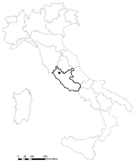
Figure 1.
Viterbo rain gauge (black circle); Lazio region (black polygon) and border of Italy (gray polygon).
2.2. Overview of the Adopted SRG Model
Many works [25,30,31,32,33,34,35] remarked the ability of a specific class of SRG, the Poisson cluster models, to satisfactorily reproduce the observed summary statistics (such as mean, variance, skewness, proportion of dry/wet periods, and k-lag autocorrelation values) of the continuous rainfall process at fine timescale. This class includes the well-known Neyman–Scott and Bartlett–Lewis families, which perform equally well [36] and that were applied in many countries (see [27] for a list of references).
In this work, the single-site Neyman–Scott Rectangular Pulses (NSRP [25,26]) model was considered, which is based on the following assumptions related to a clustering approach (see also Figure 2):
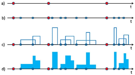
Figure 2.
From De Luca and Galasso [27]. Representation of the Neyman–Scott Rectangular Pulses (NSRP) stochastic process for at-site rainfall modeling: (a) occurrences of storms (Equation (1)); (b) for each storm, determination of the number of pulses (Equation (2)) and their temporal occurrences (Equation (3)); (c) estimation of intensity and duration for all the pulses (Equations (4) and (5)); (d) calculus of total intensity at time, t, calculated as the sum of the intensities which are related to the active bursts at time, t.
- Five quantities play a crucial role in an NSRP model: (i) the inter-arrival time () between the origins of two consecutive storms; (ii) the number, , of rain cells (also indicated as bursts or pulses) inside a specific storm; (iii) the waiting time, , between a specific burst origin and the origin of the associated storm; (iv) the intensity, ; and (v) the duration, , of a specific burst, having a rectangular shape, belonging to a storm.
- , , , and are assumed as random variables, following assigned probability distributions (below described), and then synthetic rainfall series can be generated in stochastic way as reported in the following:
- (a)
- The inter-arrival time (Ts) between the origins of two consecutive storms is assumed as an independent and identically distributed random variable, following an exponential distribution:where is the probability to have a new storm origin after a waiting time from the previous one, and represents the mean value for the inter-arrival times, i.e., . According to the usual notation in statistics, capital letters refer to the random variables, while lowercase letters represent particular values assumed by the random variables. Consequently, is a specific value that can be assumed by . Moreover, the symbol refers to the expected value, i.e., the mean value for a specific variable.
- (b)
- The number, , of rain bursts is usually set as geometric or Poisson distributed. In this work, a geometric distribution is considered with a mean value , and, with the goal of having at least one burst for each storm, the random variable is adopted, with a mean value :
- (c)
- The waiting time, , is assumed as an exponentially distributed variable with parameter and mean value :
- (d)
- The intensity, , and the duration, , of each rectangular burst are both considered as exponentially distributed, with parameters and , respectively, and mean values , :
- (e)
- The total precipitation intensity, , at time, t, is then calculated as the sum of the intensities which are related to the active bursts at time, t (see also Figure 2d and [27]);
- (f)
- Then, the aggregated process, i.e., the rainfall height cumulated on the temporal resolution and related to the time interval j with extremes and , is as follows:
This basic version of a NSRP model has a five-parameter set that is usually calibrated by minimizing an objective function, which is defined as the sum of residuals (normalized or not) between the considered (by user) statistical properties of the observed data at chosen time resolutions and their theoretical expressions. The statistical properties are typically referred to a high-resolution continuous time series (e.g., 1 or 5 min rainfall time series): Mean, variance, and k-lag autocorrelation for at several values of [37] can be mentioned as examples.
However, continuous high resolution datasets are typically very short (in general no more than 15–20 years, and hence not very suitable for obtaining robust estimations) or absent in many locations, where only AMR data are usually available with an adequate sample size.
Moreover, many studies remarked the inability of the SRG like NSRP to reproduce extreme events, because they usually underestimate the rainfall heights at hourly and sub-hourly scales (e.g., [38]). For this reason, many variants of model structure were proposed in the literature [35,39,40,41,42,43,44], but in any case the calibration was carried out by using continuous high resolution datasets and the improvement on reconstruction of extreme events was not significant.
To overcome these critical aspects, the possibility to calibrate the SRG by using only AMR data was investigated in [27,28]; this choice clearly allowed for a better reconstruction of extreme events, which are usually of main interest in many hydrological studies.
Moreover, De Luca et al. [28] proposed a parsimonious modeling of seasonality, adopted in this work, for a basic version of a NSRP model. The goal is to avoid an over parameterization that could occur using monthly or seasonal parameter sets.
In details, due to the fact that the information about the seasonality of the rainfall process during the year is lost with the use of AMR series, a trigonometric series can be defined for any summary statistic of interest for NSRP :
where is the summary statistic along the time t (expressed in min); is the mean value of on the whole year; K is the maximum number of trigonometric functions (also named as harmonics) to be considered; n is the n-th harmonic function; is total number of minutes on the whole year (considered with 365 days); corresponds to the amplitude for the n-th harmonic function; and corresponds to the phase shift for the n-th harmonic function.
The proposed approach is very flexible, because the user can choice to use Equation (7) only for some summary statistics (and the remaining ones are assumed as constant along the time) or for all. Adoption of Equation (7) implies the estimation of 1 + 2K parameters for each summary statistic, i.e., the annual mean value and the K couples regarding amplitude and phase shift.
Under the assumption that seasonal variation regards all five of the summary statistics, the proposed SRG is characterized by 15 parameters if K = 1 for all, 25 parameters if K = 2 for all, 35 parameters if K = 3 for all and so on. Obviously, K can be different from a summary statistic to the other. Moreover, it can be noted that the number of requested parameters makes this SRG parsimonious with respect to the version in which 12 monthly sets should be estimated (i.e., 60 parameters).
In this work, as also specified in Section 3, for the selected case study, it was sufficient to adopt for a seasonal variation with only one harmonics, i.e., K = 1 in Equation (7), while other summary statistics were considered as constant along the year, that means K = 0 for these in Equation (7).
Thus, Equation (7) was applied as follows for :
where is the annual mean value of the summary statistic (i.e., in Equation (7)); , in which is the minimum value of the summary statistic along the year; and is the phase shift for the harmonic function.
Consequently, this SRG presents 7 parameters to be estimated () under the hypothesis of a rainfall process without trends.
In the next subsections, the methodologies about calibration of the stationary model and the subsequent trend modeling are discussed.
2.2.1. Calibration Methodology Without Parameter Trend
De Luca and Galasso [27] proposed a calibration methodology for a stationary SRG when the sample size of AMR series is significantly long for sub-hourly resolutions. In their work, the Authors did not model the seasonality. Although such hypothesis could seem unrealistic, it is coherent with the extreme values theory [45], in which the assumed probability distributions are derived by considering, inside a fixed temporal block (usually a year), a sequence of values (whence the maximum is extracted) as independent and identically distributed random variables, i.e., without any seasonality feature.
An improvement of the calibration methodology, which is adopted in this study, was used in De Luca et al. [28]. Starting from the assigned ranges of variation for each considered parameter, a pure random generation of 10,000 parameter set for NSRP was carried out. Then, De Luca et al. [28] selected (for the successive elaborations) the set that optimizes an objective function, i.e., that minimizes the differences between observed and modeled statistics for the investigated variables. As well-known in the literature [46], the iterations of a pure random search are completely independent and never use previous information to affect the search strategy. Although this methodology could be time consuming, it clearly allows for investigating the whole hypercube of parameters space and the performances related to many local minima with a very simple algorithm.
In particular, for this work the ranges of variation for NSRP parameters can be fixed as follows [37,47]: [0.002 h−1; 0.01 h−1] for ; [2; 10] for ; [0.02 h−1; 0.5 h−1] for βW; [0.05 h/mm; 0.2 h/mm] for βI and [1 h−1; 10 h−1] for βD. Moreover, the range [2 days; 5 days] is adopted for 1/ and [0, 2π] for (see Equation (8)). Then, ten thousand 7-parameter sets can be randomly generated and, for each hypothesized parameter set, a single 500-year realization of continuous 1 min rainfall heights can be reproduced with the usual Monte Carlo techniques [48]. The 500-year rainfall time series is determined according to the property of ergodicity [49,50] related to a stationary process, from which statistical properties of a very long single stationary series are equal to the statistical properties calculated, for each time interval, from multiple realizations. Thus, for a stationary process, generating only a very long time series provides the same information of analysis from shorter multiple realizations. Consequently, due to the ergodicity property of a stationary process, AMR and annual synthetic series can be extracted from a single long 1-min series and compared with the sample ones.
Authors chose here to calibrate the stationary model by considering the set that optimizes the reproduction of average values for hourly and multi-hourly AMR, plus the Mean Annual Precipitation (MAP). Then, the validation is carried out by comparing the following: (i) sample and theoretical Amount–Duration–Frequency (ADF) curves for hourly and multi-hourly rainfall heights; (ii) sample and theoretical average values of sub-hourly AMR series.
2.2.2. Methodology for Parameter Trend
After the model calibration, some parameters trends, i.e., assumed functions , can be hypothesized. Clearly, a further source of uncertainty is introduced, related to the assumed function linking parameters and the covariate t [29]. In fact, all the successive evaluations depend on the specific mathematical expression for and on the assumption that it remains valid for the entire future investigated period.
In this context, several expressions could be assumed [50]: linear, quadratic, regime shifts, sequence of different forms, etc. In this work, we assumed the following linear expressions:
where is the value of the summary statistics at the beginning of the trend (i.e., it corresponds to the value of the stationary process), is its value after m years and is the rate of increase/decrease in one year.
2.3. Scenarios from RCMs
From projections of RCM for Europe, higher rainfall intensities and longer dry periods are generally expected in the future [2,51,52]. In particular, for each adopted RCM, four scenarios of Representative Concentration Pathways (RCP) of total radiative forcing (i.e., the cumulative measure of human emissions of greenhouse gasses from all sources expressed in W/m2) are commonly used as input: RCP 2.6, RCP 4.5, RCP 6 and RCP 8.5. Moreover, an ensemble average projection from all the RCMs is also derived for each RCP. The obtained outputs show an increase of daily precipitation in many areas in winter season, up to 35% during the 21st century, while in summer season it is expected a decrease, particularly in southern and southwestern areas [53].
Considering Italy, and based on the publication of the Italian Institute for Environmental Protection and Research (ISPRA) [54] that was focused on RCP 4.5 (intermediate emissions) and RCP 8.5 (high emissions), with respect to the reference period 1971–2000, the results of the simulations related to a future period until 2090 are as follows:
- A decrease of the annual cumulative precipitation value. In details, the ensemble mean reduction is 13 mm for RCP 4.5 and 71 mm for RCP 8.5;
- A modest increase for the annual maximum daily rainfall. The ensemble mean is, for both RCP 4.5 and RCP 8.5, an increase of 5–7 mm;
- A significant increase for the waiting time between two consecutive rainfall events. The ensemble mean is 8 days for RCP 4.5, and 16 days for RCP 8.5.
All of these ensemble results, averaged on the whole Italian territory, are also referred to as the spatial cell comprising the Viterbo rain gauge in Central Italy.
2.4. Scenarios Analysis from the Adopted Transient SRG
As already mentioned in the Introduction, an in-depth analysis of perturbed synthetic data, obtained from application the proposed variant of NSRP model, was carried out.
In detail, 500 realizations, each one concerning 101 years of continuous 1 min rainfall heights, were generated with the usual Monte Carlo techniques [48]. The first generated year, denoted as “0”, has the features of the calibrated stationary process, while the successive years are characterized by the assumed parameter trends. In this case, analysis with multiple realizations is necessary as the process is not assumed as stationary in this step, and then investigation of only one long time series is not possible, because ergodicity property cannot be considered.
Then, the associated sub-hourly and hourly AMR series were calculated for each realization, and a comprehensive trend detection was structured, by using the Mann–Kendall (MK) test and the evaluation of Hazard variation, which are briefly described in the following subsections.
2.4.1. The Mann–Kendall Test
The Mann–Kendall (MK) test is a non-parametric test for identifying trends in time-series data and, as previously mentioned, has been recommended widely by the World Meteorological Organization for public application [10]. The test considers the relative magnitudes of sample data rather than the data values themselves, and it does not require the data to follow any particular probability distribution.
In details, the MK statistic, S, is defined as follows:
where corresponds to the sample size, and are two generic sequential data values (with i = 1, 2, n − 1, and j = i + 1, i + 2, …, n), and function assumes the following values:
S is approximately normally distributed with the mean E[S] equal to 0, and the variance V(S) computed as follows:
In Equation (12) n is the number of data, m is the number of tied groups and is the number of ties of extent k. A tied group is a set of sample data having the same value. The standard normal test statistic is then considered, which is computed for n > 10 as follows:
can indicate increasing trends, while can indicate decreasing trends. Moreover, once chosen a specific α significance level and calculated the theoretical quantile , the null hypothesis of no trend is rejected when . For the frequently adopted value of α = 0.05, the null hypothesis of no trend is rejected when .
2.4.2. Hazard Variation
As well-known in the risk-analysis literature [55,56], Hazard, H, is associated to a prefixed value of a variable (hydrological or not), and it corresponds to the probability that the event > occurs at least one time in N years (where N is, for example, the design life of a hydraulic structure). In mathematical terms, Hazard is expressed as follows:
where is the probability associated to no exceedance along the i-th year (I = 1, …, N).
Obviously, we can come to the following conclusions:
- For stationary processes, assumes a constant value , and then Equation (15) can be rewritten as follows:
- For nonstationary processes, depends on the time variation for the NSRP parameter set .
Although analytical expressions of probability distributions do not exist for AMR series from the NSRP model, they can be approximated with an EV1 distribution [57], which also provides a good fit for the AMR sample data in this study (Section 3):
where for the i-th year, and is the reference value for AMR at a specific time-resolution.
Consequently, Equation (14) can be rewritten as follows:
In this context, along the 100-year period of NSRP synthetic data generation (excluding the 0-th year), N is assumed as a moving time window (with obviously N < 100 years), and then the hazard evolution in time, by considering different “starts”, can be calculated as follows:
Starting from the NSRP data series, the adopted procedure for hazard analysis can be schematized in the following steps for each timescale:
- For the i-th year (i = 1, …, 100), the EV1 parameters are estimated with the Maximum-Likelihood technique [48], from the correspondent 500 AMR synthetic values;
- The possibility of using regression formulas for both along the 100-year period is investigated, in order to use these formulas in Equation (18);
- is assumed to be a quantile related to a specific return period, T (e.g., T = 100, 200 years), of the stationary process.
3. Results and Discussion
3.1. NSRP Calibration and Validation of the Stationary Version
First of all, the available datasets for Viterbo rain gauge were analyzed in terms of the following:
- Application of MK test for times series covering the periods 1928–2000 and 1928–2015 for AMR (for Annual Precipitation, the investigated periods were 1916–2000 and 1916–2015). This double-check was aimed at testing the hypothesis of stationary process for periods of different length, and at quantifying the data number to be used for calibrating the stationary version of NSRP;
- Goodness-of-fit for AMR series with EV1 distributions, which constitute a good approximation for AMR from NSRP synthetic data [27], as also remarked in Section 2.4.2. Consequently, a satisfactory EV1 fitting can clearly support the adoption of an NSRP model for the selected case study.
At this step of analysis, sub-hourly AMR series were not investigated, since the sample size has a limited time span (the data are observed since 1994), and the trend evaluation would not have been reliable.
Chronological histograms for the investigated time series are reported in Figure 3. Results from the MK test are schematized in Table 1; the null hypothesis of no trend until 2015 cannot be rejected at 0.05 significance level for all the series, as is less than 1.96 for all the samples, so the whole dataset can be used for calibration of the stationary model.
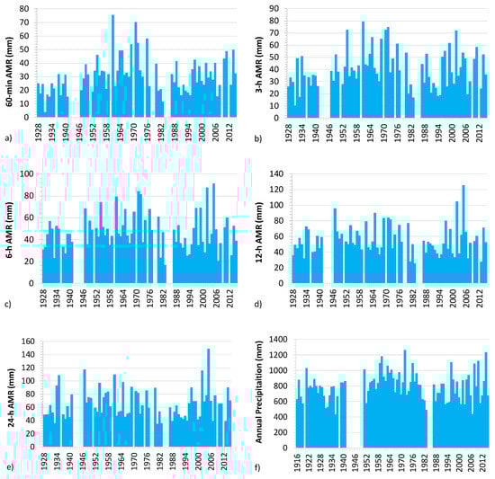
Figure 3.
Viterbo rain gauge: chronological histograms for the investigated time series of Annual Maximum Rainfall (AMR) with durations from 1 to 24 h (a–e) and Annual Precipitation (AP) (f).

Table 1.
Viterbo rain gauge: results of Mann–Kendall (MK) test for the investigated sample time series.
The EV1 probabilistic plots in Figure 4 show the EV1 goodness-of-fit for the hourly AMR sample series, hence confirming the possibility to use the NSRP model.
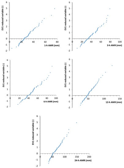
Figure 4.
Viterbo rain gauge: observed AMR series on EV1 probabilistic plots.
As a second step, calibration of the stationary model was carried out as specified in Section 2.2.1, and the results are shown in Table 2. It can be noted that assumes the value equal to π, which means that the mean waiting time 1/λ(t) assumes the minimum value () when t is very close to 0 and Ty (i.e., in the winter period), while its maximum value occurs during the summer season. This result is coherent with the climatology of the Central and Southern Italy [58].
Table 2.
Calibration results of the stationary version of NSRP model for Viterbo rain gauge.
The comparisons among average values for sample and NSRP AMR series (also including sub-hourly series, used for validation) and Annual Precipitation are reported in Table 3.
Table 3.
Viterbo rain gauge: sample and NSRP mean values for the investigated time series.
Moreover, for validation, the comparisons among Amount–Duration–Frequency (ADF) curves obtained from the sample AMR series and those derived from the simulated continuous NSRP process were also carried out. Both sample and NSRP curves were calculated with the common two-parameters ADF formula:
where AMRT(d) is the annual maximum cumulative value for rainfall height (mm), d is the rainfall duration (h), and (mm/h) and (-) are the ADF parameters related to return period T, based on rain gauge observations.
Table 4 reports the estimates for and at prefixed values of return period T for both cases. From Figure 5 we can observe, by applying Equation (19) with parameters in Table 4, a difference of about 2 mm for T = 20 years, about 0.9 mm for T = 50 years, about 0.1 mm per T = 100 years and about 0.6 mm for T = 200 years.
Table 4.
Viterbo rain gauge: sample and NSRP estimates for (mm/h) and (-) Amount–Duration–Frequency (ADF) curves parameters. T is the return period (y).
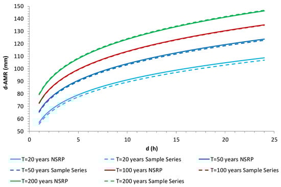
Figure 5.
Viterbo rain gauge: sample and NSRP ADF curves.
3.2. Results of Transient Version for the Proposed NSRP Model
As already mentioned in the Introduction, NSRP parameters are strongly related to finest scales, while RCM predictions are only available for coarser resolutions. Thus, some NSRP parameters trends were hypothesized, and the Authors considered those that provided compatible results with RCM scenarios, in terms of variation for maximum daily rainfall and annual precipitation. In detail, the adopted scenario combines the following hypotheses:
- A linear increasing trend of 50% in 100 years concerning the mean value of Bursts Intensity (i.e., );
- A linear decreasing trend of 25% in 100 years concerning the mean value of Bursts Duration (i.e., );
- A linear increasing trend of 50% in 100 years concerning the mean waiting time between two consecutive storms (i.e., ).
These trends provided a marked variation, in terms of frequency distribution, for AMR series at finer resolutions (5 and 15 min) and for Annual Precipitation, while AMR series at coarser scales seem to be not so influenced by the imposed trends. Some comparisons are shown in Figure 6, in which the frequency distributions for the initial year (t0) and the 25th (t25), the 50th (t50) and the 100th (t100) years are represented.
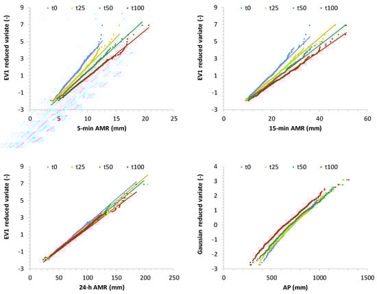
Figure 6.
Viterbo rain gauge: evolution of frequency distributions for some investigated time series.
Focusing on Annual Precipitation (AP) and 24-h AMR series, the temporal evolution of their average values (calculated for each year from the correspondent 500 realizations), compatible with RCM projections, were characterized by the following (Table 5):
Table 5.
Evolution of average values for Annual Maximum Rainfall (AMR) and of Mean Annual Precipitation (MAP): from now (t0) to 25 (t25), 50 (t50), 75 (t75) and 100 (t100) years.
- A mean reduction of 82.5 mm in 100 years obtained for AP (well-matched with 71 mm in 90 years from RCP 8.5);
- A slight increase for 24-h AMR, of about 4 mm in 100 years (the ensemble mean is, for both RCP 4.5 and RCP 8.5, up to 5–7 mm in 90 years, related to daily duration).
Moreover, from Table 5, it can be noted that there is an increase in mean values of about 37% (5 min AMR), 28% (15 min AMR) and 17% (30 min AMR) in 100 years. These differences are lower and less evident for hourly timescales; indeed, the increase in average values is about 5–7% in 100 years.
The results can be justified from the assumed trend scenario:
- An increase in burst intensity induces a clear marked effect (i.e., an expected increase in rainfall height) mainly for finer time resolutions (5–30 min), which are not so influenced by a contemporary reduction of burst duration.
- On the contrary, for coarser resolutions (from 1 h), the simultaneous presence of an increase for intensity and of a reduction in bursts duration produces a sort of balance for rainfall heights, and then it is not possible to highlight a significant trend for AMR series.
- The increase of the average waiting time between two consecutive storms mainly influences the reduction of annual precipitation, as expected from RCM projections.
This “scale effect”, i.e., that there are some particular time resolutions where the assumed temporal changes in parameters could be “hidden” when AMR series are studied, is also confirmed by analyzing the NSRP realizations with MK test.
The histograms in Figure 7 indicate, for each investigated time resolution, the percentage of realizations with Zs > 1.96. The percentages decrease, passing from a 5-min to 1-h time resolution, and are always less than 10% for hourly and multi-hourly AMR synthetic data. Concerning AP, the percentage with Zs > 1.96 is about 30%.
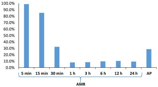
Figure 7.
MK test for Viterbo rain gauge: percentages of synthetic times series with Zs > 1.96, for different timescales.
The results from MK test highlight the importance of analysis with a SRG, and in particular with a large number of simulations. In fact, if a user would consider only one realization for all the investigated scales, he could obtain misleading assessments concerning the presence of trend or not for specific time resolutions. For example, if the considered 3-h AMR series belongs to the subset with Zs > 1.96, then the null hypothesis of no-trend is rejected; on the contrary, using a 15-min AMR series with Zs < 1.96 could imply the null hypothesis is not rejected. Similar considerations could be made if the application of MK test (or other similar tests) is carried out only on the observed series for a selected case study. Then, an overall analysis with a large number of simulations allows for a very in-depth investigation.
Concerning the variation of T-year percentiles and Hazard (Section 2.4.2), the possibility of applying regression formulas for estimated EV1 parameters along the 100-year period was investigated. Coefficients for linear regressions are shown in Table 6, together with the R2 values, which are greater than 0.5, so that the obtained regressions can be considered as acceptable [59]. As examples, the plots for 5- and 15-min EV1 parameters are illustrated in Figure 8.
Table 6.
Estimation of linear regression coefficients (m is the angular coefficient, q is the intercept and R2 is the coefficient of determination) for time evolution of EV1 parameters.
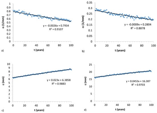
Figure 8.
Linear regressions for time evolution of EV1 parameters, for 5-min (a,c) and 15-min (b,d) AMR synthetic data.
Then, the regression laws were used for quantifying the temporal variation of the following:
- The 100-year and 200-year AMR quantiles with respect to the correspondent values of the stationary process (Figure 9);
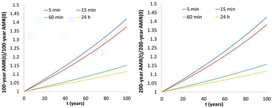 Figure 9. Temporal variation of 100-year (left) and 200-year (right) AMR quantiles with respect to the correspondent values of the stationary process.
 - Hazard (Equation (18)), by considering a 20-year moving time window (Figure 10).
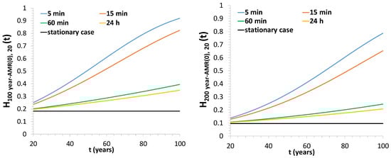 Figure 10. Temporal variation of Hazard related to the 100-year (left) and 200-year (right) AMR quantiles of the stationary process.
The increases are significant for finer resolutions, while they are relatively more limited, but still not negligible, for coarser scales. In details, increases for 24 h quantiles are 11–12% with respect to the stationary case, while they exceed 40% and 35% for the 5 and 15 min scales, respectively.
Hazard values, associated to a 20-year moving window and related to 100-year and 200-year quantiles of the stationary case, are as follows:
- For finer scales (5–15 min), from 10% (T = 100 years) and 18% (T = 200 years) at the beginning of the investigated period, to 60% and 80%, respectively, at the end;
- For 24 h resolutions, 20% (T = 100 years) and 35% (T = 200 years).
Thus, although variations for the investigated 24-h percentiles are relatively modest, the associated hazards at least double if compared with the values assumed at the beginning of the time horizon.
These results highlight the importance of investigation of several aspects before the choice of a stationary or a non-stationary model is made.
However, in a climate change context, it should be remarked the difference between the terms “stationarity” and “change”, and the fact that they are not mutually exclusive [49]. Very popular “examples” can be mentioned [49]. For instance, in the absence of an external force, the position of a body in motion changes in time but the velocity is unchanged (Newton’s first law). If a constant force is present, then the velocity changes but the acceleration is constant (Newton’s second law). If the force changes, e.g., the gravitational force with changing distance in planetary motion, the acceleration is no longer constant, but other invariant properties emerge, e.g., the angular momentum (Newton’s law of gravitation).
Non-stationarity is usually considered as synonymous with change, but change is a general notion applicable everywhere, including the real (material) world, while stationarity and non-stationarity are applied only to models, and not to the real world. Thus, environmental changes can be modeled also with stationary approaches [60] and only in justified cases with non-stationary approaches.
In this specific case study, related to the Viterbo rain gauge in Central Italy, the imposed trends on βI, βD and λ imply the need of using non stationary approaches for the finer time resolutions which are comparable with βD and the annual aggregation (i.e., for MAP evaluation). This is true because a change on the inter-arrival time between two consecutive storms firstly influences monthly and yearly scales (Figure 6).
On the contrary, a stationary modeling could be used for other investigated resolutions, as the temporal variation of the probability distributions seems not so significant. However, a complete analysis including the investigation of hazard and high percentiles makes the use of a non-stationary approach more plausible also for the coarser time resolutions.
4. Conclusions
The results of this work shed new insights on the analysis of climate change effects on rainfall series. The main goal of the applied methodology is understanding if significant trends depend on the investigated timescales. The crucial role in the investigated methodology is played by the use of a Stochastic Rainfall Generator (SRG), which allows users to carry out a very in-depth investigation.
Different sources of uncertainty can arise due to several factors. First, the intrinsic model uncertainty due to the structure of a SRG should be carefully investigated. Second, a further uncertainty can lie in the SRG parameters estimation. Third, the reliability of RCM projections and the assumption of their validity at point scales are questionable. Forth, there is the uncertainty due to the adopted mathematical expression for assessing parameters’ trends and to the assumption that such mathematical expression remains valid for the entire future investigated period. Notwithstanding, the obtained results highlighted that the imposed parameter trends on prefixed time resolutions could imply an “apparent stationarity” of the process and, therefore, that stationary models could be employed, if a user focuses only on some aspects. In fact, for the selected case study, if the AMR probability distributions, derived from simulations with a transient SRG, are analyzed, the associated variations for coarser resolutions are not so significant. This would imply that the use of a stationary model seems to be suitable. Conversely, a more detailed study regarding high percentiles and hazard would allow for us to reconsider a non-stationary approach for all the timescales.
Author Contributions
Conceptualization, D.L.D.L., A.P. and L.G.; methodology, D.L.D.L.; software, D.L.D.L.; validation, D.L.D.L., A.P. and L.G..; data curation, A.P.; writing—original draft preparation, D.L.D.L., A.P. and L.G.; writing—review and editing, D.L.D.L., A.P. and L.G. All authors have read and agreed to the published version of the manuscript.
Funding
This research received no external funding.
Acknowledgments
This work was supported by the Italian Ministry of the Environment, Land and Sea (MATTM) through the project “La mitigazione del rischio idraulico in bacini costieri con casse di espansione in linea: approccio integrato per il dimensionamento”, CUP E68D20000010001.
Conflicts of Interest
The authors declare no conflict of interest.
References
- Willems, P.; Arnbjerg-Nielsen, K.; Olsson, J.; Nguyen, V.T.V. Climate change impact assessment on urban rainfall extremes and urban drainage: Methods and shortcomings. Atmos. Res. 2012, 103, 106–118. [Google Scholar] [CrossRef]
- EEA—European Environment Agency. Climate Change Adaptation ad Disaster Risk Reduction in Europe; EEA: Copenhagen, Denmark, 2017; Volume 15, pp. 1–171. [Google Scholar]
- Hartmannm, D.L.; Klein Tank, A.M.; Rusticucci, M. Observations: Atmosphere and surface. In Climate Change 2013: The Physical Science Basis; Cambridge University Press: Cambridge, UK, 2013. [Google Scholar]
- Sayemuzzaman, M.; Jha, M.K. Seasonal and annual precipitation time series trend analysis in North Carolina, United States. Atmos. Res. 2014, 137, 183–194. [Google Scholar] [CrossRef]
- Mann, H.B. Non-parametric tests against trend. Econometrica 1945, 13, 245–259. [Google Scholar] [CrossRef]
- Kendall, M.G. Rank Correlation Measures; Charles Griffin: London, UK, 1975. [Google Scholar]
- Tabari, H.; Somee, B.S.; Zadeh, M.R. Testing for long-term trends in climatic variables in Iran. Atmos. Res. 2011, 100, 132–140. [Google Scholar] [CrossRef]
- Martinez, J.C.; Maleski, J.J.; Miller, F.M. Trends in precipitation and temperature in Florida, USA. J. Hydrol. 2012, 452–453, 259–281. [Google Scholar] [CrossRef]
- Młyński, D.; Wałęga, A.; Petroselli, A.; Tauro, F.; Cebulska, M. Estimating Maximum Daily Precipitation in the Upper Vistula Basin, Poland. Atmosphere 2019, 10, 43. [Google Scholar] [CrossRef]
- Mitchell, J.M.; Dzezerdzeeskii, B.; Flohn, H.; Hofmeyer, W.L.; Lamb, H.H.; Rao, K.N.; Wallen, C.C. Climatic Change. WMO Technical Note 79, WMO No. 195.TP-100; World Meteorological Organization: Geneva, Switzerland, 1996; p. 79. [Google Scholar]
- Blöschl, G.; Hall, J.; Viglione, A.; Perdigao, R.; Parajka, J.; Merz, B.; Lun, D.; Arheimer, B.; Aronica, G.; Bilibashi, A.; et al. Changing climate both increases and decreases European river floods. Nature 2019, 573, 108–111. [Google Scholar] [CrossRef]
- Maraun, D. Bias Correcting Climate Change Simulations-A Critical Review. Curr. Clim. Change Rep. 2016, 2, 211–220. [Google Scholar] [CrossRef]
- Kendon, E.J.; Roberts, N.M.; Fowler, H.J.; Roberts, M.J.; Chan, S.C.; Senior, C.A. Heavier summer downpours with climate change revealed by weather forecast resolution model. Nat. Clim. Chang. 2014, 4, 570–576. [Google Scholar] [CrossRef]
- Ban, N.; Schmidli, J.; Schär, C. Heavy precipitation in a changing climate: Does short-term summer precipitation increase faster? Geophys. Res. Lett. 2015, 42, 1165–1172. [Google Scholar] [CrossRef]
- Ritschel, C.; Ulbrich, U.; Névir, P.; Rust, H.W. Precipitation extremes on multiple timescales–Bartlett–Lewis rectangular pulse model and intensity–duration–frequency curves. Hydrol. Earth Syst. Sci. 2017, 21, 6501–6517. [Google Scholar] [CrossRef]
- Grimaldi, S.; Petroselli, A.; Piscopia, R.; Tauro, F. The Benefit of Continuous Modelling for Design Hydrograph Estimation in Small and Ungauged Basins. In Innovative Biosystems Engineering for Sustainable Agriculture, Forestry and Food Production; Coppola, A., Di Renzo, G., Altieri, G., D’Antonio, P., Eds.; Springer: Cham, Switzerland, 2020; Volume 67, pp. 133–139. [Google Scholar] [CrossRef]
- Kilsby, C.G.; Jones, P.D.; Burton, A.; Ford, A.C.; Fowler, H.J.; Harpham, C.; James, P.; Smith, A.; Wilby, R.L. A daily weather generator for use in climate change studies. Environ. Model. Softw. 2007, 22, 1705–1719. [Google Scholar] [CrossRef]
- Onof, C.; Arnbjerg-Nielsen, K. Quantification of anticipated future changes in high resolution design rainfall for urban areas. Atmos. Res. 2009, 92, 350–363. [Google Scholar] [CrossRef]
- Blenkinsop, S.; Harpham, C.; Burton, A.; Goderniaux, P.; Brouyère, S.; Fowler, H.J. Downscaling transient climate change with a stochastic weather generator for the Geer catchment, Belgium. Clim. Res. 2013, 57, 95–109. [Google Scholar] [CrossRef]
- Burton, A.; Fowler, H.J.; Blenkinsop, S.; Kilsby, C.G. Downscaling transient climate change using a Neyman-Scott rectangular pulses stochastic rainfall model. J. Hydrol. 2010, 381, 18–32. [Google Scholar] [CrossRef]
- van Vliet, M.T.H.; Blenkinsop, S.; Burton, A.; Harpham, C.; Broers, H.P.; Fowler, H.J. A multi-model ensemble of downscaled spatial climate change scenarios for the Dommel catchment, Western Europe. Clim. Chang. 2012, 111, 249–277. [Google Scholar] [CrossRef]
- Forsythe, N.; Fowler, H.J.; Blenkinsop, S.; Burton, A.; Kilsby, C.G.; Archer, D.R.; Harpham, C.; Hashmi, M.Z. Application of a stochastic weather generator to assess climate change impacts in a semi-arid climate: The Upper Indus Basin. J. Hydrol. 2014, 517, 1019–1034. [Google Scholar] [CrossRef]
- Jones, P.D.; Harpham, C.; Burton, A.; Goodess, C.M. Downscaling regional climate model outputs for the Caribbean using a weather generator. Int. J. Climatol. 2016, 36, 4141–4163. [Google Scholar] [CrossRef]
- Maraun, D.; Shepherd, T.G.; Widmann, M.; Zappa, G.; Walton, D.; Gutiérrez, J.M.; Hagemann, S.; Richter, I.; Soares, P.M.M.; Hall, A.; et al. Towards process-informed bias correction of climate change simulations. Nat. Clim. Chang. 2017, 7, 764–773. [Google Scholar] [CrossRef]
- Rodriguez-Iturbe, I.; Cox, D.R.; Isham, V. Some Models for Rainfall Based on Stochastic Point Processes. Proc. R. Soc. Lond. A Math. Phys. Sci. 1987, 410, 269–288. [Google Scholar]
- Cowpertwait, P.S.P. Further developments of the Neyman-Scott clustered point process for modeling rainfall. Water Resour. Res. 1991, 27, 1431–1438. [Google Scholar] [CrossRef]
- De Luca, D.L.; Galasso, L. Calibration of NSRP Models from Extreme Value Distributions. Hydrology 2019, 6, 89. [Google Scholar] [CrossRef]
- De Luca, D.L.; Petroselli, A.; Galasso, L. Modelling climate changes with stationary models: Is it possible or is it a paradox? In Numerical Computations: Theory and Algorithms; Sergeyev, Y., Kvasov, D., Eds.; Springer: Cham, Switzerland, 2020; Volume 11974. [Google Scholar] [CrossRef]
- Rootzén, H.; Katz, R.W. Design life level: Quantifying risk in a changing climate. Water Resour. Res. 2013, 49, 5964–5972. [Google Scholar] [CrossRef]
- Rodriguez-Iturbe, I.; Cox, D.R.; Isham, V. A Point Process Model for Rainfall: Further Developments. Proc. R. Soc. Lond. A Math. Phys. Eng. Sci. 1998, 417, 283–298. [Google Scholar]
- Onof, C.; Wheater, H.S. Improvements to the modelling of British rainfall using a modified Random Parameter Bartlett-Lewis Rectangular Pulse Model. J. Hydrol. 1994, 157, 177–195. [Google Scholar] [CrossRef]
- Cowpertwait, P.S.P.; O’Connell, P.E.; Metcalfe, A.V.; Mawdsley, J.A. Stochastic point process modelling of rainfall. I. Single-site fitting and validation. J. Hydrol. 1996, 175, 17–46. [Google Scholar] [CrossRef]
- Verhoest, N.; Troch, P.A.; De Troch, F.P. On the applicability of Bartlett–Lewis rectangular pulses models in the modeling of design storms at a point. J. Hydrol. 1997, 202, 108–120. [Google Scholar] [CrossRef]
- Cameron, D.; Beven, K.; Tawn, J. An evaluation of three stochastic rainfall models. J. Hydrol. 2000, 228, 130–149. [Google Scholar] [CrossRef]
- Kaczmarska, J.; Isham, V.; Onof, C. Point process models for fine-resolution rainfall. Hydrol. Sci. J. 2014, 59, 1972–1991. [Google Scholar] [CrossRef]
- Wheater, H.S.; Isham, V.S.; Chandler, R.E.; Onof, C.J.; Stewart, E.J. Improved Methods for National Spatial–Temporal Rainfall and Evaporation Modelling for BSM; Defra: London, UK, 2006. [Google Scholar]
- Cowpertwait, P.S.P. A Poisson-cluster model of rainfall: High-order moments and extreme values. Proc. R. Soc. Lond. 1998, 454, 885–898. [Google Scholar] [CrossRef]
- Verhoest, N.; Vandenberghe, S.; Cabus, P.; Onof, C.; MecaFigueras, T.; Jameleddine, S. Are stochastic point rainfall models able to preserve extreme flood statistics? Hydrol. Process. 2010, 24, 3439–3445. [Google Scholar] [CrossRef]
- Cowpertwait, P. A generalized point process model for rainfall. Proc. R. Soc. A. Math. Phys. 1994, 447, 23–37. [Google Scholar]
- Cameron, D.; Beven, K.; Tawn, J. Modelling extreme rainfalls using a modified random pulse Bartlett–Lewis stochastic rainfall model (with uncertainty). Adv. Water Resour. 2000, 24, 203–211. [Google Scholar] [CrossRef]
- Evin, G.; Favre, A. A new rainfall model based on the Neyman–Scott process using cubic copulas. Water Resour. Res. 2008, 44, W03433. [Google Scholar] [CrossRef]
- Koutsoyiannis, D.; Onof, C. Rainfall disaggregation using adjusting procedures on a Poisson cluster model. J. Hydrol. 2001, 246, 109–122. [Google Scholar] [CrossRef]
- Onof, C.; Townend, J.; Kee, R. Comparison of two hourly to 5-min rainfall disaggregators. Atmos. Res. 2005, 77, 176–187. [Google Scholar] [CrossRef]
- Kossieris, P.; Makropoulos, C.; Onof, C.; Koutsoyiannis, D. A rainfall disaggregation scheme for sub-hourly time scales: Coupling a Bartlett–Lewis based model with adjusting procedures. J. Hydrol. 2018, 556, 980–992. [Google Scholar] [CrossRef]
- Fisher, R.A.; Tippett, L.H.C. Limiting forms of the frequency distribution of the largest or smallest member of a sample. Proc. Camb. Philos. Soc. 1928, 24, 180–290. [Google Scholar] [CrossRef]
- Zabinsky, Z.B. Pure random search and pure adaptive search. In Stochastic Adaptive Search for Global Optimization. Nonconvex Optimization and Its Applications; Springer: Boston, MA, USA, 2003; Volume 72. [Google Scholar] [CrossRef]
- Calenda, G.; Napolitano, F. Parameter estimation of Neyman-Scott processes for temporal point rainfall simulation. J. Hydrol. 1999, 225, 45–66. [Google Scholar] [CrossRef]
- Kottegoda, N.T.; Rosso, R. Applied Statistics for Civil. and Environmental Engineers; Wiley-Blackwell: Hoboken, NJ, USA, 2008; p. 736. ISBN 978-1-405-17917-1. [Google Scholar]
- Koutsoyiannis, D.; Montanari, A. Negligent killing of scientific concepts: The stationarity case. Hydrol. Sci. J. 2014, 60, 1174–1183. [Google Scholar] [CrossRef]
- Serinaldi, F.; Kilsby, C.G. Stationarity is undead: Uncertainty dominates the distribution of extremes. Adv. Water Resour. 2015, 77, 17–36. [Google Scholar] [CrossRef]
- Seneviratne, S.I.; Nicholls, N.; Easterling, D.; Goodess, C.M.; Kanae, S.; Kossin, J.; Luo, Y.; Marengo, J.; McInnes, K.; Rahimi, M.; et al. Changes in climate extremes and their impacts on the natural physical environment. In Managing the Risks of Extreme Events and Disasters to Advance Climate Change Adaptation; Cambridge University Press: Cambridge, UK, 2012; pp. 109–230. [Google Scholar]
- Hov, Ø.; Cubasch, U.; Fischer, E.; Höppe, P.; Iversen, T.; Kvamstø, N.G.; Kundzewicz, Z.W.; Rezacova, D.; Rios, D.; Duarte Santos, F.; et al. Extreme Weather Events in Europe: Preparing for Climate Change Adaptation; Norwegian Meteorological Institute: Oslo, Norway, 2013. [Google Scholar]
- Jacob, D.; Petersen, J.; Eggert, B.; Alias, A.; Christensen, O.; Bouwer, L.; Braun, A.; Collete, A.; Déqué, M.; Georgievski, G.; et al. EURO-CORDEX: New high-resolution climate change projections for European impact research. Reg Environ. Chang. 2014, 14, 563–578. [Google Scholar] [CrossRef]
- Desiato, F.; Fioravanti, G.; Fraschetti, P.; Perconti, W.; Piervitali, E. II Clima Futuro in Italia: Analisi delle Proiezioni dei Modelli Regionali; ISPRA: Roma, Italy, 2015; Volume 58, pp. 1–64. ISBN 978-88-448-0723-8.
- Volpi, E. On return period and probability of failure in hydrology. WIREs Water 2019, 6, e1340. [Google Scholar] [CrossRef]
- Salas, J.D.; Obeysekera, J. Revisiting the Concepts of Return Period and Risk for Nonstationary Hydrologic Extreme Events. J. Hydrol. Eng. 2014, 19, 554–568. [Google Scholar] [CrossRef]
- Marco, J.B.; Harboe, R.; Salas, J.D. Stochastic Hydrology and its Use in Water Resources Systems Simulation and Optimization; Springer: Berlin, Germany, 1993; ISBN 978-94-010-4743-2. [Google Scholar]
- Greco, A.; De Luca, D.L.; Avolio, E. Heavy Precipitation Systems in Calabria Region (Southern Italy): High-Resolution Observed Rainfall and Large-Scale Atmospheric Pattern Analysis. Water 2020, 12, 146. [Google Scholar] [CrossRef]
- Ritter, A.; Muñoz-Carpena, R. Performance evaluation of hydrological models: Statistical significance for reducing subjectivity in goodness-of-fit assessments. J. Hydrol. 2013, 480, 33–45. [Google Scholar] [CrossRef]
- Montanari, A.; Koutsoyiannis, D. Modeling and mitigating natural hazards: Stationarity is immortal! Water Resour. Res. 2014, 50, 9748–9756. [Google Scholar] [CrossRef]
Publisher’s Note: MDPI stays neutral with regard to jurisdictional claims in published maps and institutional affiliations. |
© 2020 by the authors. Licensee MDPI, Basel, Switzerland. This article is an open access article distributed under the terms and conditions of the Creative Commons Attribution (CC BY) license (http://creativecommons.org/licenses/by/4.0/).