Lag Variables in Nitrogen Oxide Concentration Modelling: A Case Study in Wrocław, Poland

Abstract

Due to the unwavering interest of both residents and authorities in the air quality of urban agglomerations, we pose the following question in this paper: What impact do current and past meteorological factors and traffic flow intensity have on air quality? What is the impact of lagged variables on the fit of an explanation model, and how do they affect its ability to predict? We focused on NO₂ and NO_x concentrations, and conducted this research using hourly data from the city of Wrocław (western Poland) from 2015 to 2017; we used multi-objective optimization to determine the optimal delays. It turned out that for both NO₂ and NO_x, the past values for traffic flow, wind speed, and sunshine duration are more important than the current ones. We built random forest models on each of the pollutants for both the current and past values and discovered that including a lagged variable increases the resulting R² from 0.51 to 0.56 for NO₂ and from 0.46 to 0.52 for NO_x. We also analyzed the feature importance in each model, and found that for NO₂, a wind speed delay of more than three hours causes a significant decrease, while the importance of relative humidity increases with a seven-hour delay; likewise, wind speed increases the importance for NO_x prediction with a two-hour delay. We concluded that, in pollutant concentration modeling, the possibility of a delayed effect of the independent variables should always be considered, because it can significantly increase the performance of the model and suggest unexpected relationships or dependencies.

1. Introduction

Harmful air pollution, particularly in densely populated cities, is an unquestionable fact. The growing population of cities and the increasing use of motor vehicles among inhabitants are reasons for the ever-increasing traffic volume and resulting increase in exhaust gas emissions. The expansion of cities and a high density of buildings reduce ventilation in cities. Increased surface roughness results in a decrease in the impact of low wind speeds on the evacuation of pollution. Wrocław currently has 641,600 residents [1]. It is estimated that about 15,000 vehicles move around the city streets every day [2]. One of the main air pollutants emitted by cars’ combustion engines are nitrogen oxides: NO₂ and NO_x (sum of nitrogen oxide and nitrogen dioxide). Studying and measuring the impact of traffic intensity and meteorological factors on the nitrogen oxide concentration in the air of the urban agglomeration provides an opportunity to attempt to manipulate traffic so as to reduce the concentration of pollutants, thereby improving the air quality and the quality of life of the residents. Pollution models can support urban managers in taking action to improve air quality in the city [3,4,5,6].

In the literature, there are several methods for modelling air pollution concentrations. For example, multidimensional regression models are still in use [7,8,9]. The main advantage of linear models is having an interpretable explicit function that can be used to determine the quantitative impact of each predictor on the value of the explaining variable. The extension of linear models includes polynomial forms of functions—in which each variable may be raised to some power [10,11] and non-linear behavior can be taken into account. On the other end of this spectrum, there are models that do not require any assumption about a specific analytical function, also called black-box models, such as artificial neural networks [12,13], or those combined with multiple regression [14], single random trees [15], or more complex structures like random forest (RF) [16,17,18,19,20,21] and boosted regression trees (BRT) [22,23]. These models are more computationally advanced and have been successfully used in pollution concentration modeling.

Zhu et al. [17] developed an RF model based on NO₂ environmental monitoring data and geographical covariates to predict monthly average NO₂ concentration. The RF model shown in this paper reveals performance with a cross validation R² of 0.77 and a root mean square error (RMSE) of 11.0 µgm⁻³. Araki et al. [16] developed a spatiotemporal land use random forest model of the monthly mean NO₂ in metropolitan areas of Japan. The authors obtained an R² value of 0.79. A model using RF methodology in combination with spatiotemporal kriging was developed by Zhan et al. [20] to estimate the daily ambient NO₂ concentrations across China based on satellite retrievals and geographic covariates. The model has a prediction performance R² of 0.62 (RMSE = 13.3 µgm⁻³) for time (daily) and an R² of 0.73 (RMSE = 6.5 µgm⁻³) for spatial predictions. The literature also contains examples of the use of the RF method in combination with techniques other than spatial modeling, for example with the evolving differential evolution method [24]. Kamińska [25] used an RF model to predict daily minimum, average, and maximum daily NO₂ concentrations. The best fit was obtained for a daily average model where ${\mathrm{R}}^2=0.69$, $\mathrm{RMSE}=7.47 \mu \mathrm{g}{\mathrm{m}}^{-2}$, and $\mathrm{MAPE}=11.4\%$. The accuracy of the models generally decreases as the data frequency increases and the research period extends. Increasing the variation in hourly values makes it difficult to predict their values effectively. For hourly data, the typical model fit drops to an R² of around 0.5 [21]. Kamińska [26] carried out a modification of the RF model which improved the quality of fit to R² = 0.82, although there were difficulties predicting future values, and the authors hypothesized that past predictor values may have a greater impact on the current pollution concentration than actual ones.

Studies on the impact of traffic flow and meteorological conditions in Wrocław have already been carried out. In [18], the influence of nine predictors on nitrogen oxide and particulate matter (diameter less than 2.5 µm) concentrations was presented. Nine different models corresponding with nine time-sets of cases were defined, depending on the time for which the analysis was performed. Hourly data (in the years 2015–2016) were considered in one of them. The others were warm and cool (heating) seasons, working and non-working days, and the seasons of the year. The researcher showed that traffic flow intensity has the greatest impact on NO₂ and NO_x concentrations, with engines being the biggest source of emissions. The speed and direction of the wind, responsible for the evacuation of pollution, were factors with about half the importance of traffic flow. In a study by Zhang et al. [9], however, the values of all predictors and explained variables were considered at the same time (t).

Models taking into account the past as well as the current values of the predictors have been mainly used to study the impact of pollution concentration on human health and life, in which lagged variables take into account the harmful exposure duration. The health effect of exposure to high particulate matter species using lagged variables has been studied [27,28,29,30]. Chemical reactions in the atmosphere between primary and secondary pollutants are more intense the longer favorable conditions persist, regardless of the duration of these reactions. It can be assumed that in analyzing instantaneous concentration values, not only the current values of predictors, but also values from previous moments play an important role. Therefore, when modeling concentrations of pollutants, the values of ambient factors (predictors) should also be taken into account, not only at the current moment (t) but also at previous moments (t-1, t-2, t-3, etc.).

Classically, this problem is solved by simply adding new variables to the set of predictors with a delay of 1, 2, 3, etc. This method has two basic disadvantages: firstly, it is not known how far back the lagged variables should be created, and secondly, creating a set of variables for each delay multiplies the number of explanatory variables significantly, increasing the calculation time and lowering the quality of the interpretation. In [31,32], the authors proposed multi-objective optimization algorithms (MOAs) to take into account the temporal components of the data. In [31], in particular, a three-objective optimization was developed for polynomial regression, in which the maximum exponent, the optimal delay, and the regression coefficient were simultaneously optimized for a better match. Allowing more than one degree of a polynomial makes the functions and models more flexible and allows more in-depth analysis, which can capture more complex underlying processes. To assess the influence of the variables’ delay, we used an RF algorithm with lagged variables whose delay was optimized, and we compared it to an RF developed with the original variables but without delay.

The goal of this paper is to determine the impact of accounting for past values of the explanatory variables on the accuracy of the model and their importance in the model. The comparison is made on the basis of hourly data covering three full years, from 2015 to 2017.

2. Materials

We performed numerical analyses using data from Wrocław (western Poland). The data covered a full three years, from 2015 to 2017.

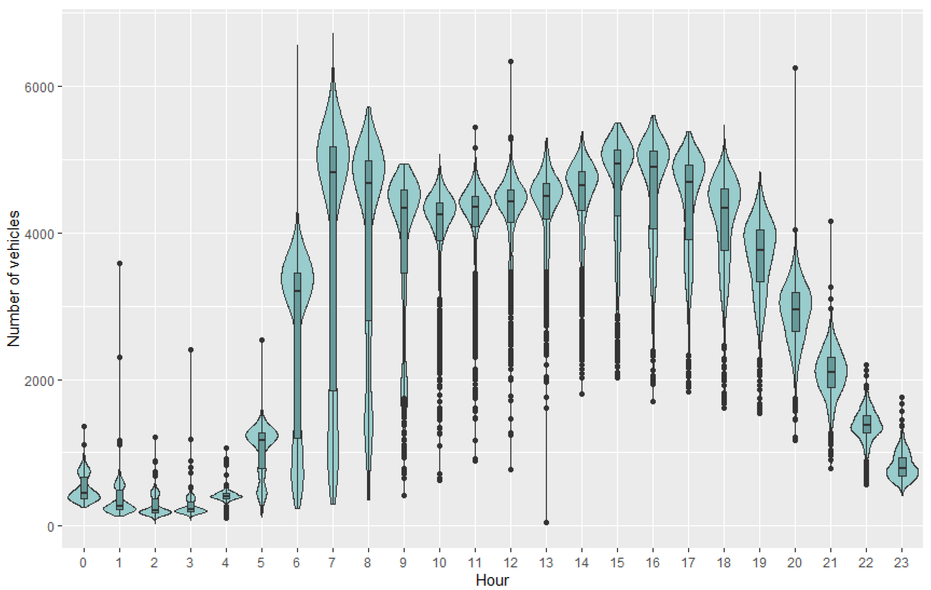
Traffic data were provided by the Traffic and Public Transport Management Department of the Roads and City Maintenance Board in Wrocław. The data contain counts of all vehicles (cars, buses, trucks, etc.) passing through the measurement intersection in a given traffic lane. The numbers of vehicles are recorded with a camera at 15-min intervals. In order to maintain equal time intervals for all factors, the values were aggregated into hourly counts. This operation reduced the noise while maintaining the characteristics of the original distribution. Out of the set of 26,304 cases, 212 gaps and 8 clear outliers resulting from failures of the measuring system were removed. Traffic flow is characterized by daily periodicity (Figure A1). There are two peaks: in the morning from 7:00 to 8:00 a.m., and in the afternoon between 3:00 and 5:00 p.m. The daily maximum of vehicles passing through the intersection during the three years under consideration was 6713 (

Table 1. Descriptive statistics for independent variables by season.

	Average					Minimum Value					Maximum Value
	All	Spr.	Sum.	Aut.	Win.	All	Spr.	Sum.	Aut.	Win.	All	Spr.	Sum.	Aut.	Win.
NO2	50.4	50.9	51.8	50.1	48.8	1.7	4.2	4.7	3.7	1.7	231.6	192.4	200.2	231.6	179.7
NOx	142.2	127.4	116.7	163.8	160.6	3.9	5.6	5.3	8.1	3.9	1728.0	1216.8	572.9	1728.0	1565.7
Traffic flow	2771	2803	2758	2855	2669	30	30	154	110	44	6713	5712	6713	5503	5599
Wind speed	3.1	3.1	2.6	3.1	3.7	0.0	0.0	0.0	0.0	0.0	19.0	16.0	19.0	16.0	15.0
Air temp.	10.7	10.1	19.9	10.4	2.3	−15.7	−4.6	7.2	−5.3	−15.7	37.7	31.0	37.7	34.8	15.4
Sunsh. dur.	0.23	0.27	0.36	0.16	0.10	0.00	0.00	0.00	0.00	0.00	1.00	1.00	1.00	1.00	1.00
Rel. hum.	74.9	70.7	67.6	80.0	81.0	20.0	21.0	20.0	25.0	30.0	100.0	99.0	99.0	100.0	99.0
Air press.	1003	1002	1002	1003	1004	960	980	978	969	960	1028	1021	1015	1022	1028
n	25,867	6396	6490	6508	6473

NO₂. NO_x—pollution concentration (µgm⁻³), traffic flow (veh), wind speed (ms⁻¹), air temperature (°C), sunshine duration (h), relative humidity (%), air pressure (hPa), n—number of valid observations.

). The annual average daily traffic at this intersection amounts to 65,470 vehicles.

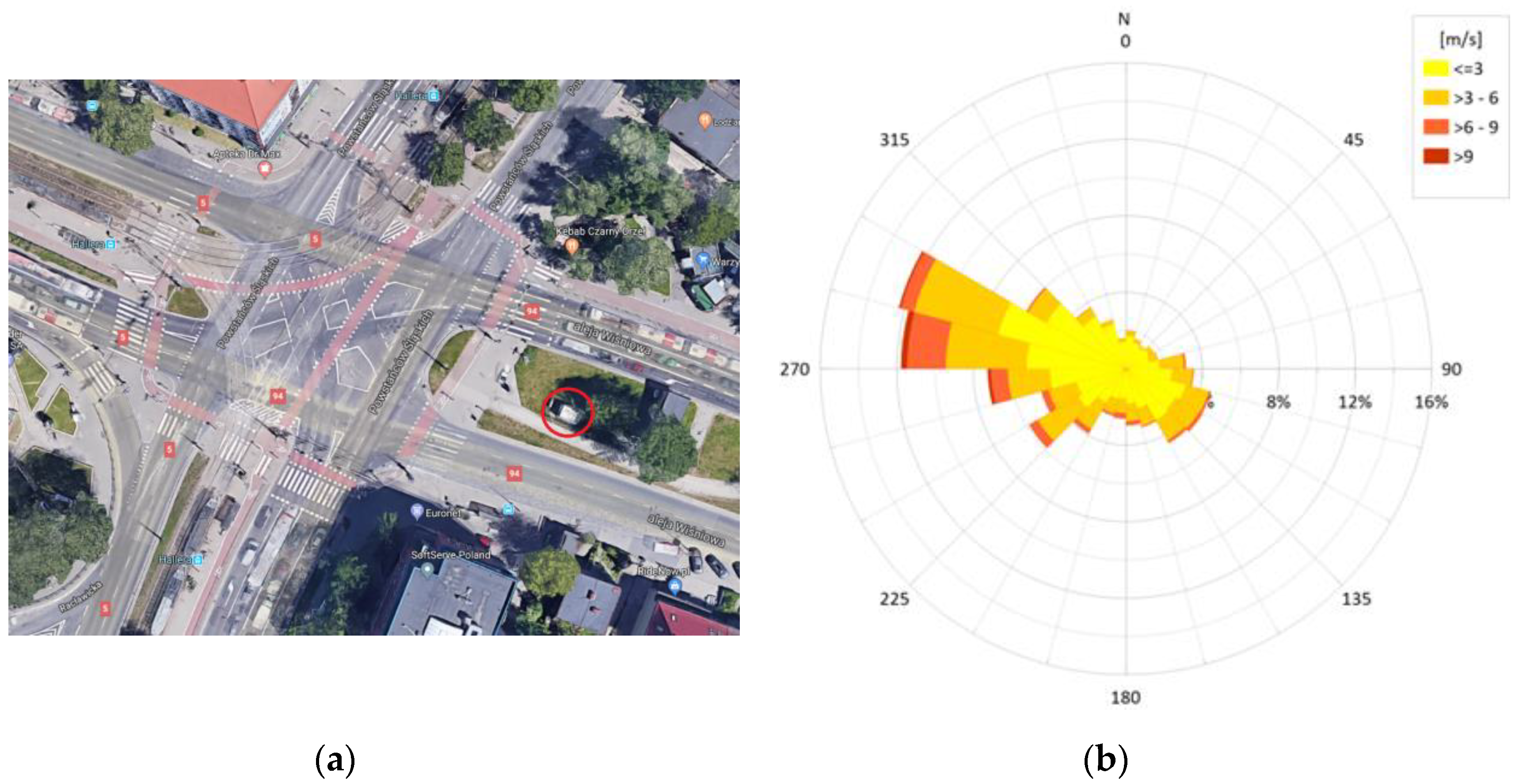
Meteorological hourly data were provided by the Institute of Meteorology and Water Management (IMGW) at only one station in Wrocław, located on the outskirts of the city 9 km from the intersection in a straight line (GPS coordinates: 51.1050N, 16.9000E; height 120 m a.s.l.). The meteorological data set contains air temperature, solar duration, wind speed, air pressure, and relative humidity. Clear seasonal variations in temperature can be observed which are characteristic of a transitional climate type subject to both oceanic and continental influences. The annual average air temperature in 2015–2017 in Wrocław was 10.7 °C (Table 1). The air temperature in the study period varied from slightly below −10 °C in winter to just over 30 °C. The average wind speed in Wrocław was 3.1 ms⁻¹ during the study period. The city did not experience very strong winds, as the maximum observed was 19 ms⁻¹ for one hour at 10 p.m. on 23 July 2017. Prevailing westerly and northwesterly winds accounted for about 50% of all winds.

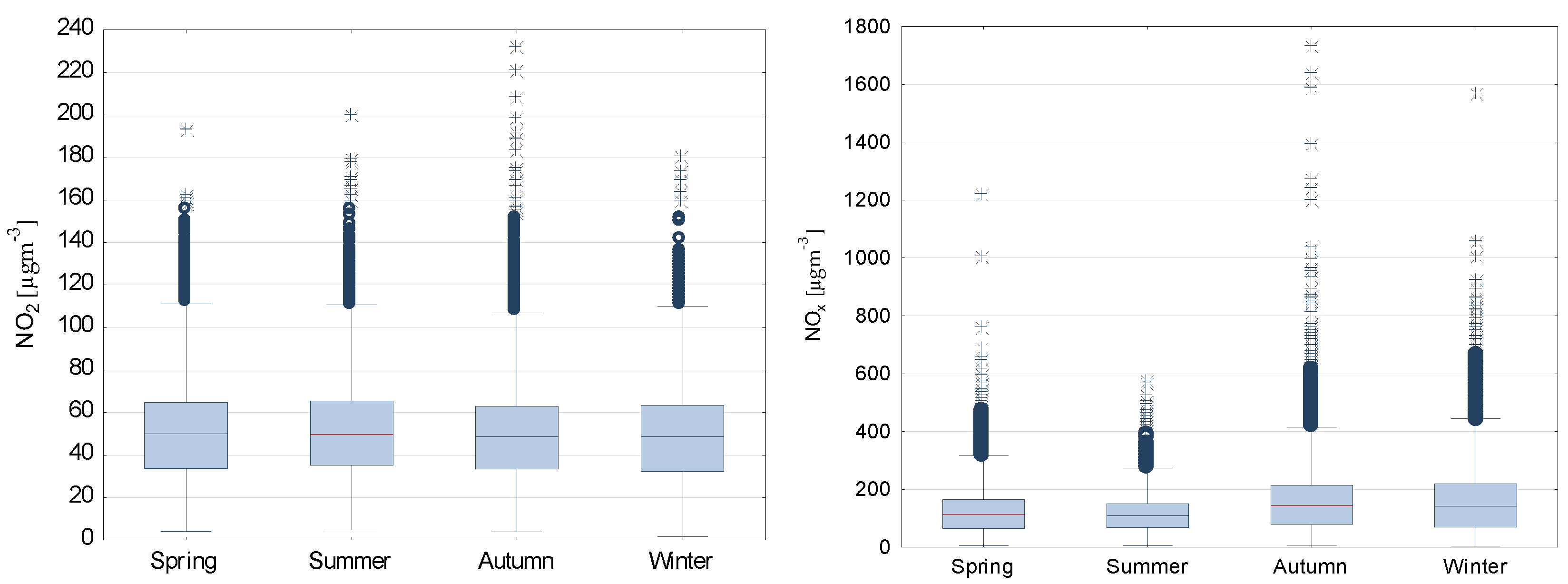
Air pollution data are collected by the Provincial Environment Protection Inspectorate and measured at hourly intervals. The measuring station (GPS coordinates: 51.0864N, 17.0127E; height 125 m a.s.l.) is located in the direct vicinity of the intersection with traffic measurement (30 m from the middle of the intersection). It can therefore be concluded that the distance between the pollutant measuring point and the source (intersection) does not play a significant role. There were 117 h (cases) of missing data during the study period, which were removed from the data set. The concentrations of NO₂ and NO_x reveal a clear daily (Figure A2) and seasonal (Figure 1) variation. The daily peaks roughly coincide with the peaks of traffic flow. The highest concentration variation occurs in autumn. This is particularly noticeable for NO_x. The nitrogen oxide concentrations in summer are the least differentiated, which means that the proportion and diversity of NO increases in summer. NO₂ concentration shows little annual seasonality, whereas NO_x compounds display significantly higher values in winter and autumn (hourly average: 160.6 and 163.8 µgm⁻³, respectively) than in summer (116.7 µgm⁻³). The maximum values of both of pollutants were reported in autumn (231.6 and 1728.0 µgm⁻³, respectively).

3. Methods

3.1. Multi-Objective Optimization

Given a data set $A$ with $n$ independent variables $A_1,\cdots A_n$ (in our case, traffic and meteorological data) and one observed variable $B$ (in our case, the concentration of a pollutant), solving a lag (linear) regression consists of solving the equation formulated as:

$$B\left(t\right) = c_0+{\displaystyle \sum }_{i=1}^n {\displaystyle \sum }_{l=0}^{p_i}{c}_{i,l}·A_i\left(t-l_{ }\right)+ϵ$$

(1)

In other words, we use the value of each independent variable $A_i$ not only at time $t$, but also at time $t-1,t-2,\cdots ,t- p_i$ to explain $B$ at time $t$; each $A_i\left(t-l\right)$ is associated to a coefficient $c_{i,l}$, which must be estimated, along with each $\mathrm{maximum} \mathrm{lag}$ $p_i$. Now, we work under the additional assumption that, for each $i$, there is precisely one lag $l_i$, such that $A_i\left(t-l_i\right)$ influences the output more than any other lag. Under such an assumption, the model that we are assuming becomes:

$$B\left(t\right) = c_0+{\displaystyle \sum }_{i=1}^n c_i·A_i\left(t-l_i\right)+ϵ$$

(2)

Moreover, in some contexts, a polynomial explanation model fits better than a linear one, yet preserving the possibility of an intuitive interpretation. From the mathematical point of view, the inverse problem that corresponds to searching for a polynomial model is a simple generalization of the previous equation:

$$B\left(t\right) = c_0+{\displaystyle \sum }_{i=1}^n c_i·A_i{(t-l_i)}^{e_i}+ϵ$$

(3)

so that our ultimate purpose is to find the optimal coefficient $c_i$s, the optimal lags $l_i$s, and the optimal exponents $e_i$s, for each predictor. We work out this problem as an optimization problem.

A multi-objective optimization problem (MO) can be formally defined as the optimization problem of simultaneously minimizing (or maximizing) a set of k arbitrary functions:

$$\{\begin{array}{c}min/\max f_1\left(\overline{x}\right)\\ min/\max f_2\left(\overline{x}\right)\\ \begin{array}{c}\dots \\ min/\max f_k\left(\overline{x}\right)\end{array}\end{array}$$

(4)

where $\overline{x}$is a vector of decision variables. Considering a multi-variate time series $A_1\left(t\right),\cdots ,A_n\left(t\right),B\left(t\right)$ with $m$ distinct observations, let $\overline{x} = \left(x_1,\cdots ,x_n\right)$be a vector of decision variables with domain $\left[-1,\cdots ,m\right]\subset \mathbb{N}$. Let $M$ be the maximum of $\overline{x}$ (called $\mathrm{maximum} \mathrm{lag}$ of $\overline{x}$). The vector $\overline{x}$ entails a lag transformation of the original data set into a new data set with $m-M$ observations, in which the feature (time series) $A_i$ is lagged (i.e., delayed) by the amount $\overline{x}\left(i\right)$. The particular case of a variable $\overline{x}\left(i\right)=-1$is interpreted as excluding the column $A_i$ from the problem (entailing an implicit feature selection method). Similarly, let$\overline{y} = \left(y_1,\cdots ,y_n\right)$a second vector of decision variables with domain ${\mathbb{N}}^{+},$ for each variable $A_i$, we interpret $\overline{y}\left(i\right)$ as the exponent to which $A\left(i\right)$ is raised. So, in conjunction, the pair $\overline{x}$, $\overline{y}$ entails a transformation of the initial data set into a new data set with $m-M$ observations, in which the feature (time series) $A_i$ is lagged (i.e., delayed) by the amount $\overline{x}\left(i\right)$, and raised to the power of $\overline{y}\left(i\right)$.

After applying a transformation, the resulting data set can be passed to any linear regression algorithm $ℒ$to solve the inverse problem associated with it. Now, in order to evaluate a candidate solution, let us consider the following function:

$$CARD\left(\overline{x}\right) = {\displaystyle \sum }_{i=1}^n\{\begin{array}{c} 0 if x_i\ne -1\\ 1 otherwise\end{array}$$

(5)

by means of which we count the number of selected features that play a role in the model, and

$$MAXEXP\left(\overline{y}\right) =\underset{1\le i\le n}{\max }\left\{\overline{y}\right\}$$

(6)

by means of which we measure the maximum exponent of the polynomial equation. Let:

$$ℱ\left(\overline{x},\overline{y}\right)$$

(7)

be any function that measures the performances (for example, the correlation coefficient) of $ℒ$ in estimating the parameters of the linear function that uses: (i) the features chosen by $\overline{x}$only, and (ii) raised to the power indicated by $\overline{y}$. Then, a multi-objective optimization model can be obtained by instantiating the generic formulation of an optimization problem as:

$$\{\begin{array}{c}min/max ℱ\left(\overline{x},\overline{y}\right)\\ min CARD\left(\overline{x}\right) \\ min MAXEXP\left(\overline{y}\right)\end{array}$$

(8)

3.2. Implementation, Algorithms, and Strategy

Multi-objective evolutionary algorithms are known to be particularly suitable for performing multi-objective optimization, as they search for multiple optimal solutions in parallel. In this experiment we chose the NSGA-II algorithm (Non-dominated Sorted Genetic Algorithm), which is available open-source from the suite jMetal [33]. NGSA-II is an elitist Pareto-based multi-objective evolutionary algorithm that employs a strategy with a binary tournament selection and a rank-crowding better function, where the rank of an individual in a population is the non-domination level of the individual in the whole population. As a black-box linear regression algorithm, we used the class linearRegression from the open-source learning suite Weka, run in 10-fold cross-validation mode with standard parameters and no embedded feature selected.

The overall strategy is as follows: first, we partitioned our data into training (30%) and test (70%), respecting the temporal ordering. We performed 10 independent executions using linear regression as a black box. Then, we chose the best-performing (and explainable) solutions and applied the corresponding transformation to the test data set. Finally, we learned a Random Forest model (from the learning suite Weka) on the resulting data set. Random Forest (RF) is a learning schema based on a set of simple decision trees. Each component tree is created for a randomly selected subset of data (sampling with replacement) and a subset of independent variables (predictors). In this analysis, each training set included another subset of 50% cases (sampling with return). The decision trees were built on four out of six predictors, randomly selected for each tree. The result of the random forest is taken by aggregating and averaging the individual predictions of each component tree. The C&RT method (Classification and Regression Trees) used to create random trees allows the validity of a variable to be determined based on an analysis of the frequency of the variable as a partition variable, taking into account the reduction of heterogeneity resulting from the division. The most important variable is assigned an importance of 100 and the other variables are then valuated proportionally, so feature importance is unitless [34]. As far as hyperparameters are concerned, we used 100 trees, no maximum depth, two samples as the minimum split, and one sample as the minimum leaf. The remaining ones cannot be defined in our chosen suite. Weka’s RF algorithm evaluates performances with the standard out-of-the-box methodology.

4. Results and Discussion

4.1. Lag Determination

Using multi-objective optimization, we determined the function that described the dependence of NO₂ and NO_x concentrations on meteorological factors and traffic flow. We assumed a maximum allowable power of the variable to be 3. As part of the process, we determined the delay (lag), the regression coefficient, and the power of each variable to maximize the fit of the model to real data. One should remember that the power of the variable was designated as the lowest possible one guaranteeing the best fit. In other words, the algorithm allowed a higher power than the first one, but the simplest (for interpretation) form of the function was preferred. Based on a 10-fold cross-validation process and on the selection of the most appropriate interpretation (in terms of the phenomena that occur in the atmosphere), we obtained linear functions with the delays presented in

Table 2. Delays (h) of the variable received through the multi-objective optimization process.

	Traffic Flow	Wind Speed	Air Temp.	Sunshine Duration	Relative Humidity	Air Pressure
NO2	1	3	0	2	7	0
NOx	1	2	0	10	0	0

. The fact that a linear function was obtained proves that the relationship is indeed linear and not of a higher degree.

For both NO₂ and NO_x, traffic flow from one hour prior has the largest influence on current concentration. This is the time that elapses from the emission of pollutants in the vicinity of the intersection until the pollution cloud reaches the sensor which measures the concentration of nitrogen oxides. The lower the wind speed is, the longer this time is. It should be remembered that the time for analysis purposes is rounded off to one hour. Therefore, a delay of 31 min and a delay of 1 h and 29 min will be both identified in the model as a delay of 1 h.

Wind speed has an impact on the evacuation of pollution. The stronger the wind speed, the more intense the evacuation and the lower the pollution concentration. Due to the distance of 9 km between the intersection and the meteorological station, the effect of wind speed is delayed by 2–3 h. This is a consequence of the time needed for the air masses to reach the air quality measurement station. In Wrocław, westerly and northwesterly winds prevail, i.e., blowing from the meteorological station to the city center (Figure A3). At an average wind speed of 3.1 ms⁻¹ covering a distance of 9 km, taking into account the roughness of urban buildings, takes from two to three hours. Delays are determined with an accuracy of one hour so the difference in values may be due to rounding. The actual air temperature is positively correlated with the current NO₂ and NO_x concentrations. In other words, high concentrations of pollutants occur at higher temperatures, and vice versa—low concentrations occur at lower temperatures. In addition, during the day—when the temperature is higher—the concentrations of pollutants are also higher. The occurrence of increased NO₂ concentrations at higher temperatures may be due to thermal decomposition of peroxyacetyl nitrates transported from other regions [35,36]. However, at night—when emissions and the temperature are lower—the NO₂ concentrations are lower. This state is the result of many processes and chemical reactions taking place at night; for example, chemical reactions transforming NO₂ into N₂O₅ or, conversely, NO oxidation with ozone to form NO₂.

Sunshine duration has a very important influence on chemical reactions with nitrogen oxides. Under the influence of sunlight, the Leighton relationship occurs [37]. NO₂ disintegrates into NO and ozone. At the same time, the reverse reaction occurs. During daylight hours, NO, NO₂, and O₃ concentrations persist in the photostationary state. The time to reach a stationary state depends on the NO₂ concentration and ranges from several minutes to tens of minutes [38]. This phenomenon is confirmed by the received impact of the two-hour delay in sunshine duration. The impact of the seven-hour delay in relative humidity on NO₂ concentration may result from a large inertia of humidity terms of the change in cloud cover. Air pressure is another meteorological condition that indirectly influences pollution concentration through the relationship with the type of cloud cover and precipitation (atmospheric fronts). With respect to air pressure, the value with the highest impact on nitrogen oxide concentration is the current one.

NO_x is the sum of NO and NO₂ concentrations. Consequently, the transformation of nitric oxide into nitrogen dioxide and vice versa does not change the NO_x concentration. Unlike NO₂, sunshine duration has the strongest impact on NO_x with a ten-hour delay—the opposite part of the day. Thus, the night after a sunny day, a relatively high NO_x concentration can be observed. The current relative humidity influences the current NO_x concentration (delay equals 0). High humidity from cloud cover and or precipitation prevents the chemical reactions between NO_x and volatile organic compounds (VOC) from occurring. Thus, nitrogen oxides float in the air, increasing the concentration.

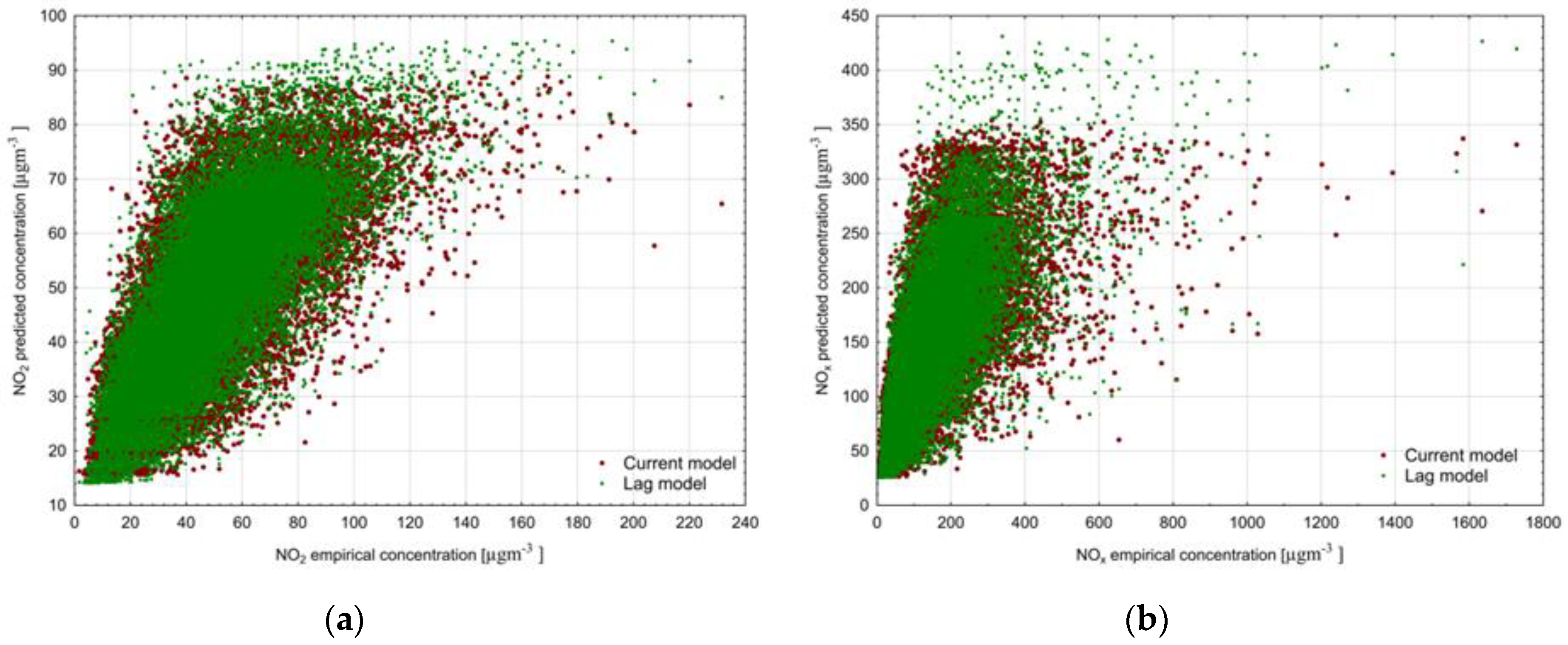
4.2. Random Forest Fitting

In the next step, we built two RF models: (1) using current values of predictors and (2) using lagged values (values of predictors with a delay) for each pollutant: NO₂ and NO_x. Then, we compared the impact of lag variables on the quality of model fit (

Table 3. Goodness of the measures.

	Equation
R2	${\mathrm{R}}^2=1-\frac{{{\displaystyle \sum }}_{i=1}^N{\left(y_i-{\widehat{y}}_i\right)}^2}{{{\displaystyle \sum }}_{i=1}^N{\left(y_i-\overline{y}\right)}^2}$
Mean Absolute Deviation Error	$\mathrm{MADE}=\frac{1}{N}{\displaystyle {\displaystyle \sum }_{i=1}^N}\left|{\widehat{y}}_i-y_i\right|$
Mean Absolute Percentage Error	$\mathrm{MAPE}=\frac{1}{N}{\displaystyle {\displaystyle \sum }_{i=1}^N}\frac{\left|{\widehat{y}}_i-y_i\right|}{\left|y_i\right|}$
Root Mean Square Error	$\mathrm{RMSE}=\sqrt{\frac{1}{N}{\displaystyle {\displaystyle \sum }_{i=1}^N}{\left({\widehat{y}}_i-y_i\right)}^2}$

) and assessed the impact (importance) of each of the factors in both models on the predicted values of the concentration of pollutants. The comparison of model fit quality including only current predictor values broken down by season is presented in

Table 4. Goodness of fit coefficient for NO₂ modeling.

	Full dataset		Spring		Summer		Autumn		Winter
	Current	Lag	Current	Lag	Current	Lag	Current	Lag	Current	Lag
R2	0.51	0.56	0.51	0.55	0.48	0.48	0.52	0.59	0.54	0.62
MADE	12.2	11.6	12.3	12.0	13.1	13.1	12.0	11.1	11.3	10.2
MAPE	0.26	0.24	0.26	0.25	0.26	0.26	0.25	0.23	0.26	0.24
RMSE	16.2	15.4	16.3	15.5	17.0	16.9	16.6	15.3	14.9	13.6
r	0.72	0.75	0.72	0.75	0.70	0.70	0.72	0.78	0.74	0.79

r—Pearson correlation coefficient.

. For the entire 2015–2017 measurement period, the model containing lagged variables turned out to be better suited to the empirical data, as indicated by the values of all goodness of fit measures. Both models, current and lag, best describe the relationship between pollutant concentrations and meteorological factors and traffic flow for winters. For the winter period (December–February) the greatest improvement in model fit also came after taking into account lag variables, probably because in winter wind speeds are low and the concentration is more influenced by local traffic than by emissions in the surroundings. In addition, stagnation processes and atmospheric inversions also have a significant impact on the retention of pollutants. A slightly smaller improvement in the quality of fit occurred in the autumn. There was no change in the quality of fit for NO₂ modeling during the warmer part of the year (June–August). This was probably caused by the lack of some important factor determining the NO₂ concentration during periods of strong sunshine and high air temperature.

Due to the greater variation in NO_x values (coefficient of variation for NO₂ is 46%, and for NO_x 73%) it is more difficult to predict its values effectively. This is generally indicated by less goodness of fit than for NO₂ (

Table 5. Goodness of fit coefficient for NO_x modeling.

	Full Dataset		Spring		Summer		Autumn		Winter
	Current	Lag	Current	Lag	Current	Lag	Current	Lag	Current	Lag
R2	0.46	0.52	0.45	0.50	0.42	0.46	0.41	0.49	0.46	0.51
MADE	47.9	45.3	44.3	42.3	37.2	36.5	54.9	51.0	55.1	51.4
MAPE	0.35	0.33	0.34	0.32	0.31	0.30	0.38	0.35	0.38	0.36
RMSE	76.3	72.2	63.9	60.7	50.4	48.8	94.9	88.6	87.4	83.1
r	0.68	0.72	0.68	0.72	0.66	0.69	0.66	0.72	0.68	0.72

r—Pearson correlation coefficient.

). As in the case of nitrogen dioxide, for NO_x the greatest improvement in fit quality occurred in autumn and winter. It is worth noting that taking into account the delay of variables resulted in an improvement in the quality of NO_x model matching in the summer as well. This means that in a situation where the transformations of NO into NO₂ and vice versa are not relevant for the concentration of the pollutant (NO_x = NO + NO₂), determining the correct delay of the variable is an effective way to improve the model.

4.3. Random Forest Variable Importance

The method of determining the relationship between the concentration of pollution and environmental factors implemented in the paper was done to determine the impact of each of the factors. Therefore, feature importance values were used to assess the impact of the factor. In each model, current and lag, feature importance values for each predictor were determined (

Table 6. Feature importance of variables in Current and Lag models.

	NO2		NOx
	Current	Lag	Current	Lag
Traffic flow	100	100	100	100
Wind speed	46	43	49	59
Air temperature	26	22	39	40
Relative humidity	24	41	30	29
Sunshine duration	14	17	17	18
Air pressure	9	9	29	26

). An analysis was also made by season. The highest influence came from traffic flow, the only predictor related with the source of pollution (emission). Wind speed has about half as much of an influence on the concentration of nitrogen oxides in the air—the only factor among those studied which directly affects the evacuation of pollution. These findings are in accordance with analyses performed for other regions, e.g., [21] in Madrid or [8] in Oslo. Other factors (air temperature, relative humidity, sunshine duration, and air pressure) indirectly affect the final concentration value. Their impact is therefore significantly smaller.

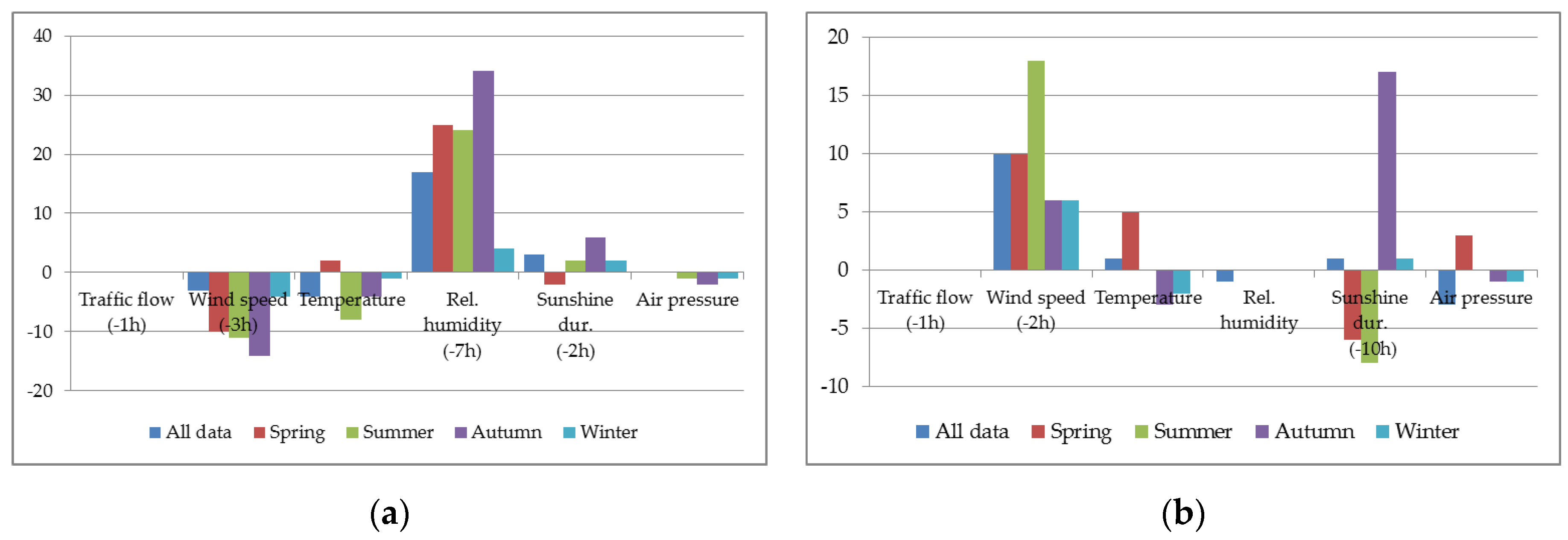
The change of feature importance as a result of taking into account variable delays is presented graphically in Figure 2. It can be seen that delays in the predictors for NO₂ and NO_x have different impacts on the importance of dependent variables. The bars represent the values of the relevant differences in feature importance between the current and lag models. Optimal lags changed the significance of variables in the NO₂ and NO_x models. Only traffic flow with a one-hour delay is still the most important factor determining the concentration of both pollutants.

When drawing conclusions about changes in the importance of variables, remember that feature importance values are related to the most important variable that has been assigned the value of 100 (here, it was always traffic flow). Therefore, a change in feature importance value can only be assessed as a change in relation to the significance of traffic flow. Factoring in a three-hour delay in wind speed reduced the significance of this variable in relation to traffic flow for emissions in NO₂ models. However, it cannot be unequivocally stated whether it was the load of pollutants with a one-hour delay that grew in importance, or whether the intensity of evacuation was less intense. Relative humidity increased significantly when it was introduced to the model with a delay of seven hours. This means that it is important in modeling to recognize the inertia of the response of individual meteorological factors to current weather conditions. An important role in NO₂ concentration modeling is played by the chemical reactions that occur in the atmosphere, which vary during the day due to sunlight and at night or on a cloudy day. Determining the optimal delay allows one to identify these relationships. The importance of air temperature, sunshine duration, and air pressure does not change after factoring in delays. Markedly different observations of the dependencies between feature importance in the lag modeling of NO_x do occur. The most visible changes were observed in the importance of wind speed. For each whole season—especially summer—wind speed became a more important variable. Therefore, correctly taking into account the lagged variables shows that in NO_x modeling wind speed is more important than what was suggested by the basic current model. An interesting phenomenon appeared for the importance of sunshine duration. When analyzing the entire research period, the impact of this variable in both models (current and lag) was the same in relation to traffic flow, even when separated by season. It turns out that this is the outcome of a significantly higher impact in autumn (about twice as important) than in spring and summer. It can be supposed that extremely high NO_x concentrations in the afternoon and evening in the autumn are related to the sunlight that day. A delay in relative humidity did not affect the importance change in relation to traffic flow.

Following the above argumentation, it can therefore be concluded that determining the optimal delays (lag variable) of environmental factors in the modeling of pollutant concentration significantly increases the accuracy of the model and is confirmed by the physicochemical developments on the atmosphere. The goodness of fit values of the presented models, as to orders of magnitude, are similar to those reported by other researchers. For example, for average monthly NO₂ concentration, Zhu et al. [17] obtained an RMSE of 11.0 µgm⁻³ and Zhan of 13.3 µgm⁻³ for daily NO₂ modelling in China; Kamińska and Turek [25] reported a daily average of 7.47 µgm⁻³ for modelling in Wrocław; for the Polish capital—Warsaw—Holnicki et al. [39] obtained a normalized mean square error of 0.070. The application of the optimal lag variable models presented herein enhanced the model fit, as measured by RMSE, from 16.2 µgm⁻³ to 15.4 µgm⁻³ for the entire three-year period and from 14.9 µgm⁻³ to 13.6 µgm⁻³ for winter. The R² of 0.56 (10% greater than without lag variables) for NO₂ confirms the effectiveness of the model and provides better accuracy than that presented by, for example, Laña [21] (${\mathrm{R}}^2=0.53$).

In full generality it can be concluded that determining the optimal delay for environmental variables and including such lag variables as predictors increases the accuracy of the model. The only exception is the summer season in the modeling of NO₂ concentration. Despite the changes identified in feature importance in comparison to the current model, the model fit did not increase. This is probably due to the lack of some other factors which significantly affect the concentration of NO₂ during periods of intense sunlight and high temperature; these may include rainfall, solar intensity, radiation, or concentrations of pollutants that react intensively with nitrogen oxides, such as ozone. However, such analysis delves into the details of atmospheric chemistry, which was not the purpose of this study. Further studies should consider extending the set of predictors with new variables.

The method for determining the optimal delay for each independent variable and input of this lag variable model is a very general method; it may be utilized in any air pollution model regardless of the factors and type of pollution under study. Conclusions regarding the linearity of each of the factors in this paper, however, are local and refer only to the conditions considered herein. Nevertheless, the general, most important goal is to obtain ideally the first power of all variables. The impact of climatic conditions (here, the seasons) can also be regarded as significant in full generality. The results suggest that in similar studies for other locations or pollutants, the seasonal variability of meteorological conditions should be considered, and that the impact of factors determining air pollution should be assessed with this variability taken into account.

The idea of determining the effect of delayed values (from a few hours prior) of the key factors on the concentration of pollution is very general. As a mathematical method, it can be applied to any pollution and any set of explanatory variables. The example of the specific intersection in Wrocław presented herein leads to locally valid conclusions. The specific characteristics of the wind direction distribution (here, winds parallel to the intersection’s axis in the direction of the air pollution sensor predominate) suggests using a delay in relation to the time of air mass movement and pollution clouds. The consequence of the significant distance between the intersection and the meteorological station, as well as the city-specific buildings (terrain roughness), is a delay in the variable wind speed. These observations confirm the effectiveness of the model and the correctness of factoring in delays in such modeling. For a different location, the delays would likely be different because they would result from the specific nature of that location. Nevertheless, the interpretation and their impact on the quality of the model are equally valuable.

4.4. Limitations

The presented methodology is subject to certain limitations. In a RF regression problem, the range of predictions values is bound by the highest and lowest labels in the training data. Due to the RF construction consisting in averaging the predicted values from all constructed random trees, this model does not work in predicting extremely high values (concentration peaks) when we do not take into account the past values of the dependent variable (Figure A4). Although the distance between the intersection and the meteorological station (9 km) was included in the lag model in the form of delays, which can be clearly seen in the example of wind speed the relationship between meteorological factors and air pollution concentration might be weakened by this long distance considering the footprint of sensors, especially when considering the heterogeneity of the urban fabric [40]. It should be remembered that each of the mathematical methods used (MO and RF) does not take into account physical and chemical phenomena occurring in the atmosphere in the process of creating/optimizing. Nevertheless, the obtained results (optimal delays and importance of variables) are consistent with the phenomena actually taking place in the atmosphere.

5. Conclusions

The paper presents an assessment of the impact of finding the optimal delay of an independent variable on a model of air pollution concentration (NO₂ and NO_x) in a street canyon. Based on the supposition that the current concentration of pollutants can be more strongly influenced not by current, but past factor values, we proposed a method for determining delays for this factors. We have developed a three-object optimization method to determine a polynomial function (with the power limited to three) that guarantees the best possible fit to the empirical data. For both NO₂ and NO_x compounds, the linear function proved to be the most appropriate. For both pollutants, a one-hour delay for traffic flow and a two- or three-hour delay for wind speed had a larger impact than the current values. Likewise, past sunshine duration values had a greater impact on current pollutant concentration values. For NO₂, this delay is two hours due to NO–NO₂ transformations. For NO_x, the delay is 10 h, which indicates that sunshine has a significant effect on nighttime concentration values. The delays determined by this analysis were used in a random forest model. The designated lag variables were taken as predictors. We developed four random forests: current models, using just the current values of the predictors, and lag models, using lagged variables, for NO₂ and NO_x separately. Considering individual seasons, the greatest changes in the importance of the delayed variables in NO₂ forecasting occurred in autumn. Wind speed from 3 h ago turned out to be a relatively less important variable in the lag model than the actual wind speed in the current model. Relative humidity from before 7 h in the lag model has gained the most in importance. In forecasting NO_x concentrations in autumn, the greatest increase in importance in the lag model compared to the current model occurred for the sunshine duration 10 h ago. In summer, the greatest increase in the impact of wind speed from 2 h ago was observed, compared to the actual values in the current model.

Taking into account factors in the form of lag variables also influenced the importance of variables, i.e., their impact on the level of pollution. For NO₂, the wind speed delay decreased its importance and relative humidity increased its importance in relation to traffic flow. For NO_x, a three-hour wind speed delay increased its importance in relation to traffic flow. Generally speaking, the method is universal. Detailed conclusions depend on local meteorological, topographical, and traffic conditions.