Article

Spatial and Temporal Exposure Assessment to PM2.5 in a Community Using Sensor-Based Air Monitoring Instruments and Dynamic Population Distributions

1
Department of Occupation Health, Daegu Catholic University, Gyeongbuk 38430, Korea
2
Center of Environmental Health Monitoring, Daegu Catholic University, Gyeongbuk 38430, Korea
3
Department of IoT Solution Biz, SK planet, Seongnam 13487, Korea
4
Department of Climate Change Action, Korea Testing & Research Institute, Gwacheon 13810, Korea
5
Department of Environmental Big Data, CHEMI. I. NET, Ltd., Seoul 07964, Korea
6
Department of Health, Environmental and safety, College of Health Industry, Eulji University, Seongnam 13135, Korea
7
Institute of Risk Assessment, Department of Chemical and Biological Engineering, Seokyong University, Seoul 02713, Korea
*
Author to whom correspondence should be addressed.
Atmosphere 2020, 11(12), 1284; https://doi.org/10.3390/atmos11121284
Submission received: 15 November 2020 / Revised: 25 November 2020 / Accepted: 26 November 2020 / Published: 28 November 2020
(This article belongs to the Special Issue Challenges in Measuring and Assessing Environmental Health)

Abstract

:
This research was to conduct a pilot study for two consecutive days in order to assess fine particulate matter (PM2.5) exposure of an entire population in a community. We aimed to construct a surveillance system by analyzing the observed spatio-temporal variation of exposure. Guro-gu in Seoul, South Korea, was divided into 2,204 scale grids of 100 m each. Hourly exposure concentrations of PM2.5 were modeled by the inverse distance weighted method, using 24 sensor-based air monitoring instruments and the indoor-to-outdoor concentration ratio. Population distribution was assessed using mobile phone network data and indoor residential rates, according to sex and age over time. Exposure concentration, population distribution, and population exposure were visualized to present spatio-temporal variation. The PM2.5 exposure of the entire population of Guro-gu was calculated by population-weighted average exposure concentration. The average concentration of outdoor PM2.5 was 42.1 µg/m3, which was lower than the value of the beta attenuation monitor measured by fixed monitoring station. Indoor concentration was estimated using an indoor-to-outdoor PM2.5 concentration ratio of 0.747. The population-weighted average exposure concentration of PM2.5 was 32.4 µg/m3. Thirty-one percent of the population exceeded the Korean Atmospheric Environmental Standard for PM2.5 over a 24 h average period. The results of this study can be used in a long-term aggregate and cumulative PM2.5 exposure assessment, and as a basis for policy decisions on public health management among policymakers and stakeholders.

1. Introduction

Fine particulate matter (PM2.5) is an air pollutant that is classified as a Group 1 carcinogen by the International Agency for Research on Cancer [1]. It can cause various adverse health effects. The World Health Organization suggested that a 10 µg/m3 increased concentration of PM2.5 was associated with a 6–13% increase in long-term exposure risk of cardiopulmonary disease mortality rate [2]. Also, Di et al. accounts for a 7.3% increase in all-cause mortality [3]. A PM2.5 exposure assessment in a community such as an industrial complex is crucial in terms of public health since it can provide the data required to develop a suitable management plan [4].
The necessity of an exposure surveillance system is emerging in the field of exposure science. An exposure or health surveillance system can be defined as a monitoring system that tracks aggregate and cumulative exposure of the human body to the hazardous agent, and enables assessment of the population exposure, considering the spatial and temporal variation of air pollutants (e.g., emission source, reaction, and deposition) and the population’s time-activity pattern [5,6,7,8]. Although the Korean Ministry of Environment provides information for PM2.5 measured by beta attenuation monitor (BAM), these data cannot reflect the actual exposure of the population [9,10]. An exposure surveillance system could be constructed with a sustainably gathered information about exposure concentration and population dynamics. Most recently, exposure assessments using low-cost sensors and mobile phone data have been performed [11,12,13].
When assessing population exposure, if the study area is divided into high-resolution grids and the results are summed, a reliable exposure assessment can be performed. To assess population exposure, it is necessary to gather information about the distribution of exposure concentration and population to incorporate the exposure concentrations and time-activity pattern. Many studies have suggested the relationship between PM2.5 concentrations and public health by analyzing long-term PM2.5 concentrations [14,15,16]. However, they mainly focused on outdoor exposure concentrations and only used data from the fixed-air monitoring stations. Since people spent most of their time indoors, indoor air quality should also be considered when assessing exposure to air pollutants. Zhang et al. assessed population exposure with relation to human cumulative exposure, using interpolation and population distribution based on census data [17]. There are limitations to assessing population exposure using the population distribution based on census data, because they were constructed with low resolution. Another technique is with the use of mobile phones to estimate population distribution [18]. The exposure of the entire population in a community can be estimated by population-weighted average exposure concentration (PWAC) [19]. PWAC is a method performed by weighting the rate of the number of people in a unit area—divided by the grid—per entire area to the exposure concentration in the unit area. By summing up all of PWAC, it is possible to assess the exposure of the entire population.
In this study, a pilot test was conducted to assess the population exposure of a community using the concentration of PM2.5 measured by sensor-based air monitoring instrument (SAMI) and the population distribution using mobile phone data.

2. Methods

2.1. Subject Area

The research was conducted on 1 and 2 October 2019 for 48 h in Guro-gu. Guro-gu is one of the 25 districts of Seoul, which is the capital city of Republic of Korea. It had a population of 435,560 in 2019, accounting for 4.5% of the population of Seoul, with an area of 20.12 km2. We divided this study area by 2204 grids of 100 m square (Figure 1).

2.2. Indoor and Outdoor Exposure Model

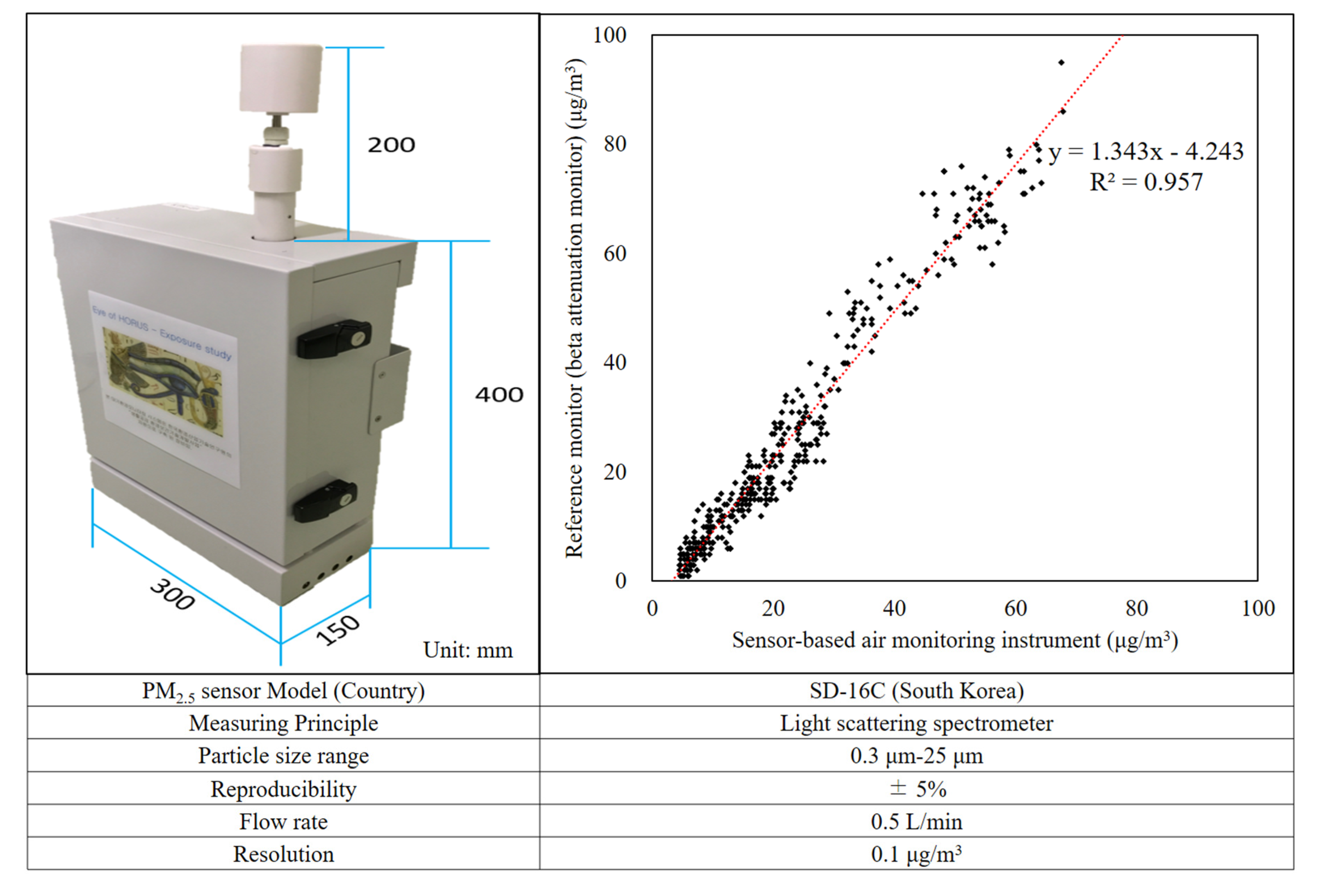
We installed 24 SAMIs with approximately 1 km2 scale resolution in Guro-gu. The SAMIs used in this study consisted of a set of sensors that can measure PM2.5 concentration, temperature, and relative humidity. The model used was designed to maintain a temperature of 20–30 °C and relative humidity of less than 70%, with a pretreatment control device and an integrated system. The detailed specification of the SAMI is shown in Figure 2. The PM2.5 concentrations measured by the SAMIs were collected every minute and transmitted to the G-Cloud (Government Cloud), which is a cloud computing service developed for the Korean government’s public institution launched in 2012 [20].
The outdoor PM2.5 concentrations of each grid were modeled by inverse distance weighting (IDW) method using SAMIs (Equation (1)):
z p = i = 1 n z i w i i = 1 n w i
where zp is the estimated concentration at site p, zi is the measured concentration at site i, wi is the weight of interpolation, and n is the number of SAMI used for interpolation
To estimate indoor PM2.5 concentration, we applied an indoor-to-outdoor (I/O) PM2.5 concentration ratio [21]. The I/O ratio of Guro-gu’s indoor buildings when adapted was 0.747, which is a result of simulating standardized the time–activity patterns of the general households in Seoul [22,23].

2.3. Population Distribution

Population distribution of Guro-gu was determined by the number of people in each grid estimated by a pilot pattern cell database (pCell DB). The pCell method uses one of the tracking locations of mobile phone user when the device cannot receive a GPS signal. It uses the positioning solution of the pattern matching method. The program had patterned station coordinates of the propagation environment of the service area in the database, and so determined the location of mobile phone users by matching the propagation characteristics with database. The pCell data from wireless communication systems identified the number of people without personal information except age and sex within a grid (100 m × 100 m), defined based on the coverage of signals from the base stations. The pCell data were the results that mobile network operators have been observing from each wireless tower signal coverage periodically. The size of each pCell population per each hour was estimated by mapping the coverage of whole wireless tower and mobile phone reports, which include the connecting tower identifications (IDs). Moreover, the pCell data used an algorithm approved by Korean National Statistical Office for converting mobile network operator population to whole community population. The estimated population distribution was averaged by the number of people in a grid for one hour, and sorted by dividing the population into five years of sex and age.
To estimate the population distribution in indoors and outdoors, we used time-activity analysis results that surveyed subjects under age 10 [24]. The subjects of the survey were selected across the nation using a stratified sampling method according to square root proportional allotment. It targeted 922 subjects by season (spring, summer, fall, and winter) from 2013 to 2014. The survey was conducted for two consequence days. The subjects were required to record their behavior and whether their locations were indoors or outdoors in the time-activity diary. In the case of the subjects who were too young to record their diary, the subjects’ parents recorded the results.
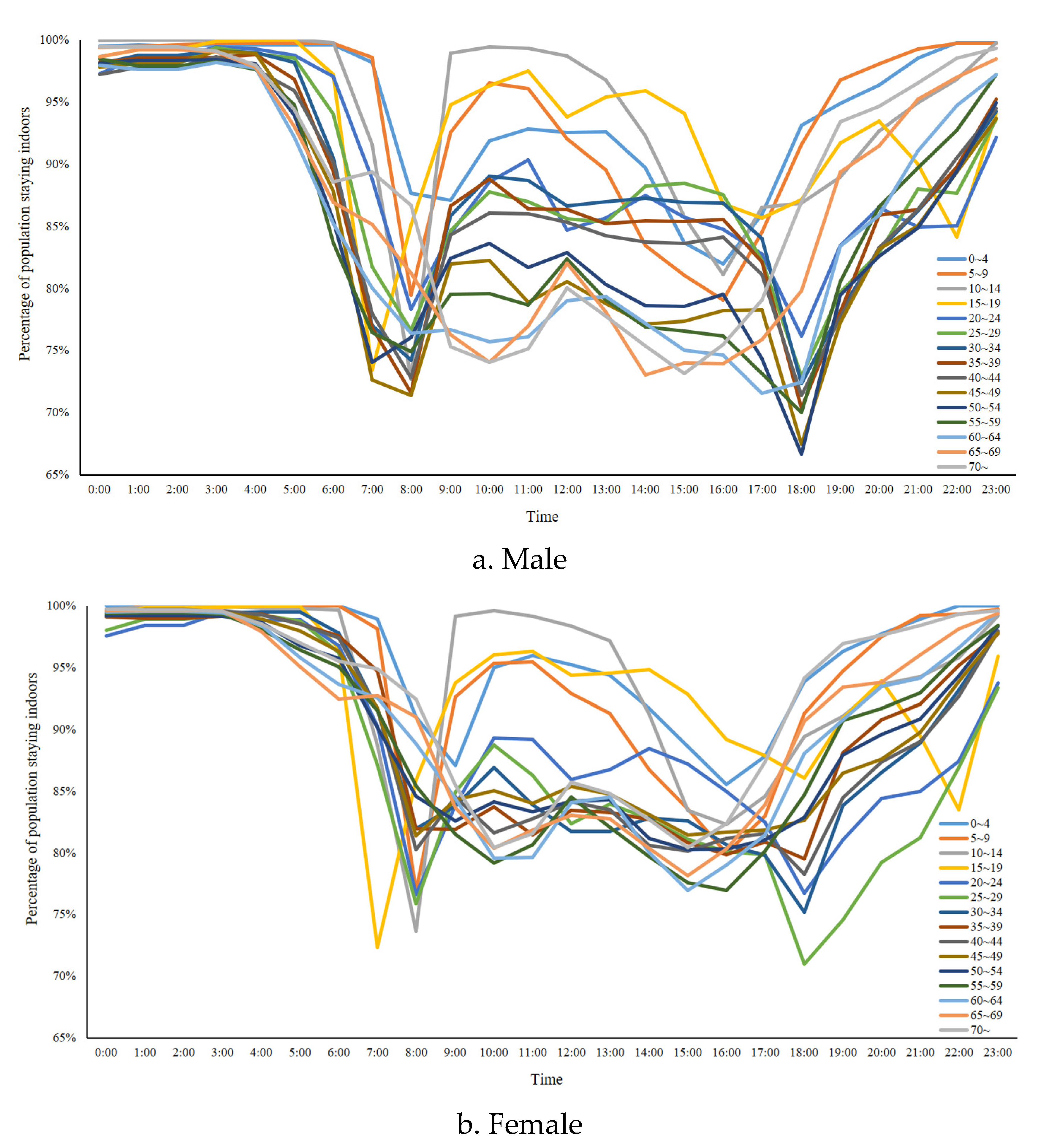
In the case of subjects age 10 or older, we used a Time-Use Survey dataset of 3,984 residents of Seoul. These data were published in 2016, and were downloaded from the Korean National Statistical Office’s website (http://kostat.go.kr/portal/korea/kor_nw/1/6/4/index.board). The Time-Use Survey is a national standardized survey that is conducted every five years. It records the behavior and location of the subjects in a time-activity diary. Participants were recruited across the country using a stratified sampling method according to a square root proportional allotment considering sex and age. The indoor microenvironments of the subjects were categorized into eight microenvironments: home, workplace, school, another house, bar or restaurant, other indoor places, places for walking (outdoors), and transport. For the Time-Use Survey data, the times spent in each microenvironment were not classified as either indoor or outdoor environments. Therefore, the indoor staying rate of each microenvironment presented in the Korean Exposure Factor Handbook was applied to the time spent in each microenvironment [25]. Table 1 presents the indoor staying rates according to the microenvironments. We applied these data together with that from Time-Use Survey to show the total indoor staying rates according to age, sex, and time. The trend is shown in Figure 3. We calculated the number of people indoors and outdoors from each grid by applying the staying rate of Figure 3 to the population distribution data.

2.4. Population Exposure

We assessed the population exposure using PM2.5 concentrations and the population distribution of each grid. The assessment of exposure was performed using the equation below (Equation (2)). To map the outdoor PM2.5 concentration, population distribution, and population exposure, we used Quantum GIS software version 3.16.
Population Exposure = cipi + copo
where ci is the indoor exposure concentration, co is the outdoor exposure concentration, pi is the number of people indoors, and po is the number of people outdoors.
To assess the exposure to PM2.5 of the entire population of Guro-gu, we calculated the PWAC by weighting the number of people to the exposure concentration in each grid (Equation (3)). To assess population exposure to PM2.5 probabilistically, we calculated the rate with the use of frequency analysis and histogram. The resulting rate of exposure exceeded the Korean Atmospheric Environmental Standard. We excluded the grid with a PWAC of zero (resulted from zero population) in the frequency analysis.
PWAC   =   i = i n c i p i + c o p o p i p o
where, PWAC is the population weighted average concentration (µg/m3), n is the number of the grid, ci is the indoor exposure concentration in grid n, co is the outdoor exposure concentration in grid n, pi is the number of people indoors in grid n, po is the number of people outdoors in grid n.

3. Results

3.1. Indoor and Outdoor Exposure Model

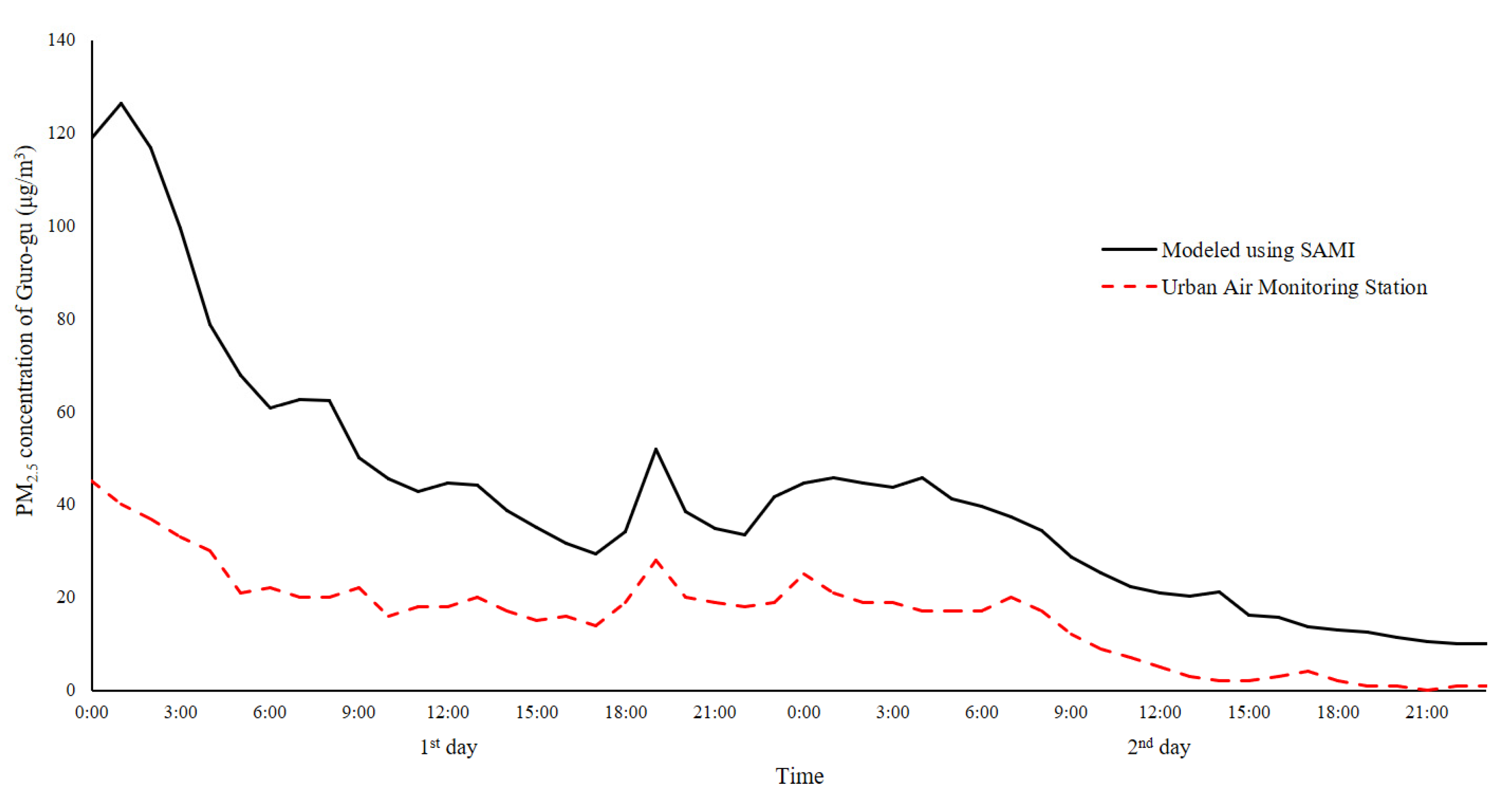
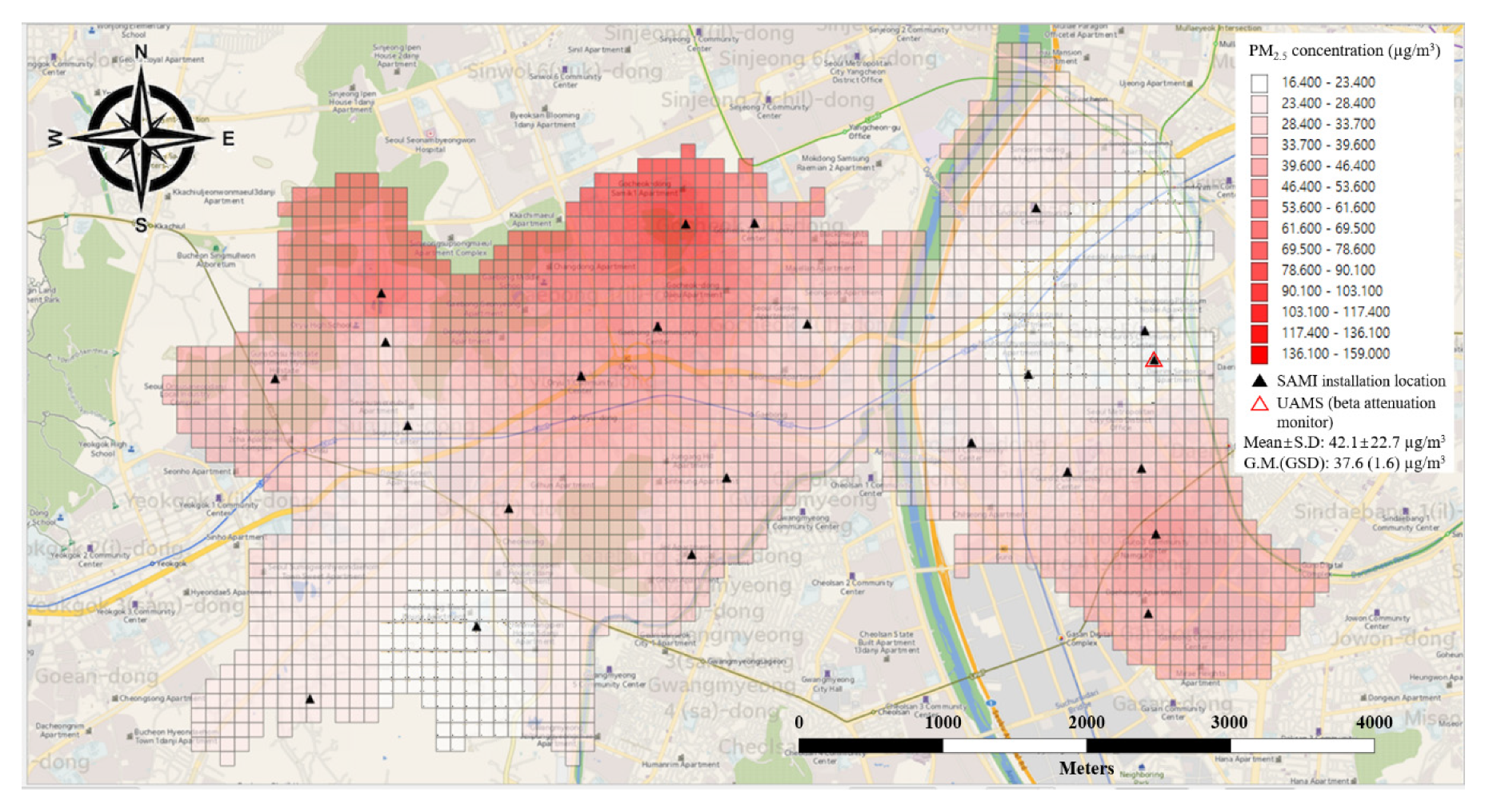
The temporal and spatial variations of the outdoor concentration of PM2.5 for 2 days are presented in Figure 4 and Figure 5. These variations in concentration are further illustrated as an animation in Figure S1. The temporal variation presented the entire average outdoor concentration in Guro-gu, modeled by SAMI and measured by an urban air monitoring station (UAMS) using the beta attenuation monitor. The average outdoor PM2.5 concentration in Guro-gu for 2 days was 42.1 µg/m3, and the standard deviation according to time and location was 27.7 µg/m3 and 22.7 µg/m3, respectively. The average concentration of UAMS for 2 days was 16.4 ± 10.5 µg/m3. The correlation between the modeled outdoor average concentration of the entire Guro-gu and UAMS is presented in Figure 6. The correlation coefficient (R2) was 0.8604, the slope was 0.3565, and the intercept was 1.0806.

3.2. Population Distribution

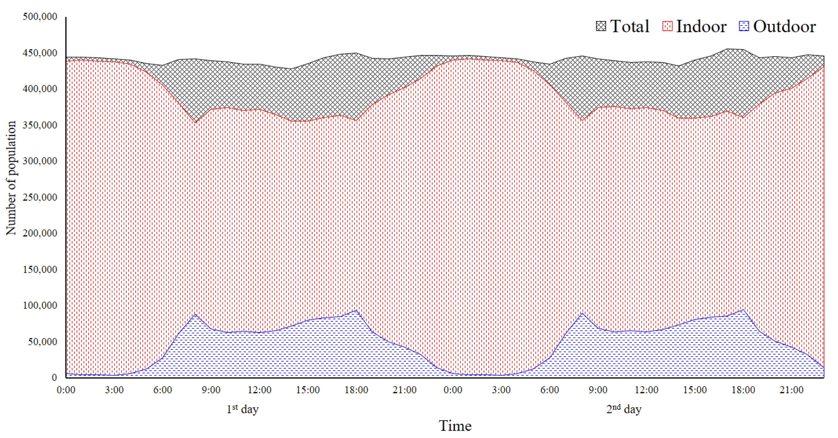
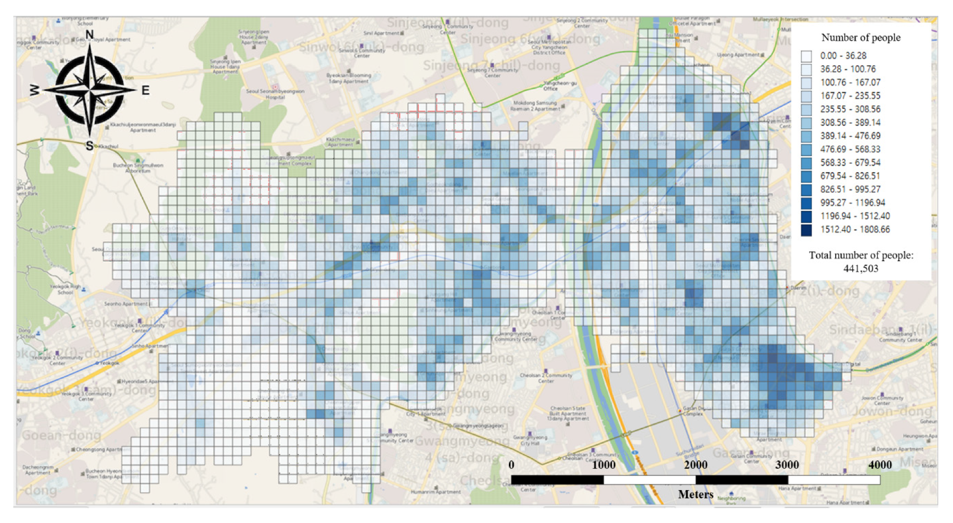
The temporal and spatial variations of the population in Guro-gu are presented in Figure 7 and Figure 8. For further illustration of the spatial and temporal variations of the total number of people in Guro-gu, we provided an animation as Figure S2.

3.3. Population Exposure

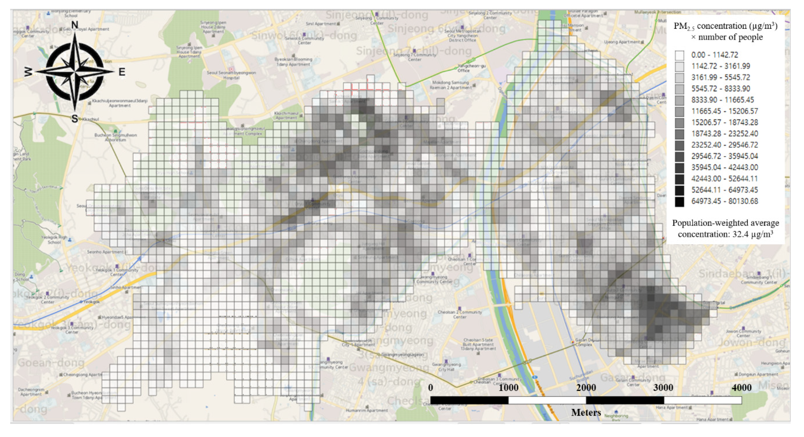
Figure 9 presents the population exposure to PM2.5 of Guro-gu. The PWAC of the entire population was 32.4 µg/m3. Also, an animation showing the spatial and temporal variations is presented in Figure S3.
The histogram of the PM2.5 PWAC is shown in Figure 10. Aout 97.5% and 31.4% of the studied population exceeded the Korean Atmospheric Environmental Standard for PM2.5 for both annual (35 µg/m3) and 24 h (15 µg/m3) averages, respectively.

4. Discussion

The PM2.5 exposure of the entire population was assessed by constructing an exposure surveillance system considering spatio-temporal variations. The exposure assessment for the entire population was reliable because the concentration of PM2.5 was modeled by a sensor-based air monitoring instrument that captures real-time measurements, data communication, and population distribution representing population dynamics. It was obtained by using a mobile phone. There were limitations in estimating indoor concentration and the distribution of the population indoors and outdoors. For instance, the I/O ratio was applied to estimate indoor PM2.5 concentrations, while the indoor staying rates according to age and sex were applied to indoor and outdoor population distributions. However, these could be representatives because the I/O ratio was a result of simulated standardized time-activity patterns of general Korean households, and the indoor staying rates by time were assessed based on demographical characteristics.
The PM2.5 concentration of Guro-gu was modeled using the IDW method and I/O ratio based on measurements by SAMIs. The modeled outdoor average concentration of PM2.5 in the entire Guro-gu was relatively lower than the one measured by the UAMS. It was determined that the concentration of PM2.5 near the UAMS was relatively low, as shown in the spatial variation (Figure 5). The UAMS that offers a representative concentration of PM2.5 of the local area has limitations to detect spatial variation, such as local air pollutant sources [26,27]. Recently, exposure assessment studies have widely been performed using low-cost sensors [28,29,30]. This methodology enables exposure assessment to air pollutants with relatively low cost and high resolution, and eases data management by using information and communication technology like wireless fidelity (WiFi) and long-term evolution (LTE) networks [31,32,33,34]. The IDW model used in this study to estimate PM2.5 concentration is one of the geostatistical models, which is more suitable for this study, in which multiple measurement spots are distributed, than the source-based model [35]. Recently, the methodologies using machine learning or deep learning technology to estimate ambient air pollutant concentrations have been widely used [36]. According to Yang et al., artificial intelligence technology and statistical models have been used as exposure models of air pollutants, and statistical models have shown relatively high accuracy until now [37].
The average I/O ratio of PM2.5 concentrations in apartment houses was applied to estimate indoor PM2.5 concentration. The I/O ratio in other microenvironments could be different [38]. However, the I/O ratio in this study and the previous findings for 4,403 Chinese who spent time at home were similar at 0.73 ± 0.54 [39]. On the other hand, the average I/O ratio of an urban area in India was 0.92, which is higher than our current finding. The difference may be attributed to the effect of indoor smoking [40]. The concentration of indoor air pollutant can be affected by the outdoor environment [41,42]. Also, estimating the indoor concentrations of indoor air pollutants using the I/O ratio may be limited when other indoor sources exist [43]. The indoor concentration in various microenvironments can be modeled by a statistical method in a further study, by installing SAMIs indoors. Benammar et al. suggested indoor air quality monitoring systems using wireless sensor networks [44], and Wei et al. predicted indoor air quality using machine learning and statistical model [45]. We envision an advantage in the monitoring and modeling of indoor microenvironments in further studies, because the systems were installed in cooperation with the local government, and the places of SAMIs installed in this study were where people spend most of their time such as school, subway stations, and multi-use facilities, as well as houses.
In terms of spatial variation of the population of Guro-gu, we observed that the number of people increased between 8:00 and 18:00. This variation could be explained by the concentration of the population in Guro Station and Guro Digital Complex during rush hour. In particular, the Guro Digital Complex has a downtown area where bars and restaurants are concentrated. These results are also shown in Figure S2. When assessing the population exposure to air pollutants, exposure is generally assessed through analysis of time-activity pattern of individuals or groups. South Korea offers a time-activity pattern through Korean Exposure Factor Handbook [25], and the U.S. Environmental Protection Agency (EPA) also presents a Consolidated Human Activity Database [46]. While these data could present representative time-activity patterns, there is a need to evaluate the population dynamics. To assess population dynamics, the studies using features of mobile phones such as WiFi and accelerometers [47,48,49] as well as GPS [50,51] have been conducted. Breen et al. developed a smartphone application named MicroTrac to assess individual’s time–activity patterns [52]. However, these methodologies may only be suitable for personal exposure assessment, and not for population exposure assessment, because they are only applicable to voluntary participants such as citizen scientists.
In contrast, the geographical distribution of mobile device users is received by encrypted code because the pCell data in wireless communication systems identifies the number of people based on the coverage of signals from base stations. The location information of the population can be captured based on base stations without GPS data and consent procedures for personal information. In addition, determining the number of people using GPS is less accurate because it is difficult to apply indoors. The pCell method, however, has high accuracy as it can identify all location information of mobile devices that are registered in the mobile communication system. Since there are 582 base stations of SK telecom in Guro-gu, it can be reliable to count the number of people. Currently, although population dynamic data through the pCell method have not been available in real time, they can be obtained for public purposes within one month. Considering that the penetration rate of mobile phones as of 2017 is 94% in Korea [53], it is clear that this is a novel approach in assessing population dynamics.
The population exposure in Guro-gu was concentrated in densely populated locations with high PM2.5 concentration. Based on these results, the area of concern that indicate high exposure to PM2.5 can be identified and suitable management plans will be established. Zhang et al. conducted a population exposure assessment about human cumulative exposure through interpolation techniques and population distribution using census data for Beijing [17]. However, their population distribution was divided into only two areas. Also, Picornell et al. conducted an exposure assessment considering population dynamics using mobile phone data with 1 km resolution, and compared it with census-based results [18]. While most of these studies considered only the exposure outdoors and discounted indoor and outdoor population distribution, this study assessed indoor exposure to PM2.5 with high resolution of 100 m grids through representative data of Korea
The PWAC of Guro-gu was 32.4 µg/m3, and 31.4%, and 97.5% of the population exceeded the Korean Atmospheric Environmental Standard for PM2.5 over annual (35 µg/m3) and 24 h (15 µg/m3), respectively. Therefore, it can be explained that exposure management to PM2.5 could be required. This result was lower than 52.7 µg/m3, which was the annual PWAC of China [54]. Aunan et al. suggested that the integrated population-weighted exposure to ambient air in the urban and rural areas was 62 µg/m3 and 53 µg/m3, respectively [55]. In Germany, the population-weighted exposure was 10.52 µg/m3 [56].
The PM2.5 exposure surveillance system constructed in this study has been measuring and estimating exposure concentrations of PM2.5 in Guro-gu. These accumulated data shows that a reliable prediction will be possible through advanced methods. However, concerns about personal data privacy could be raised with the use of mobile phone data in the assessment of population dynamics. If anonymity can be guaranteed in public health studies, these concerns may be resolved. The results of this study can be used in long-term aggregate and cumulative PM2.5 exposure monitoring studies; they can be used as a basis to help make policy decisions for public health management among policymakers and stakeholders.

5. Conclusions

The PM2.5 exposure of the entire population in a community could be assessed by establishing an exposure surveillance system using sensor-based air monitoring and dynamic population. This study presented a methodology for assessing exposure to population groups using the latest technologies such as sensor, internet of things (IoT) and telecommunications. By taking into account the spatio-temporal variation of PM2.5 concentration and population dynamics, the aggregate and cumulative population exposure to PM2.5 could be assessed, and appropriate management plans be proposed by identifying areas of concern.

Supplementary Materials

The following are available online at https://www.mdpi.com/2073-4433/11/12/1284/s1: Figure S1: Spatio-temporal variation of outdoor PM2.5 concentrations; Figure S2: Spatio-temporal variation of population distribution; Figure S3: Spatio-temporal variation of population exposure to PM2.5.

Author Contributions

Writing—original draft preparation, J.P. and W.J.; methodology, M.C.; review and editing, J.L. and H.L.; investigation and supervision, S.S. and C.L.; supervision, conceptualization, writing, review, and editing, W.Y. All authors have read and agreed to the published version of the manuscript.

Funding

This research was funded by the Korea Environmental Industry and Technology Institute (KEITI) through the Environmental Health Action Program, grant number 2018001350001.

Acknowledgments

We are grateful to SK telecom for providing pCell data for population distribution analysis.

Conflicts of Interest

The authors declare that there is no conflict of interest regarding the publication of this article.

References

  1. IARC. IARC Monographs on the Evaluation of Carcinogenic Risks to Humans Volume 109; Müller, k., Ed.; International Agency for Research on Cancer: Lyon, France, 2016; ISBN 978-92-832-0147-2. [Google Scholar]
  2. WHO Health effects of particulate matter; WHO Regional Office for Europe: Copenhagen, Denmark, 2013; ISBN 978 92 890 0001 7.
  3. Di, Q.; Wang, Y.; Zanobetti, A.; Wang, Y.; Koutrakis, P.; Choirat, C.; Dominici, F.; Schwartz, J.D. Air pollution and mortality in the medicare population. N. Engl. J. Med. 2017, 376, 2513–2522. [Google Scholar] [CrossRef]
  4. Burke, J.M.; Zufall, M.J.; Özkaynak, H. A population exposure model for particulate matter: Case study results for PM2.5 in Philadelphia, PA. J. Expo. Anal. Environ. Epidemiol. 2001, 11, 470–489. [Google Scholar] [CrossRef] [Green Version]
  5. Vaidyanathan, A.; Dimmick, W.F.; Kegler, S.R.; Qualters, J.R. Statistical air quality predictions for public health surveillance: Evaluation and generation of county level metrics of PM2.5 for the environmental public health tracking network. Int. J. Health Geogr. 2013, 12, 1–13. [Google Scholar] [CrossRef] [Green Version]
  6. Owodunni, T.; Close, R.; Muhammad, U.; Loon, B.; Behbod, B.; Crabbe, H.; Meara, J.; Oliver, I.; Kamanyire, R.; Verne, J.; et al. Developing an Environmental Public Health Surveillance System for England. Available online: https://ehp.niehs.nih.gov/doi/abs/10.1289/isee.2016.4673 (accessed on 15 January 2020).
  7. Gianicolo, E.; Bruni, A.; Serinelli, M. Environmental Health Surveillance. CNR Environ. Heal. Inter-departmental Proj. 2008, 16. [Google Scholar]
  8. Joas, A.; Schöpel, M.; David, M.; Casas, M.; Koppen, G.; Esteban, M.; Knudsen, L.E.; Vrijheid, M.; Schoeters, G.; Calvo, A.C.; et al. Environmental health surveillance in a future European health information system. Arch. Public Heal. 2018, 76, 27. [Google Scholar] [CrossRef] [Green Version]
  9. Kaivonen, S.; Ngai, E.C.H. Real-time air pollution monitoring with sensors on city bus. Digit. Commun. Networks 2019, 6, 23–30. [Google Scholar] [CrossRef]
  10. Williams, R.; Duvall, R.; Kilaru, V.; Hagler, G.; Hassinger, L.; Benedict, K.; Rice, J.; Kaufman, A.; Judge, R.; Pierce, G.; et al. Deliberating performance targets workshop: Potential paths for emerging PM2.5 and O3 air sensor progress. Atmos. Environ. X 2019, 2, 100031. [Google Scholar] [CrossRef]
  11. Chen, B.; Song, Y.; Jiang, T.; Chen, Z.; Huang, B.; Xu, B. Real-time estimation of population exposure to PM2.5 using mobile- and station-based big data. Int. J. Environ. Res. Public Health 2018, 15. [Google Scholar] [CrossRef] [Green Version]
  12. Dewulf, B.; Neutens, T.; Lefebvre, W.; Seynaeve, G.; Vanpoucke, C.; Beckx, C.; Van de Weghe, N. Dynamic assessment of exposure to air pollution using mobile phone data. Int. J. Health Geogr. 2016, 15. [Google Scholar] [CrossRef] [Green Version]
  13. Schneider, P.; Castell, N.; Vogt, M.; Dauge, F.R.; Lahoz, W.A.; Bartonova, A. Mapping urban air quality in near real-time using observations from low-cost sensors and model information. Environ. Int. 2017, 106, 234–247. [Google Scholar] [CrossRef]
  14. DeFelice, T.P. Relationship between temporal anomalies in PM2.5 concentrations and reported influenza/influenza-like illness activity. Heliyon 2020, 6, e04726. [Google Scholar] [CrossRef]
  15. Chen, Y.; Wild, O.; Conibear, L.; Ran, L.; He, J.; Wang, L.; Wang, Y. Local characteristics of and exposure to fine particulate matter (PM2.5) in four indian megacities. Atmos. Environ. X 2020, 5, 100052. [Google Scholar] [CrossRef]
  16. Huang, L.; Zhou, L.; Chen, J.; Chen, K.; Liu, Y.; Chen, X.; Tang, F. Acute effects of air pollution on influenza-like illness in Nanjing, China: A population-based study. Chemosphere 2016, 147, 180–187. [Google Scholar] [CrossRef]
  17. Zhang, A.; Qi, Q.; Jiang, L.; Zhou, F.; Wang, J. Population Exposure to PM2.5 in the Urban Area of Beijing. PLoS One 2013, 8, e63486. [Google Scholar] [CrossRef] [Green Version]
  18. Picornell, M.; Ruiz, T.; Borge, R.; García-Albertos, P.; de la Paz, D.; Lumbreras, J. Population dynamics based on mobile phone data to improve air pollution exposure assessments. J. Expo. Sci. Environ. Epidemiol. 2019, 29, 278–291. [Google Scholar] [CrossRef]
  19. Ivy, D.; Mulholland, J.A.; Russell, A.G. Development of ambient air quality population-weighted metrics for use in time-series health studies. J. Air Waste Manag. Assoc. 2008, 58, 711–720. [Google Scholar] [CrossRef] [Green Version]
  20. Yoo, S.K.; Kim, B.Y. A decision-making model for adopting a cloud computing system. Sustain. 2018, 10, 2952. [Google Scholar] [CrossRef] [Green Version]
  21. Bo, M.; Salizzoni, P.; Clerico, M.; Buccolieri, R. Assessment of indoor-outdoor particulate matter air pollution: A review. Atmosphere (Basel). 2017, 8. [Google Scholar] [CrossRef] [Green Version]
  22. Park, J.; Ryu, H.; Kim, E.; Choe, Y.; Heo, J.; Lee, J.; Cho, S.H.; Sung, K.; Cho, M.; Yang, W. Assessment of PM2.5 population exposure of a community using sensor-based air monitoring instruments and similar time-activity groups. Atmos. Pollut. Res. 2020, 11, 1971–1981. [Google Scholar] [CrossRef]
  23. Park, J.; Kim, E.; Choe, Y.; Ryu, H.; Kim, S. Indoor to Outdoor Ratio of Fine Particulate Matter by Time of the Day in House According to Time-activity Patterns. J. Environ. Health Sci. 2020, 46, 504–512. [Google Scholar]
  24. Yoon, H.; Yoo, S.K.; Seo, J.; Kim, T.; Kim, P.; Kim, P.J.; Park, J.; Heo, J.; Yang, W. Development of General Exposure Factors for Risk Assessment in Korean Children. Int. J. Environ. Res. Public Health 2020, 17, 1–14. [Google Scholar] [CrossRef] [Green Version]
  25. Yang, W.; Song, Y.; Shin, K.; H, L. Study on the Improvement of Exposure Factors of Korean Adults on Risk Assessment; National Institute of Environmental Research: Incheon, Korea, 2018. [Google Scholar]
  26. Fu, X.; Zhu, X.; Jiang, Y.; Zhang, J. (Jim); Wang, T.; Jia, C. Centralized outdoor measurements of fine particulate matter as a surrogate of personal exposure for homogeneous populations. Atmos. Environ. 2019, 204, 110–117. [Google Scholar] [CrossRef]
  27. Taştan, M.; Gökozan, H. Real-time monitoring of indoor air quality with internet of things-based e-nose. Appl. Sci. 2019, 9, 3435. [Google Scholar] [CrossRef]
  28. Kumar, P.; Morawska, L.; Martani, C.; Biskos, G.; Neophytou, M.; Di Sabatino, S.; Bell, M.; Norford, L.; Britter, R. The rise of low-cost sensing for managing air pollution in cities. Environ. Int. 2015, 75, 199–205. [Google Scholar] [CrossRef] [Green Version]
  29. Castell, N.; Dauge, F.R.; Schneider, P.; Vogt, M.; Lerner, U.; Fishbain, B.; Broday, D.; Bartonova, A. Can commercial low-cost sensor platforms contribute to air quality monitoring and exposure estimates? Environ. Int. 2017, 99, 293–302. [Google Scholar] [CrossRef]
  30. Tagle, M.; Rojas, F.; Reyes, F.; Vásquez, Y.; Hallgren, F.; Lindén, J.; Kolev, D.; Watne, Å.K.; Oyola, P. Field performance of a low-cost sensor in the monitoring of particulate matter in Santiago, Chile. Environ. Monit. Assess. 2020, 192. [Google Scholar] [CrossRef] [Green Version]
  31. Lin, Y.C.; Chi, W.J.; Lin, Y.Q. The improvement of spatial-temporal resolution of PM2.5 estimation based on micro-air quality sensors by using data fusion technique. Environ. Int. 2020, 134, 105305. [Google Scholar] [CrossRef]
  32. Madakam, S.; Ramaswamy, R.; Tripathi, S. Internet of Things (IoT): A Literature Review. J. Comput. Commun. 2015, 03, 164–173. [Google Scholar] [CrossRef] [Green Version]
  33. Zanella, A.; Bui, N.; Castellani, A.; Vangelista, L.; Zorzi, M. Internet of things for smart cities. IEEE Internet Things J. 2014, 1, 22–32. [Google Scholar] [CrossRef]
  34. Khatoon, N.; Roy, S.; Pranav, P. A Survey on Applications of Internet of Things in Healthcare. Intell. Syst. Ref. Libr. 2020, 180, 89–106. [Google Scholar] [CrossRef]
  35. Moschandreas, D.J.; Watson, J.; D’Abreton, P.; Scire, J.; Zhu, T.; Klein, W.; Saksena, S. Chapter three: Methodology of exposure modeling. Chemosphere 2002, 49, 923–946. [Google Scholar] [CrossRef]
  36. Ayturan, Y.A.; Ayturan, Z.C.; Altun, H.O. Air Pollution Modelling with Deep Learning: A Review. Int. J. Environ. Pollut. Environ. Model. 2018, 1, 58–62. [Google Scholar]
  37. Yang, W.; Park, J.; Cho, M.; Lee, C.; Lee, J.; Lee, C. Environmental health surveillance system for a population using advanced exposure assessment. Toxics 2020, 8, 74. [Google Scholar] [CrossRef] [PubMed]
  38. Goyal, R.; Kumar, P. Indoor-outdoor concentrations of particulate matter in nine microenvironments of a mix-use commercial building in megacity Delhi. Air Qual. Atmos. Heal. 2013, 6, 747–757. [Google Scholar] [CrossRef] [Green Version]
  39. Zuo, J.X.; Ji, W.; Ben, Y.J.; Hassan, M.A.; Fan, W.H.; Bates, L.; Dong, Z.M. Using big data from air quality monitors to evaluate indoor PM2.5 exposure in buildings: Case study in Beijing. Environ. Pollut. 2018, 240, 839–847. [Google Scholar] [CrossRef] [PubMed]
  40. Massey, D.; Kulshrestha, A.; Masih, J.; Taneja, A. Seasonal trends of PM10, PM5.0, PM2.5 & PM1.0 in indoor and outdoor environments of residential homes located in North-Central India. Build. Environ. 2012, 47, 223–231. [Google Scholar] [CrossRef]
  41. Ji, W.; Zhao, B. Contribution of outdoor-originating particles, indoor-emitted particles and indoor secondary organic aerosol (SOA) to residential indoor PM2.5 concentration: A model-based estimation. Build. Environ. 2015, 90, 196–205. [Google Scholar] [CrossRef]
  42. Mannucci, P.M.; Franchini, M. Health effects of ambient air pollution in developing countries. Int. J. Environ. Res. Public Health 2017, 14, 1–8. [Google Scholar] [CrossRef]
  43. Chen, C.; Zhao, B. Review of relationship between indoor and outdoor particles: I/O ratio, infiltration factor and penetration factor. Atmos. Environ. 2011, 45, 275–288. [Google Scholar] [CrossRef]
  44. Benammar, M.; Abdaoui, A.; Ahmad, S.H.M.; Touati, F.; Kadri, A. A modular IoT platform for real-time indoor air quality monitoring. Sensors (Switzerland) 2018, 18, 1–18. [Google Scholar] [CrossRef] [Green Version]
  45. Wei, W.; Ramalho, O.; Malingre, L.; Sivanantham, S.; Little, J.C.; Mandin, C. Machine learning and statistical models for predicting indoor air quality. Indoor Air 2019, 29, 704–726. [Google Scholar] [CrossRef] [PubMed]
  46. EPA Consolidated Human Activity Database (CHAD) for Use in Human Exposure and Health Studies and Predictive Models. Available online: https://www.epa.gov/healthresearch/consolidated-human-activity-database-chad-use-human-exposure-and-health-studies-and (accessed on 15 January 2020).
  47. Su, J.G.; Apte, J.S.; Lipsitt, J.; Garcia-Gonzales, D.A.; Beckerman, B.S.; de Nazelle, A.; Texcalac-Sangrador, J.L.; Jerrett, M. Populations potentially exposed to traffic-related air pollution in seven world cities. Environ. Int. 2015, 78, 82–89. [Google Scholar] [CrossRef] [PubMed]
  48. Reis, S.; Seto, E.; Northcross, A.; Quinn, N.W.T.; Convertino, M.; Jones, R.L.; Maier, H.R.; Schlink, U.; Steinle, S.; Vieno, M.; et al. Integrating modelling and smart sensors for environmental and human health. Environ. Model. Softw. 2015, 74, 238–246. [Google Scholar] [CrossRef] [PubMed] [Green Version]
  49. De Nazelle, A.; Seto, E.; Donaire-Gonzalez, D.; Mendez, M.; Matamala, J.; Nieuwenhuijsen, M.J.; Jerrett, M. Improving estimates of air pollution exposure through ubiquitous sensing technologies. Environ. Pollut. 2013, 176, 92–99. [Google Scholar] [CrossRef] [Green Version]
  50. Nyhan, M.M.; Kloog, I.; Britter, R.; Ratti, C.; Koutrakis, P. Quantifying population exposure to air pollution using individual mobility patterns inferred from mobile phone data. J. Expo. Sci. Environ. Epidemiol. 2019, 29, 238–247. [Google Scholar] [CrossRef]
  51. De Nadai, M.; Cardoso, A.; Lima, A.; Lepri, B.; Oliver, N. Strategies and limitations in app usage and human mobility. Sci. Rep. 2019, 9, 1–9. [Google Scholar] [CrossRef] [Green Version]
  52. Breen, M.; Isakov, V.; Seppanen, C.; Arunachalam, S.; Samet, J.; Devlin, M.; Cascio, W.; Diaz-Sanchez, D.; Tong, H. Development of Smartphone Application for Modeling Personal Exposures to Ambient PM2.5 and Ozone. Environ. Epidemiol. 2019, 3, 41. [Google Scholar] [CrossRef]
  53. Oh, J.; An, J. Depressive Symptoms, Emotional Aggression, School Adjustment, and Mobile Phone Dependency Among Adolescents with Allergic Diseases in South Korea. J. Pediatr. Nurs. 2019, 47, e24–e29. [Google Scholar] [CrossRef]
  54. Yin, P.; Brauer, M.; Cohen, A.J.; Wang, H.; Li, J.; Burnett, R.T.; Stanaway, J.D.; Causey, K.; Larson, S.; Godwin, W.; et al. The effect of air pollution on deaths, disease burden, and life expectancy across China and its provinces, 1990–2017: An analysis for the Global Burden of Disease Study 2017. Lancet Planet. Heal. 2020, 4, e386–e398. [Google Scholar] [CrossRef]
  55. Aunan, K.; Ma, Q.; Lund, M.T.; Wang, S. Population-weighted exposure to PM 2.5 pollution in China: An integrated approach. Environ. Int. 2018, 120, 111–120. [Google Scholar] [CrossRef]
  56. Huang, G.; Brown, P.E. Population-weighted exposure to air pollution and COVID-19 incidence in Germany. Spat. Stat. 2021, 41, 100480. [Google Scholar] [CrossRef] [PubMed]
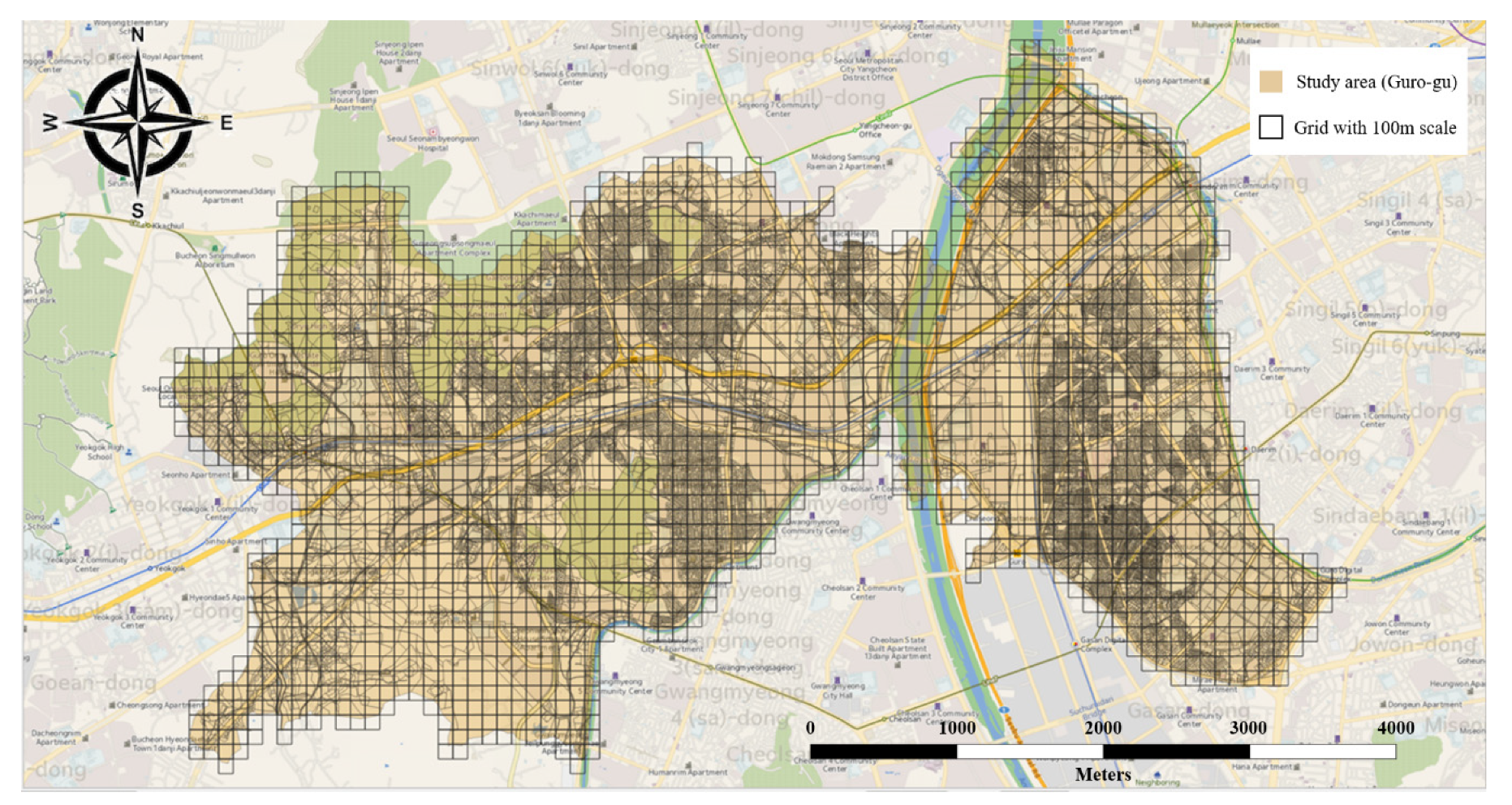
Figure 1. Study area divided by a 100 m scale grid.
Atmosphere 11 01284 g001
Figure 2. Specification of sensor-based air monitoring instrument.
Atmosphere 11 01284 g002
Figure 3. Percentage of population staying indoors by sex, age, and the time of the day in weekday. (a) Male (b) Female
Atmosphere 11 01284 g003
Figure 4. Comparison of outdoor fine particulate matter (PM2.5) concentrations modeled by a sensor-based air monitoring instrument (SAMI) and measured by an urban air monitoring station over time.
Atmosphere 11 01284 g004
Figure 5. Spatial variation of modeled outdoor PM2.5 concentration in Guro-gu.
Atmosphere 11 01284 g005
Figure 6. Correlation between outdoor PM2.5 concentrations measured by the Urban Air Monitoring Station and modeled by sensor-based air monitoring instruments in Guro-gu.
Atmosphere 11 01284 g006
Figure 7. Temporal variation of the total number of people in Guro-gu.
Atmosphere 11 01284 g007
Figure 8. Spatial variation of the total number of people in Guro-gu.
Atmosphere 11 01284 g008
Figure 9. Population exposure to PM2.5 in Guro-gu.
Atmosphere 11 01284 g009
Figure 10. Histogram of population-weighted average exposure concentrations of PM2.5.
Atmosphere 11 01284 g010
Table 1. Rate of staying indoors according to microenvironments by sex and age.
SexAgeIndoor (%)
HomeWorkplace or SchoolOther HouseRestaurant or BarOther IndoorsTransport
Male19–2499.8695.18100.0099.2587.87100
25–3499.9794.98100.0094.2483.91
35–4499.9396.66100.0096.1574.19
45–5499.9595.23100.0096.7650.60
55–6499.8292.77100.0094.9252.57
65–7499.8089.9698.7895.7152.51
<7599.4657.14100.0097.8750.86
Female19–2499.9497.45100.0097.9983.27
25–3410098.64100.0092.4632.14
35–4499.9598.02100.0098.4149.04
45–5499.9199.77100.0097.7755.70
55–6499.9595.59100.0099.6255.33
65–7499.8291.5896.8894.1270.64
<7599.76100.00100.00100.0059.60
Publisher’s Note: MDPI stays neutral with regard to jurisdictional claims in published maps and institutional affiliations.