Abstract
This study investigates the effects of atmosphere-ocean coupling for medium-range forecasts by using coupled numerical weather prediction (NWP) experiments based on the unified model (UM) on a case study of the 2016 heatwave over the Korean Peninsula. Atmospheric nudging experiments were carried out to determine the key regions which may have large impacts on the forecasts of the heat wave. The results of the nudging experiments suggest that key forcing from the Mongolia region gives the largest impact to this case by causing a transport of warm air from the northwest part of Korea. Moreover, the Pacific region shows an important role in the global circulation in nudging experiments. Results from the atmosphere-ocean coupled model show no clear benefit for the extreme heat wave temperatures in this case. In addition, more model development seems to be needed to improve the representation of sea surface temperature (SST) in some key areas. Nevertheless, it is confirmed that the atmosphere-ocean coupled simulation produces a better representation of aspects of the large-scale flow such as the blocking high over the Kamchatka Peninsula, the high pressure system in the northwest Pacific and Hadley circulation. The results presented in this study show that atmosphere-ocean coupling can be an important way to improve the deterministic model forecasts as the lead time increases beyond a few days.
1. Introduction
Extreme weather events are an area of increasing concern due to their high impacts on human society and the environment and due to the likelihood that they may change in a future climate. Therefore, forecasting extreme weather events in a timely way and with the right magnitude is clearly important for decision makers across many sectors. The Bulletin of the American Meteorological Society (BAMS) produces annual assessments of extreme weather events around the world placing them in the context of the wider climate and their impacts. The seamless prediction from weather to climate has been suggested by many as a means of reflecting the interacting processes operating continuously from weather to climate, and relevant studies of extreme weather using a wide range of prediction scales are actively performed in the international meteorological society [1,2,3]. For a long time, numerical weather prediction (NWP) systems have been based on atmosphere-only configurations with sea surface temperatures (SSTs) fixed to the initial time or varying only as initial anomalies persisted on a climatological seasonal cycle. It is known that systematic biases caused by mean state drift affect forecast performance. In order to overcome the potential limitations of atmosphere-only configured models, climate modeling has been developed by using coupled atmosphere ocean models for many years. The advantage of a unified weather and climate modeling system is that the effects of atmosphere-ocean interactions can be relatively easily evaluated in coupled models run at NWP timescales. Moreover, as supercomputer technology develops, it is possible to produce longer forecasts up to 15 days ahead for global deterministic models and provide opportunities to study the impacts of atmosphere-ocean coupling on extended medium-range forecasts.
Most operational global NWP models are atmosphere models coupled to the land surface but without the fully coupled effects of the dynamic ocean. As forecast lead times extend beyond a few days, systematic model biases begin to grow on larger spatial scales and generate difficulties in producing quantitative forecasts, generating substantial forecast errors in operational medium-range forecasts [4]. This is because these models do not reflect the interaction between atmosphere and ocean but use prescribed sea surface temperatures (SSTs). There are several studies that demonstrate the beneficial effects of coupled models for medium-range forecasts [5,6]. For instance, coupling simulations on NWP timescales have positive impacts on forecast skill for key phenomena such as Madden-Julian oscillation (MJO) [7,8,9,10,11]. In summer, the variation of SST such as cooling caused by strong wind-induced mixing influences heat flux over the ocean when tropical cyclones exist and reduces biases of track and intensity in the global coupled NWP model [12,13,14,15]. In winter, another study shows the coupled model can improve heavy snowfall simulation since SST is simulated warmer, which is more realistic. It leads to a larger supply of moisture and heat fluxes, inducing convection formation for heavy snowfall in the coastal region in the east part of Korea [16]. These studies support the consideration of atmosphere-ocean interaction in the NWP model becoming more important as the forecast time increases.
In this study we picked a heat wave case which appeared over the Korean Peninsula in August 2016 to investigate its predictability in the medium range and to explore key mechanisms in its formation and duration, including the possible effects of atmosphere-ocean coupling in the medium-range NWP forecast. The heat wave episode in August 2016 over Korea was strong and lasted for a long time (16.7 days), which broke the previous record high temperatures of 1973 [17]. According to Yeh et al. [18], the heat wave episode in August 2016 has different features compared to previous heat wave events that have typically occurred over Korea. Warm air from anomalous high pressure systems over Mongolia impacts the Korean Peninsula (Figure 1a,b), whereas adiabatic warming due to the positive geopotential height over Korea is dominant in previous heat wave events [19,20,21]. In addition, an anomalous high over the Kamchatka Peninsula induced by strong convection over the western-to-central subtropical Pacific area (Figure 1c) acts as a blocking high, which helps to maintain the heat wave for a long time.
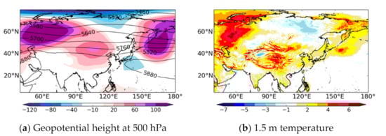
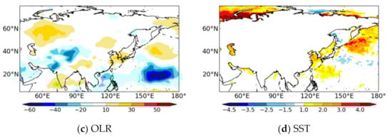
Figure 1.
(a) Anomalies of geopotential height at 500 hPa (shaded) with climatology (contour), anomalies of (b) 1.5 m temperature (K), (c) outgoing longwave radiation (OLR) (W/m2) and (d) SST (K) averaged on August 2016. Anomalies (shading) are calculated relative to the August monthly mean from 1981 to 2010. (a,b) is calculated from European Centre for Medium-Range Weather Forecasts (ECMWF) ERA-Interim atmospheric reanalysis [22] and (c) is calculated from the National Oceanic and Atmospheric Administration (NOAA) satellite-derived OLR [23]. (d) is calculated from the optimum interpolation sea surface temperature (OISST).
Since the heat wave episode in 2016 lasted for a long time, the predictability in the medium range is important. In relation to this, Ham and Na [24] investigated whether positive SST anomalies in the south sea of Korea, associated with positive geopotential height anomalies, induced warm temperature advection and less cloud amount and increased the solar radiation over Korea in the summer of 2016. In particular, they showed that this interactive response appears distinctly from a weekly timescale, reflecting that atmosphere-ocean coupling has the potential to improve medium- to extended-range forecasts.
To figure out forecast impacts on medium-range forecasts, we perform atmosphere-ocean coupled NWP simulations for our heat wave case. Before this, we investigate forecast errors of the operational global NWP model of the UK Met Office (UKMO) at that time (uncoupled to the ocean model) and explore key areas which mainly induce forecast error over the Korean Peninsula by using an atmospheric nudging technique. This technique is a useful diagnostic tool to figure out the origin of forecast error [25,26,27,28]. Then, we compare the coupled simulation results to assess whether they represent key features which the atmosphere-only simulation missed. The impact of improved model configuration using ocean coupling is thought to enhance forecast skill with potential predictability in longer timescales and also reduce model biases. Even though both are not clearly separated but mixed, this study examines both model bias and predictability responses, driven by ocean coupling.
2. Methods, Model Description and Experimental Setup
In this study, the Met Office’s unified model (MetUM) in atmosphere only and global coupled NWP models are used to investigate the effects of atmosphere-ocean coupling. We use Global Atmosphere 6.1 and Global Land 6.1 (GA6.1/GL6.1) scientific configurations [29] for the control experiment, which is consistent with the same configuration of the operational NWP system of the UKMO in 2016. For the coupled NWP model, we use the Global Climate 2.0 (GC2) [30] configuration with the nucleus for European modelling of the oceans (NEMO) dynamical ocean model [31] for the SST prediction and the Los Alamos sea ice model (CICE) [32] to predict the extent and depth of sea ice. Atmosphere/land configurations in the coupled simulation are the same as the control experiment. More details of the coupled NWP model are described in Hewitt et al. [33].
Two hindcast experiments are performed to examine the impact of atmosphere-ocean coupling. The control experiment (CTL) is the global atmosphere model, in which atmosphere and land are coupled. The coupled NWP experiment (CP) applies the effects of ocean sea ice coupling to the CTL experiment using an OASIS3 [34] coupler with the GC2 coupled science configuration. Both experiments involved multiple hindcasts, which initialized at every 00 UTC and simulated for up to 15 days for the whole of August 2016, including the heat wave target period (11–25 August). The atmosphere and land surface are initialized from operational analyses for both experiments. For the CP experiment, the ocean and sea ice fields are initialized from Met Office Ocean Forecast analysis and variables for ocean (i.e., SST, current, salinity, ice, snow etc.) to reflect the coupled NWP. The horizontal resolution of the atmosphere for both experiments is N768 (17 km in mid-latitudes). The vertical resolution of soil levels is 4 (0.1, 0.25, 0.65 and 2.0 m), and those of the atmosphere are set to 70 levels (with a top at 70 km) in both experiments. In the CP experiment, ocean levels are set to 75 levels (with a 1 m top level) and sea ice thickness categories are set to 5 (0 m, 0.6 m, 1.4 m, 2.4 m and 3.6 m). The ocean resolution of the CP experiment is 0.25° on a tri-polar grid.
To evaluate the potential remote forcing of forecast error sources over Korea from the control experiment, four nudging experiments are performed (Table 1). To evaluate forecast error source from the control experiment, four nudging experiments are performed as shown in Table 1. In the nudging code in the UM [35], the change in variable ∆X is given by
where F(X) is the rate of change in the variable due to all other factors, Xanalysisis the value of the nudged variable in the analyses, Xmodel is the value of the variable in the model and G is a relaxation parameter (6 h in this study). In this study, MetUM analysis [36] datasets are used to nudge towards the model forecast. UM analysis is datasets which are produced from the model background with a data assimilation process. Thus, it could be considered that nudged simulation is updated to a realistic field every 6 h as the forecast goes by. The dynamical prognostic variables adjusted by nudging are potential temperature (θ), zonal wind (u) and meridional wind (v). These variables are nudged on full model vertical levels at six-hourly intervals. We performed all nudging experiments at N216 (60 km in mid-latitudes) horizontal resolution to reduce computational resources since the CTL experiment reproduces a similar pattern of large-scale errors with the reduced resolution of N216 (not shown).

Table 1.
Description of nudging experiments.
In order to evaluate our experiments, we use the MetUM analysis for most of the atmospheric fields. Most results of each experiment are compared during 11–25 August 2016 when the heat wave phenomena hit the Korean Peninsula.
3. Results
This section outlines the performance of the CTL simulation in reproducing the heat wave both in terms of extreme temperatures and large-scale atmospheric circulation (Section 3.1), examines the remote forcing or forecast errors through the nudging technique (Section 3.2) and finally explores the role of atmosphere-ocean coupling in reproducing the heat wave (Section 3.3).
3.1. Diagnostic of Control Simulation
In order to investigate changes in the performance of the NWP model, spatial patterns of the variables in a 7-day forecast are examined in Figure 2, averaged over the heat wave period of 11–25 August 2016. The CTL experiment does not catch the strong high over the Kamchatka Peninsula, Western Eurasia, East China and Mongolia (Figure 2a), and consequently overestimates horizontal winds at 200 hPa due to the failure to capture blocking over the Kamchatka Peninsula (Figure 2c). In addition, the CTL simulation underestimates the 500 hPa geopotential height in the northwestern Pacific area, south of Japan at 25° N. During the simulation period, six typhoons occurred in this northwestern Pacific region and the CTL experiment simulates typhoons stronger than the analysis, which is consistent with the negative bias in the time-mean at 500 hPa geopotential height [6,12]. For outgoing longwave radiation (OLR), the CTL experiment produces stronger convection (negative error in OLR) over the western-central Pacific region and east of the Philippines (Figure 2d), which is also pointed out by Yeh et al. [18] as a remote trigger region for blocking over the Kamchatka Peninsula. It is also shown that the CTL simulation produces a stronger Hadley circulation compared to the analysis (Figure 3). This is related to the excessive convection and diabatic heating over some of the oceanic areas shown in Figure 2d.
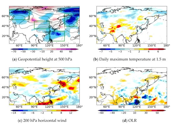
Figure 2.
Biases for the 7-day forecast averaged during heat wave period (11–25 August 2016) for (a) 500 hPa geopotential height (m), (b) daily maximum temperature at 1.5 m (K), (c) 200 hPa horizontal wind (m/s) and (d) OLR (Wm−2). Biases are against Met Office’s unified model (MetUM) analysis and boxed areas in (a) represent areas for nudged experiments described in Section 2.
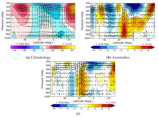
Figure 3.
Zonal U wind (contour and shading) and meridional-omega wind vector for (a) climatology (August monthly mean from 1981 to 2010), (b) anomalies for August 2016 and (c) biases for the 7-day forecast in the control experiment (CTL) experiment averaged during August 2016. All values are averaged 120° E–140° E.
From the features 500 hPa geopotential height, 200 hPa horizontal wind and OLR, we can guess that the CTL experiment does not simulate the Korean heat wave well because it does not forecast features of important areas that Yeh et al. [18] pointed out—the Kamchatka peninsula, Mongolia and the west subtropical Pacific. As seen in Figure 2b, the CTL simulation produces cold biases of up to −3 K to −5 K over the whole area of South Korea. Therefore, we choose four areas in Table 1, marked in Figure 2a, for forecast error sources and a nudging experiment is performed.
We compared the forecasting skill between the different lead time simulations in key areas of Table 1. For the target period, the daily maximum temperatures for short-range forecasts (up to 4 days) are very close to the analysis in daily tendencies although cold biases appear over Korea (Figure 4a). However, the agreement in daily tendency reduces as the forecast lead time becomes longer. The forecast for the high pressure shows good skill in the timescale shorter than 4 days. As the forecast lead time increases to 7 days, high pressures over the Kamchatka Peninsula, Mongolia and the west subtropical Pacific are underestimated (Figure 4b–d). In addition, there is a big temperature drop on 20th August in the CTL experiment at the 7-day forecast. It is remarkable that a big drop of geopotential height over the Kamchatka Peninsula appears 2 days before the cold bias occurs (Figure 4b). A similar pattern is shown over the west subtropical Pacific as well, although the magnitude of the change is small compared to the Kamchatka Peninsula (Figure 4d). While the cold bias grows over South Korea at the 7-day forecast, high pressure of 500 hPa geopotential height over Mongolia is also largely underestimated in the CTL simulation (Figure 4c). From this, we can infer that biases from these areas may contribute to the failure to forecast the heat wave over South Korea.
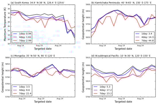
Figure 4.
(a) Time series of daily maximum temperature (°C) averaged over South Korea in the CTL experiment at each forecast day (day 1, day 4 and day 7) with the MetUM analysis (black). (b–d) are time series of 500 gph height averaged over (b) the Kamchatka Peninsula (40° N–65° N, 150° E–175° E) (c) Mongolia (35° N–50° N, 90° E–125° E) and (d) the northwest Pacific (10° N–30° N, 120° E–150° E) in the CTL experiment at each forecast day (day 1, day 4 and day 7) with the MetUM analysis (black). Numbers in the box are the root mean square error (RMSE) at each forecast lead time.
3.2. Nudged Simulation
In order to investigate the potential effect of each area on remotely forcing the cold biases over South Korea, the results of nudged experiments are shown in Figure 5 and Figure 6 and Table 2. During the heat wave event period, there is high pressure over East China and warm advection-related flows toward Korea (Figure 5a). The CTL experiment (at N216 resolution) reproduces the cold biases over the Korean Peninsula and weak high pressure biases in south of Korea (Figure 5b). In the fully global nudged experiment, cold biases are largely reduced. This is because transport of warm air from the northwest of Korea is increased due to anti-cyclonic circulation induced by stronger high pressures in East China (Figure 5c). In addition to the global nudged experiment, Mongolia nudged (MO) and Pacific nudged (PA) experiments also reproduce the observed high pressure over East China and reduced temperature bias (Figure 5d,e or Figure 6a). In particular, the MO experiment gives the largest impacts over the Korean Peninsula by reducing temperature biases. This is because temperature biases are reduced in Mongolia by the nudging effect, and the strength of the high pressure in Southeast China is also well represented (Figure 5d or Figure 6b). It is shown that the nudged experiment of the northwest Pacific region also reduces temperature biases over the Korean Peninsula (Figure 5e or Figure 6a). The reason that the PA experiment reduces cold biases over Korea is due to a stronger high pressure in East China induced by accurate reproducing of the low pressure in the south of Japan (Figure 5e or Figure 6b). The reduction of cold biases, however, is not large compared to the MO experiment because cold biases still exist north of Korea, hence transport of warm air does not occur in the PA experiment. In summary, to reduce the cold bias over Korea, an accurate forecast of the circulation northwest of Korea (i.e., Mongolia) is more important than the northwestern Pacific high in this case. All nudged experiments reduce biases for other variables around Korea (Table 2), however, nudged experiments for Western Eurasia and the Kamchatka Peninsula do not produce large impacts on heat wave phenomena (Figure 5f,g).
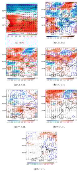
Figure 5.
(a) 500 hpa geopotential height (contour), 1000 hPa temperature (°C, shaded) and 850 hPa wind (vector) of ERA Interim reanalysis (ERAI), (b) 7-day forecasted 500 hPa geopotential height (contour, blue and red line represent positive and negative bias, respectively), biases for the 7-day forecasted 850 hPa wind (vector) and 1000 hPa temperature (shaded) in the CTL experiment. (c–g) Differences of 7-day forecasted 500 hPa geopotential height (contour), 850 hPa wind (vector) and 1000 hPa temperature (shaded) between each experiment and the CTL experiment. Biases are calculated with the MetUM analysis. All values are averaged during the heat wave period (11–25 August 2016).
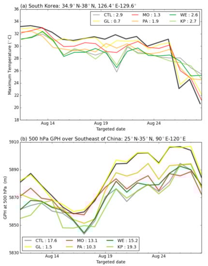
Figure 6.
Time series of the 7-day forecast maximum temperature (°C) in each nudged experiment averaged over (a) South Korea (34.9° N–38° N, 126.4° E–129.6° E) with the MetUM analysis (black line) and (b) 500 hPa geopotential height over Southwest China (25° N–35° N, 90° E–120° E) with the MetUM analysis (black line). Numbers in box mean averaged RMSE of each experiment.
Table 2.
RMSE of 7-day forecasts of each nudged experiment for three variables. Values are averaged around Korea (25° N–50° N, 115° E–140° E).
Although the PA experiment gives smaller impacts for the heat wave compared to the MO experiment, it is remarkable that the PA experiment represents Hadley circulation fairly well by producing opposite signals compared to the CTL experiment (Figure 3c or Figure 7f). When compared with the MO experiment, the PA experiment gives a large impact outside the nudged region (Figure 7e) as well as in the nudged area (Figure 7f), whereas the MO experiment gives smaller impacts outside the nudged area (Figure 7d). It implies that the Pacific region has an important role in global circulation.
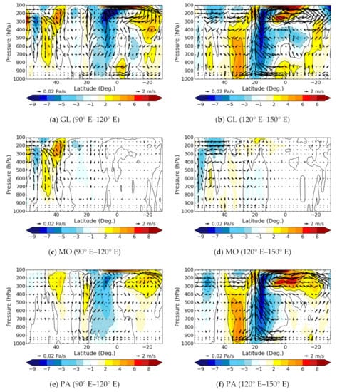
Figure 7.
Differences in 7-day forecasted fields of zonal U wind (contour and shading) and meridional-omega wind vector between each experiment ((a,b) for GL, (c,d) for MO and (e,f) for PA) and the CTL experiment averaged during the heat wave period (11–25 August 2016). (a,c,e) are averaged between 90° E–120° E (same longitude with MO experiment) and (b,d,f) are averaged 120° E–150° E (same longitude with PA experiment).
The key areas for the Korean heat wave identified in Yeh et al. [18] are well matched with the results of the nudged experiments and the identified forecast remote error sources. As a next step, we hypothesize that the coupled NWP simulation could potentially reduce biases of the CTL experiment if it captures the atmospheric patterns over the northwestern Pacific and Mongolia. In addition, the SST could also have a local effect on the heat wave. Since the CTL experiment does not simulate the SST during the forecast lead time when the SST anomaly is high around the Korean peninsula (Figure 1d), it could be another factor in the failure of predictions to fully capture the heat wave phenomena.
3.3. Impact of Atmosphere-Ocean Coupling
Coupled NWP simulations are carried out in an attempt to improve forecast skill for the above-mentioned key areas of the Korea heat wave forecast. Impacts of coupled NWP are compared with the CTL experiment, as shown in Figure 8 and Figure 9. Figure 8 depicts the differences in each variable between the CP experiment and the CTL experiment averaged during the targeted heat wave period at 7-day forecast lead times onwards. Figure 9 shows comparisons between the CTL experiment and CP experiment at each forecast date, as in Figure 4. Except for some land areas in Figure 8a, differences between the CTL and the CP experiments are not large over land. The CP experiment does not show better performance for daily maximum temperature although it reduces the cold peak errors in the middle of the heat wave (20th or 21st August) compared to the CTL run (Figure 8a), whereas it reduces temperature biases from the CTL experiment in the oceanic area (Figure 8b vs. Figure 2b). These results are consistent with earlier results in that the CP simulation does not give significant improvement over the key region of Mongolia (Figure 8a or Figure 9c). Although reductions of errors in Mongolia are not visible in the 7-day forecast, the CP experiment gives better scores in Mongolia during the early-mid stage of the heat wave and cold biases are decreased during this period in the 10-day forecast (Figure 9a,c). On the other hand, differences between the CTL and the CP experiment are small when the earlier forecast lead time is before day 1 (not shown). This suggests that the influence of the ocean coupling takes time to impact on the circulation over land and is felt at later forecast ranges beyond week 1.
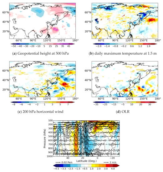
Figure 8.
Differences between averaged 7-day forecast CP and CTL experiments (CP-CTL) for (a) 500 hPa geopotential height (m), (b) daily maximum temperature at 1.5 m (K), (c) 200 hPa horizontal wind (m/s), (d) OLR (W/m2) and (e) zonal winds as in Figure 7. Averaging period is 11–25 August 2016.
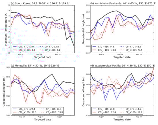
Figure 9.
(a) Time series of daily maximum temperature (°C) averaged over South Korea in the CTL (solid line) and the CP (dashed line) experiments at each forecast day (blue for day 7, red for day 10) with the MetUM analysis (black). (b–d) are time series of 500 gph height averaged over (b) the Kamchatka Peninsula (40° N–65° N, 150° E–175° E) (c) Mongolia (35° N–50° N, 90° E–125° E) and (d) the northwest Pacific (10° N–30° N, 120° E–150° E) in the CTL experiment (solid line) and the CP (dashed line) experiments at each forecast day (blue for day 7, red for day 10) with the MetUM analysis (black). Numbers in the box are the root mean square error (RMSE) at each forecast lead time.
Despite the neutral impacts for land areas at day 7, the CP experiment generally tends to produce a better forecast tendency than the CTL experiment in oceanic areas. Near the Kamchatka Peninsula, biases in the 7-day forecasts are reduced in the coupled simulation (Figure 8a) and improvement occurs especially during the early stage of the heat wave (11–13 August in Figure 9b). At the 7-day forecast range, more improvements occur in the CP experiment although there is a negative peak on the 17th of August. This means that the significance of air-sea coupling becomes important as the forecast lead time becomes longer [6,9,11,13,37].
In the subtropical west Pacific, a remarkable enhancement appears in the coupled simulation and impacts are larger as the forecast time increases (Figure 9d). Large reductions of errors in air-sea coupling simulation are mainly shown over oceanic areas in 200 hPa horizontal wind and OLR (Figure 8c,d and contrast with error structures in Figure 2c,d). For these variables, biases for 7-day forecasts of the coupled simulation are decreased, especially in the oceanic area, as shown by the opposite sign compared to those of the CTL experiment. In addition, strong Hadley circulation bias simulated in the CTL is reduced (Figure 8e compared to Figure 3c). This is similar to features in the PA nudged experiment. This means that impacts of atmosphere-ocean coupling give positive impacts to the global circulation field again via changes in convection and diabatic heating over tropical oceanic regions.
The positive impacts of coupling are confirmed in the RMSE changes of 500 hPa geopotential height, 200 hPa horizontal wind and OLR in the CP experiment of Figure 10. RMSE is reduced in the extended range forecast in the global scale and locally over East Asia as well. Reductions of RMSEs are generally larger over the ocean than land areas. According to Figure 10, the positive effects of the coupled NWP run are larger in atmospheric circulation than temperature. These results are consistent with Lea et al. [38], who described that improvement of large-scale dynamic fields (winds and pressure) appeared whereas temperature fields were degraded using the Hadley Centre Global Environment Model version 3 (HadGEM3) coupled forecast model.
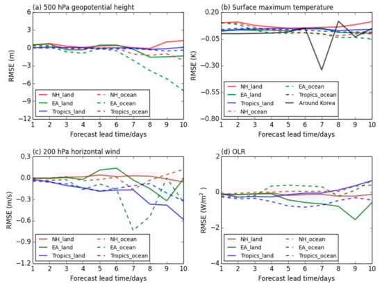
Figure 10.
Differences of RMSE between the CP and the CTL experiments (CP-CTL) in (a) 500 hPa geopotential height (m), (b) daily maximum temperature at 1.5 m (K), (c) 200 hPa horizontal wind (m/s) and (d) OLR (W/m2) at each forecast lead time averaged over each area (northern hemisphere: 20° N–90° N, tropic: 20° S–20° N and East Asia: 25° N–70° N, 90° E–180° E, around Korea: 25° N–50° N, 115° E–140° E) during the targeted case period (11–25 August 2016). Contour (dashed) line means averaged value over ocean (land) area of each region. Negative values mean that the CP experiment reduces RMSE compared to the CTL experiment.
A big difference between atmosphere-ocean coupling and uncoupled simulation is that SST is forecasted from the model rather than being fixed at values from the initialization time. SST is a typical variable which impacts directly from ocean to atmosphere. In the CTL experiment, there are cold biases in the south of the Bering Sea and warm biases in the Okhotsk Sea and northwest part of the Pacific for the 7-day forecast (Figure 11a). There are also significant biases along the Asian-Arctic coastline. SSTs reproduced by the CP experiment alleviate biases over the tropical Pacific region and higher latitude (including Bering Sea and Okhotsk Sea) (Figure 11b,c or Figure 12a). It shows the advantage of air-sea coupling processes in the NWP forecasts mentioned in previous studies. The evolution of SSTs in coupled and uncoupled forecasts (Figure 12a) clearly confirm that the CP experiment simulates a more realistic SST distribution in the Bering Sea region. In addition, a strong SST signal is associated with a stronger high pressure system over the Kamchatka peninsula in the CP experiment (Figure 8a or Figure 11a). These results reflect that a better SST condition in the CP simulation modulates meridional circulation and potentially reduces model drifts.
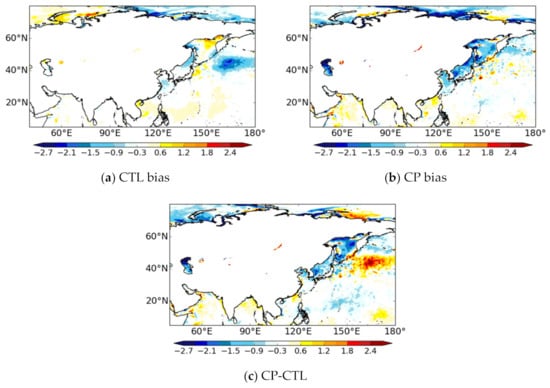
Figure 11.
Bias of SST (K) in the (a) CTL experiment and (b) CP experiment. (c) Differences of SST between the CP and the CTL experiment (CP minus CTL). Biases are calculated from the operational sea surface temperature and sea ice analysis (OSTIA) data [40]. Both experiments are 7-day forecasts and averaged during 11–25 August 2016.
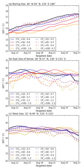
Figure 12.
Same as Figure 6, but for daily SST (°C) averaged over (a) Bering Sea (40° N–50° N, 155° E–180° E) (b) East Sea (32° N–40° N, 120° E–135° E) and (c) West Sea of Korea (32° N–40° N, 120° E–125° E). The black line represents OSTIA analysis and RMSEs are calculated using OSTIA. The reason of the shift at the 1-day forecast in the CTL experiment is that the CTL experiment uses the previous day’s SST value.
However, the CP experiment shows limited forecast performance in more local coastal regions. Excessive cold biases of SST appear around Korea as the forecast lead time increases (Figure 12b,c). Cooler SST in the CP experiment induces a decrease in surface heat fluxes (Figure 13e) and the PBL depth (not shown) over areas where cold biases appear (e.g., Figure 10 of Yamamoto and Hirose [39]). These local cold SST biases could impact the temperature of the Korean Peninsula.
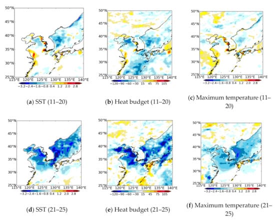
Figure 13.
Differences between the CP and CTL experiment (CP minus CTL) for (a,d) SST (K), (b,e) heat budget (Wm-2) and (c,f) daily maximum temperature (K). (a–c) are averaged during 11–20 and (d–f) are averaged during 21–25 August 2016. All experiments are forecasted at 7 days before the targeted time. The heat budget is calculated by the sum of net downward longwave radiation flux, net downward shortwave radiation flux and latent and sensible heat fluxes.
In relation to this, Figure 9a shows that the 7-day forecasts of the CP experiment reproduce similar or better representation for maximum temperature over Korea until the 21th of August, whereas it produces cooler values after that. This can be related to extremely cold SSTs around Korea being produced in the CP experiment several days before the 21th of August (Figure 12b,c or Figure 13d). We compared mean fields of each experiment between 11–20 and 21–25 August, as shown in Figure 13. The colder local SST during 21–25 in the CP experiment (Figure 13a,d) reduces more heat fluxes to the atmosphere (Figure 13b,e). It enables increased cloud amount (not shown) and leads to increased cold biases in the daily maximum temperature (Figure 13c,f).
In summary, another factor which causes a failure of the heat wave predictions over the Korean Peninsula in the coupled simulations might be the cooler SSTs in the local coastal region surrounding Korea. Generally, coupled models have benefits by reproducing more realistic SSTs than uncoupled models [14,41,42,43]. In addition, the coupled NWP model represents better SSTs around Korea in other cases [43,44]. However, there is also a possibility that small fluctuation grows rapidly. Lea et al. [38] suggests future areas for improvement being the diurnal cycle of SST and river runoff. Regarding coastal regional performance such as around the Korean Peninsula, diurnal variations of temperature need to be investigated to figure out the effects of atmosphere-ocean coupling.
From these results, it can be inferred that more investigation and study about SST near the Korean Peninsula are needed to figure out the reasons for the overcooling in the coupled NWP model. Results of additional simulations not included in this paper show that if SSTs are represented correctly as observed, then daily maximum temperature biases over Korea could be further reduced.
Although the CP experiment does not fully capture the heat wave phenomena over the Korean Peninsula and overcooled SSTs appear near the Korean peninsula for this case, it does generally improve the overall forecast results in the East Asian and West Pacific regions by better capturing the synoptic scale features and the global-scale circulation. These results can support the necessity of reflecting the atmosphere-ocean coupling in medium-range forecasts.
4. Concluding Remarks
As the number of severe weather events which are difficult to predict are increasing, the accuracy of numerical forecast models which cover various timescales becomes more important. A NWP model based on atmosphere-only configurations has limitations in simulating interactive atmosphere-ocean processes potentially important at extended forecast ranges. Currently, including a coupled ocean into weather forecast models for NWP timescales can be difficult due to limited computing resources. However, coupling with the ocean and sea ice model, used for seasonal and longer time scales, is known to give benefits in medium range forecasts in NWP timescales [6,9,23,37,38]. Motivated by these previous studies, the effects of atmosphere-ocean coupling for an extreme heat wave over Korea during August 2016 are investigated using the MetUM coupled with the NWP model. The heat wave of 2016 lasted for about 16 days. A cold bias growing in operational medium-range forecasts made during the heat wave was an important issue in delivering advice on the heat wave duration and intensity.
Major regions affecting forecast skill during the heat wave episode were investigated using atmospheric nudging experiments. Results of the nudging simulations show that Mongolia and the northwestern Pacific area give large impacts on forecasts. These two experiments enhance high pressure systems over Southeast China and the Bering Sea (not shown). Having identified these key regions, the question was posed whether a coupled NWP simulation could improve these areas, in which case we might expect an improved heat wave forecast over the Korean Peninsula compared to the non-coupled model.
Results of coupled NWP runs do alleviate synoptic errors especially over the oceanic areas. Reduced systematic biases result in improving performance on longer timescales, as coupling effects are visible from day 7 onward. Coupling effects are also significant in high latitudes as well as the tropics. Systematic biases over the Kamchatka Peninsula are reduced. This is because atmosphere-ocean interaction improves the representation of the global circulation. The positive effect of the coupled run is larger in atmospheric circulation than daily maximum temperature. The coupled simulation gives little benefits for extreme heat wave temperatures over the Korean Peninsula. Reducing model error over Mongolia in nudged runs gives the largest impact on the Korean heat wave. The Mongolian errors in the control run are not impacted in the coupled NWP model, whereas biases over the northwestern Pacific area are visibly reduced. Another factor in the coupled simulation that does not improve the Korean heat wave seems to be excessive cooling of the SST around the Korean Peninsula. This is an area requiring further investigation.
The impact of air-sea coupling on weather forecasting systems has shown positive benefits in other extreme weather cases (i.e., typhoon, MJO) using similar frameworks to this study [8,12,37,43]. Therefore, our results have confirmed skillful representation for the medium-range from coupling over the oceanic regions and for the large-scale atmospheric circulation (e.g., blocking high over the Kamchatka Peninsula, high pressure system in northwest Pacific and Hadley circulation). Meanwhile, some degradation in SST bias is found in the coastal region surrounding Korea from coupling the atmosphere to a dynamic ocean model. Including these issues, there are also still many topics to improve the skill of the coupled NWP model, i.e., developing data assimilation for coupled NWP to alleviate initialization shock [38,45] and using higher resolution models in both atmosphere and ocean to improve representation of extreme and hazardous weather [46].
This study supports the use of coupled NWP in medium-range forecasts by showing decreased systematic errors and skillful results due to reduced mean state drift. However, many more detailed and process-based case studies are needed to fully investigate the effects of coupled models at NWP timescales and promote further coupled model developments to enhance the forecast skill in the medium range.
Author Contributions
E.-J.K. and C.M. conceived and designed the experiments; E.-J.K. performed the experiments and E.-J.K., C.M. and S.F.M. contributed to analyzed the data; E.-J.K. wrote the initial manuscript; K.-O.B. modified the manuscript; Y.K., J.O. and H.-S.K. contributed to manuscript improvement and revisions. All authors have read and agreed to the published version of the manuscript.
Funding
This research was supported by the Numerical Modeling Center of the Korea Meteorological Administration under grant number KMA2018-00721, “Development of Numerical Weather Prediction and Data Application Techniques”.
Acknowledgments
The authors would like to thank the anonymous reviewers for insightful comments that have made this a better paper.
Conflicts of Interest
The authors declare no conflict of interest.
References
- Cassou, C.; Terray, L.; Phillips, A.S. Tropical Atlantic influence on European Heat Waves. J. Clim. 2005, 18, 2805–2811. [Google Scholar] [CrossRef]
- Brunet, G.; Hoskins, M.; Moncrieff, M.; Dole, R.; Kiladis, G.N.; Kirtman, B.; Lorenc, A.; Mills, B.; Morss, R.; Polavarapu, S.; et al. Collaboration of the weather and climate communities to advance subseasonal-to-seasonal prediction. Bull. Amer. Meteor. Soc. 2010, 91, 1397–1406. [Google Scholar] [CrossRef]
- Bretherton, C.; Balaji, V.; Delworth, T.; Dickinson, R.E.; Edmonds, J.A.; Famiglietti, J.S.; Smarr, L.L. A National Strategy for Advancing Climate Modeling; The National Academies Press: Washington, DC, USA, 2012; pp. 197–208. [Google Scholar]
- Jung, T.; Tompkins, A.M.; Rodwell, M.J. Some aspects of systematic error in the ECMWF model. Atmos. Sci. Lett. 2005, 6, 133–139. [Google Scholar] [CrossRef]
- Buizza, R.; Balsamo, G.; Haiden, T. IFS upgrade brings more seamless coupled forecasts. ECMWF Newsl. 2018, 156, 18–22. [Google Scholar]
- Smith, G.C.; Bélanger, J.M.; Roy, F.; Pellerin, P.; Ritchie, H.; Onu, K.; Roch, M.; Zadra, A.; Colan, D.S.; Winter, B.; et al. Impact of coupling with an ice−ocean model on global medium-range NWP forecast skill. Mon. Weather Rev. 2018, 46, 1157–1180. [Google Scholar] [CrossRef]
- DeMott, C.A.; Klingaman, N.P.; Woolnough, S.J. Atmosphere-ocean coupled processes in the Madden-Julian oscillation. Rev. Geophys. 2015, 53, 1099–1154. [Google Scholar] [CrossRef]
- Shelly, A.; Xavier, P.; Copsey, D.; Johns, T.; Rodriguez, J.M.; Milton, S.; Klingaman, N. Coupled versus uncoupled hindcast simulations of the Madden–Julian Oscillation in the Year of Tropical Convection. Geophys. Res. Lett. 2014, 41, 5670–5677. [Google Scholar] [CrossRef]
- Fu, X.; Wang, B. Differences of Boreal Summer Intraseasonal Oscillations Simulated in an Atmosphere–Ocean Coupled Model and an Atmosphere-Only Model. J. Clim. 2004, 17, 1263–1271. [Google Scholar] [CrossRef]
- Feng, X.; Haines, K.; Liu, C.; de Boisséson, E.; Polo, I. Improved SST–precipitation intraseasonal relationships in the ECMWF coupled climate reanalysis. Geophys. Res. Lett. 2018, 45, 3664–3672. [Google Scholar] [CrossRef]
- Park, S.; Kim, D.J.; Lee, S.W.; Lee, K.W.; Kim, J.; Song, E.J.; Seo, K.H. Comparison of extended medium-range forecast skill between KMA ensemble, ocean coupled ensemble, and GloSea5. Asia-Pac. J. Atmos. Sci. [CrossRef]
- Feng, X.; Klingaman, N.P.; Hodges, K.I. The effect of atmosphere–ocean coupling on the prediction of 2016 western North Pacific tropical cyclones. Q. J. R. Meteorol. Soc. 2019, 145, 2425–2444. [Google Scholar] [CrossRef]
- Ito, K.; Kuroda, T.; Saito, K.; Wada, A. Forecasting a Large Number of Tropical Cyclone Intensities around Japan Using a High-Resolution Atmosphere–Ocean Coupled Model. Weather Forecast. 2015, 30, 793–808. [Google Scholar] [CrossRef]
- Ren, X.; Perrie, W.; Long, Z.; Gyakum, J. Atmosphere–Ocean Coupled Dynamics of Cyclones in the Midlatitudes. Mon. Weather Rev. 2004, 132, 2432–2451. [Google Scholar] [CrossRef]
- Mogensen, K.S.; Magnusson, L.; Bidlot, J.R. Tropical cyclone sensitivity to ocean coupling in the ECMWF coupled model. J. Geophys. Res. Ocean. 2017, 122, 4392–4412. [Google Scholar] [CrossRef]
- Kim, T.; Jin, E.K. Impact of an interactive ocean on numerical weather prediction: A case of a local heavy snowfall event in eastern Korea. J. Geophys. Res. Atmos. 2016, 121, 8243–8253. [Google Scholar] [CrossRef]
- KMA. Weather Characteristic in August 2016. Korea Meteorol. Adm. Rep.. 2016. Available online: http://web.kma.go.kr/notify/press/kma_list.jsp?bid=press&mode=view&num=1193250&page=11&field=&text= (accessed on 22 March 2020).
- Yeh, S.Y.; Won, Y.J.; Hong, J.S.; Lee, K.J.; Kwon, M.; Seo, K.H.; Ham, Y.G. The Record-Breaking Heat Wave in 2016 over South Korea and Its Physical Mechanism. Mon. Weather Rev. 2018, 146, 1463–1474. [Google Scholar] [CrossRef]
- Lee, W.S.; Lee, M.I. Interannual variability of heat waves in South Korea and their connection with large-scale atmospheric circulation patterns. Int. J. Climatol. 2016, 36, 4815–4830. [Google Scholar] [CrossRef]
- Yeo, S.R.; Yeh, S.W.; Lee, W.S. Two types of heat wave in Korea associated with atmospheric circulation pattern. J. Geophys. Res. Atmos. 2019, 124, 7498–7511. [Google Scholar] [CrossRef]
- Kim, H.K.; Moon, B.K.; Kim, M.K.; Kwon, M. Dynamic mechanisms of summer Korean heat waves simulated in a long-term unforced Community Climate System Model version 3. Atmos. Sci. Lett. 2020, 21, e973. [Google Scholar] [CrossRef]
- Dee, D.P.; Uppala, S.M.; Simmons, A.J.; Berrisford, P.; Poli, P.; Kobayashi, S.; Andrae, U.; Balmaseda, M.A.; Balsamo, G.; Bauer, P.; et al. The ERA-Interim reanalysis: Configuration and performance of the data assimilation system. Q. J. R. Meteorol. Soc. 2011, 137, 553–597. [Google Scholar] [CrossRef]
- Liebmann, B.; Smith, C.A. Description of a complete (interpolated) outgoing long wave radiation dataset. Bull. Am. Meteor. Soc. 1996, 77, 1275–1277. [Google Scholar]
- Ham, Y.G.; Na, H.Y. Marginal sea surface temperature variation as a pre-cursor of heat waves over the Korean Peninsula. Asia-Pac. J. Atmos. Sci. 2017, 53, 445–455. [Google Scholar] [CrossRef]
- Klinker, E. Investigation of systematic errors by relaxation experiments. Q. J. R. Meteorol. Soc. 1990, 116, 573–594. [Google Scholar] [CrossRef]
- Jung, T.; Miller, M.J.; Palmer, T.N. Diagnosing the origin of extended-range forecast errors. Mon. Weather Rev. 2010, 138, 2434–2446. [Google Scholar] [CrossRef]
- Jung, T.; Palmer, T.N.; Rodwell, M.J.; Serrar, S. Understanding the anomalously cold European winter of 2005/06 using relaxation experiments. Mon. Weather Rev. 2010, 138, 3157–3174. [Google Scholar] [CrossRef]
- Rodríguez, J.M.; Milton, S.F. East Asian Summer Atmospheric Moisture Transport and Its Response to Interannual Variability of the West Pacific Subtropical High: An Evaluation of the Met Office Unified Model. Atmosphere 2019, 10, 457. [Google Scholar] [CrossRef]
- Walters, D.; Brooks, M.; Boutle, I.; Melvin, T.; Stratton, R.; Vosper, S.; Wells, H.; Williams, K.; Wood, N.; Allen, T.; et al. The Met Office Unified Model Global Atmosphere 6.0/6.1 and JULES Global Land 6.0/6.1 configurations. Geosci. Model. Dev. 2017, 10, 1487–1520. [Google Scholar] [CrossRef]
- Williams, K.D.; Harris, C.M.; Bodas-Salcedo, A.; Camp, J.; Comer, R.E.; Copsey, D.; Fereday, D.; Graham, T.; Hill, R.; Hinton, T.; et al. The Met Office Global Coupled model 2.0 (GC2) configuration. Geosci. Model Dev. 2015, 8, 1509–1524. [Google Scholar] [CrossRef]
- Megann, A.; Storkey, D.; Aksenov, Y.; Alderson, S.; Calvert, D.; Graham, T.; Hyder, P.; Siddorn, J.; Sinha, B. GO5.0: The joint NERC–Met Office NEMO global ocean model for use in coupled and forced applications. Geosci. Model Dev. 2014, 7, 1069–1092. [Google Scholar] [CrossRef]
- Rae, J.G.L.; Hewitt, H.T.; Keen, A.B.; Ridley, J.K.; West, A.E.; Harris, C.M.; Walters, D.N. Development of the Global Sea Ice 6.0 CICE configuration for the Met Office Global Coupled model. Geosci. Model Dev. 2015, 8, 2221–2230. [Google Scholar] [CrossRef]
- Hewitt, H.T.; Copsey, D.; Culverwell, I.D.; Harris, C.M.; Hill, R.S.R.; Keen, A.B.; McLaren, A.J.; Hunke, E.C. Design and implementation of the infrastructure of HadGEM3: The next generation Met Office climate modelling system. Geosci. Model Dev. 2011, 4, 223–253. [Google Scholar] [CrossRef]
- Valcke, S. The OASIS3 coupler: A European climate modelling community software. Geosci. Model Dev. 2013, 6, 373–388. [Google Scholar] [CrossRef]
- Telford, P.J.; Braesicke, P.; Morgenstern, O.; Pyle, J.A. Technical Note: Description and assessment of a nudged version of the new dynamics Unified Model. Atmos. Chem. Phys. 2008, 8, 1701–1712. [Google Scholar] [CrossRef]
- Clayton, A.M.; Lorenc, A.C.; Barker, D.M. Operational implementation of a hybrid ensemble/4D-Var global data assimilation system at the Met Office. Q. J. R. Meteorol. Soc. 2013, 139, 1445–1461. [Google Scholar] [CrossRef]
- Johns, T.; Shelly, A.; Rodriguez, J.; Copsey, D.; Guiavarc’h, C.; Waters, J.; Sykes, P. Report on extensive coupled ocean-atmosphere trials on NWP (1–15 day) timescales. PWS Key Deliv. Rep. 2012, 29, 56. [Google Scholar]
- Lea, D.; Mirouze, I.; Martin, M.; King, R.; Hines, A.; Walters, D.; Thurlow, M. Assessing a new coupled data assimilation system based on the Met Office coupled atmosphere–land–ocean–sea ice model. Mon. Weather Rev. 2015, 143, 4678–4694. [Google Scholar] [CrossRef]
- Yanamoto, M.; Hirose., N. Regional atmospheric simulation of monthly precipitation using high-resolution SST obtained from an ocean assimilation model: Application to the wintertime Japan Sea. Mon. Weather Rev. 2009, 137, 2164–2174. [Google Scholar] [CrossRef]
- Craig, J.D.; Matthew, M.; John, S.; Jonah, R.-J.; Emma, F.; Werenfrid, W. The Operational Sea Surface Temperature and Sea Ice Analysis (OSTIA) system. Remote Sens. Environ. 2012, 116, 140–158. [Google Scholar]
- Yang, B.; Zhang, Y.; Qian, Y.; et al. Better monsoon precipitation in coupled climate models due to bias compensation. NPJ Clim. Atmos. Sci. 2019, 2, 43. [Google Scholar] [CrossRef]
- Thompson, B.; Sanchez, C.; Sun, X.; Song, G.; Liu, J.; Huang, X.-Y.; Tkalich, P. A high-resolution atmosphere–ocean coupled model for the western Maritime Continent: Development and preliminary assessment. Clim. Dyn. 2019, 52, 3951–3981. [Google Scholar] [CrossRef]
- Shelly, A.; Johns, T.; Rodríguez, J.; Thorpe, L.; Copsey, D. Assessing the Physical Mechanisms for Improved Skill of Coupled NWP Forecasts on 1–15 Day Lead Times for Both Tropical and Extra-Tropical Air-Sea Interactions; PWS Key Deliverable Report; Met Office: Exeter, UK, 2015; Volume 32. [Google Scholar]
- Iwasaki, S.; Isobe, A.; Kako, S. Atmosphere–Ocean Coupled Process along Coastal Areas of the Yellow and East China Seas in Winter. J. Clim. 2014, 27, 155–167. [Google Scholar] [CrossRef]
- Mulholland, D.P.; Laloyaux, P.; Haines, K.; Balmaseda, M.A. Origin and impact of initialization shocks in coupled atmosphere–ocean forecasts. Mon. Weather Rev. 2015, 143, 4631–4644. [Google Scholar] [CrossRef]
- Bryan, F.O.; Tomas, R.; Dennis, J.M.; Chelton, D.B.; Loeb, N.G.; McClean, J.L. Frontal scale air–sea interaction in high-resolution coupled climate models. J. Clim. 2010, 23, 6277–6291. [Google Scholar] [CrossRef]


Publisher’s Note: MDPI stays neutral with regard to jurisdictional claims in published maps and institutional affiliations. |
© 2020 by the authors. Licensee MDPI, Basel, Switzerland. This article is an open access article distributed under the terms and conditions of the Creative Commons Attribution (CC BY) license (http://creativecommons.org/licenses/by/4.0/).