Abstract
Extreme precipitation is no longer stationary under a changing climate due to the increase in greenhouse gas emissions. Nonstationarity must be considered when realistically estimating the amount of extreme precipitation for future prevention and mitigation. Extreme precipitation with a certain return level is usually estimated using extreme value analysis under a stationary climate assumption without evidence. In this study, the characteristics of extreme value statistics of annual maximum monthly precipitation in East Asia were evaluated using a nonstationary historical climate simulation with an Earth system model of intermediate complexity, capable of long-term integration over 12,000 years (i.e., the Holocene). The climatological means of the annual maximum monthly precipitation for each 100-year interval had nonstationary time series, and the ratios of the largest annual maximum monthly precipitation to the climatological mean had nonstationary time series with large spike variations. The extreme value analysis revealed that the annual maximum monthly precipitation with a return level of 100 years estimated for each 100-year interval also presented a nonstationary time series which was normally distributed and not autocorrelated, even with the preceding and following 100-year interval (lag 1). Wavelet analysis of this time series showed that significant periodicity was only detected in confined areas of the time–frequency space.
1. Introduction
Extreme precipitation has the potential to damage human lives and properties through inundation, flooding, landslides, etc. Multiple countermeasures have been implemented to prevent and mitigate precipitation-induced disasters and damage. Historical observations [1] and climate model experiments [2] have revealed that heavy precipitation extremes have increased in both frequency and intensity in recent years. Such extremes are partly attributed to recent global warming [1]. As outlined in previous some studies, the occurrence of extreme precipitation is no longer stationary under a changing climate with increasing greenhouse gas emissions.
Extreme precipitation with a certain return level is typically estimated using extreme value analysis under a stationary climate assumption without evidence when a countermeasure is quantitatively designed, such as a flood control plan. In formulating a flood control plan, that is, a high-water plan, precipitation with the same return level as the designed flood is used according to the theorem of extreme value analysis.
In a parametric approach, the designed precipitation is estimated using parametric extreme value distributions, but its magnitude varies with the selection of extreme value distribution and the treatment of outliers. Even if the number of samples is in the range of 100–154, this is insufficient for a stable estimation of the shape parameters of the population distribution [3]. In Japan, the longest modern record of precipitation is about 140 years (at Hakodate on the northern island of Hokkaido, since 1872) corresponding to 140 samples. This sample size is not likely to provide stable estimated parameters. Therefore, even with the largest number of samples in Japan, it is difficult to stably estimate the shape parameters of the population distribution; in other words, the designed precipitation cannot be estimated with a sufficiently small confidence interval when estimating the designed precipitation with a given return level.
On the other hand, if 100 samples or more are available, a designed precipitation with a given return level of greater than 100 years (or the sample size) can be estimated using a simple linear interpolation method in a nonparametric approach as long as the current climate is stationary [4]. Precipitation with a return level of 100 years has been estimated using this approach at the 51 meteorological observatories in Japan under the assumption of a stationary climate [5]. However, this assumption is difficult to validate with the number of the observation samples due to large interannual variabilities. The confidence interval can be estimated using a resampling method such as the bootstrap method, and it is not as small as that obtained when using a parametric approach.
With the development of numerical climate models, extreme value analysis has become popular, making the most of the model characteristics. The advantages of these climate models are as follows: (1) there are no missing values for all points in the target area, (2) the factors causing extreme heavy precipitation can be traced meteorologically, and (3) a data span of about 150 years can be realized as an ensemble with different initial conditions. These numerical climate simulations allow obtaining multiple realization values for the same climate or year. For example, six-member 98 year ensemble simulations in the 20th century with six different initial conditions revealed that the annual maximum monthly precipitation in each member could be treated independently in the extreme value analysis [6]. In addition, some values of past maximum monthly precipitation at some points in the simulations around the world corresponded to the annual maximum monthly precipitation with a return level of 400 years or more [7]. In recent years, 100-member 60-year ensemble simulations with different initial conditions (d4PDF; Database for Policy Decision-making for Future Climate Change) [8] have become available, and some studies examined their extreme value statistics to make the most of their large ensemble sizes of 100- or 6000-year simulations [9].
Nonstationary extreme values of short-term precipitation, such as 1-day or 5-day values, have also been found in observations for the past 50 years, and the inclusion of nonstationarity in an estimation of the extreme values with a specific return level was investigated [10]. However, if the data constitute 50–100 years, it cannot be determined whether the annual maximum monthly precipitation with a 100-year return level has nonstationarity. The bootstrap method is often used to quantify uncertainties in extreme value analysis for observations (e.g., [4,5]); however, stationarity was assumed in most studies. Moreover, large ensemble sizes with different initial conditions under the current climatic conditions cannot deal with the long-term nonstationarity derived from the Earth’s climatic system.
A three-dimensional Earth system model of medium complexity was used to simulate paleoclimates [11,12,13,14] with realistic nonstationarity on a 10,000-year scale (i.e., the Holocene Period); however, the simulations were not used for extreme value analysis, and the characteristics of these extreme values remain unknown with respect to their simulations with realistic nonstationarity. This allowed us to estimate the impact of the nonstationarity on extreme precipitation with a certain return level, as well as the confidence intervals when realistic nonstationarity was considered. Therefore, in this study, we investigated the characteristics of the extreme value statistics of the annual maximum monthly precipitation by simulating climate change on a time scale of thousands to tens of thousands of years with a medium-complexity Earth system model as a nonstationary data time series in order to directly consider nonstationarity in the extreme value analysis instead of proxy data.
2. Data and Methods
2.1. Earth System Model
The climate model used in this study was Loch-Vecode-Ecbilt-Clio-agism model (LOVECLIM) version 1.325, a medium-complexity three-dimensional Earth system model [11]. This model is primarily composed of three fully coupled components: the ECBilt2 atmospheric global climate model, the CLIO3 oceanic model, and the VECODE vegetation model. ECBilt2 is a three-level quasi-geostrophic wind model using a grid system with spherical harmonics of approximately 600 km in the atmosphere. CLIO3 has a horizontal resolution of 3° × 3° with 20 vertical levels in the ocean, representing a thermodynamic–dynamic sea-ice model. This type of climate model is primarily used to investigate the Earth’s systems on long timescales or at reduced computational cost. It has the same governing equation as a normal climate model, but it is distinctly simplified for long-term integration by introducing low spatiotemporal resolutions. This treatment certainly reduces its accuracy in climate simulations with respect to state-of-the-art high-resolution models.
Volcanic, solar, greenhouse gas, Earth orbit, and ice-sheet data were assigned as temporally varying external forcing factors in order to simulate the Holocene climates as of 11,700 years before present (BP; “present” is defined as 1950). ICE6G [15] was used to represent the time-varying ice-sheet boundary conditions, whereas Holocene total solar radiation reconstruction data from 14C annual tree ring data were used. The greenhouse gases considered were CO2, CH4, and N2O.
LOVECLIM has a limitation in simulating climates such as orographic precipitation in mountainous regions with extreme phenomena due to its coarse horizontal resolution and medium complexity of physical processes. Therefore, we focused on the specific characteristics of extreme value statistics for annual maximum monthly precipitation data simulated using LOVECLIM for the entire Holocene Period.
2.2. Target Grid
The grid to be analyzed was a point in East Asia centered at 135.0° east (E) and 36.0° north (N) located in the Sea of Japan near the northern coast of Kyoto, Japan (Figure 1). This grid represents a rectangular with a length of 600 km. Although we simulated the global climates for the entire Holocene Period and analyzed the extreme values for the entire globe, we focused on this particular grid point. When we first analyzed the geographical map of values, extreme or otherwise, we could not make progress in understanding the characteristics of extreme values for the Holocene Period in LOVECLIM.
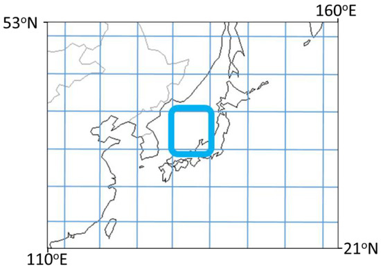
Figure 1.
The target grid (thick blue box) at 135.0° east (E) and 36.0° north (N) in the grid system (thin blue lines) within the Loch-Vecode-Ecbilt-Clio-agism (LOVECLIM) model.
2.3. Analysis Method
We analyzed the annual maximum monthly precipitation instead of the annual maximum daily precipitation because the temporal resolution of LOVECLIM allows resolving monthly or longer time scales according to the Orlanski observation scale of meteorological processes [16].
According to a conventional procedure for extreme value analysis, we first extracted the annual maximum monthly precipitation from the historical simulation time series, and then divided the 11,700 samples into 117 intervals consisting of 100 samples each. There are many parametric extreme value distributions which exist (e.g., [17]). For simplicity, we assumed a two-parameter Gumbel distribution [18] (because the Gumbel distribution is theoretically obtained under a stationary assumption) to estimate extreme precipitation for a given return level:
where F is the cumulative distribution function of the Gumbel distribution, xi represents an annual maximum monthly precipitation in interval i, and μi and βi represent location and scale of x. The L-moment method [19] was used to estimate the population parameter, and precipitation within the return level was estimated for each of the 117 samples.
Autocorrelation analysis was performed to determine the persistence of estimated annual maximum monthly precipitation within a certain return level over time. Bartlett’s test was used to determine the significance of autocorrelation.
We applied wavelets analysis to detect short-lived waves within a certain interval and frequency, whereas we used Fourier analysis to detect long-lived waves across the entire Holocene Period. Wavelet analysis is widely used in the field of Earth sciences (e.g., [20,21]). It allows expressing data as a combination of the scale and translation of a basic single-wavelength wave (mother wavelet). In Fourier analysis, only the wavenumber spatial information is extracted; however, in wavelet analysis, the spatiotemporal information can also be retained.
2.4. Data
Reconstructed Greenland average temperatures [14] were used to validate the time series of temperatures simulated using LOVECLIM for the entire Holocene period.
Precipitation at Maizuru (135.32° E, 35.45° N) was used for a comparison of present-day climatological mean monthly precipitation between the ground observation (available from http://hydro.iis.u-tokyo.ac.jp/CGLB [22]) and LOVECLIM. The intervals used were 1981–2010 for the ground observation and the last 30 years for the LOVECLIM simulation.
3. Current Climate Reproducibility
LOVECLIM has been used in numerous studies, especially paleoclimate studies that require long-term integration (e.g., [11,12,13,14]). Figure 2 depicts a time series of the surface air temperatures of reconstructed observations and LOVECLIM simulations for the Holocene. The surface air temperatures in LOVECLIM simulations were well reproduced in both Greenland (Figure 2a) and the Northern Hemisphere (Figure 2b) with respect to the reconstructed observations. LOVECLIM successfully reproduced the current climatology of zonal mean precipitation except for an overestimation in the subtropical region and a symmetric zonal distribution between the Northern and Southern Hemispheres (see Figure 11 in [13]). River discharges were adequately estimated with LOVECLIM with respect to the Holocene palaeohydrological records after statistical downscaling, including bias corrections for surface air temperatures and precipitation (see Figure 4 in [12]). These previous studies demonstrated a good reproducibility of the current climatology of precipitation on a global scale.
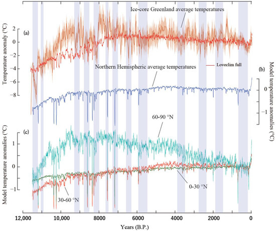
Figure 2.
(a) Time series of temperature anomalies reconstructed from a proxy of ice cores and of those simulated with LOVECLIM in Greenland during the Holocene. Thick and thin orange lines denote reconstructed and LOVECLIM results, respectively. (b) Time series of mean temperature anomalies in the Northern Hemisphere simulated with LOVECLIM. (c) Same as in (b) but represented separately for high (60–90° N) and mid (30–60° N), and low latitudes (0–30° N). An anomaly was defined as a deviation from the latest 1000 year mean temperatures. The light-blue shading denotes predominant climatic events. This figure was drawn on the basis of Figure 3 in [14] (CC BY).
Figure 2c depicts the zonal mean surface air temperatures for the mid-latitude region where the target grid was located. The surface air temperatures showed a monotonic increase during the Holocene with some climate variabilities such as the Medieval Warm Period. LOVECLIM successfully simulated annual precipitation with a 4% overestimation with respect to the observations. Both observed and simulated precipitation data in the target grid for the latest 30-year record presented two peaks in the winter and summer (Figure 3), whereas the third peak in July was not simulated with LOVECLIM. These seasonal changes in precipitation were seen in the Sea of Japan. Tropical cyclone-induced precipitation has a minor effect on monthly precipitation because it contributes to annual precipitation by about 2% [23]. Plausible reasons for this may include the difference in the Earth’s surface conditions between the observation station on coastal land and the target grid at sea, as well as the difference in the representative horizontal scale between the observation station and target grid. This obtained reproducibility allowed further analysis of extreme values.
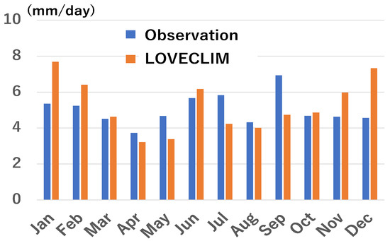
Figure 3.
Comparison of climatological mean precipitation between observation at Maizuru (135.32° E, 35.45° N) and LOVECLIM simulation.
4. Results and Discussion
4.1. 100-Year Climatological Annual Maximum Monthly Precipitation
Figure 4a shows the time series of the climatological mean of the annual maximum monthly precipitation for each 100-year interval. The range of fluctuation was relatively small with approximately 8.8–9.6 mm·day−1, equivalent to 24 mm·month−1. Therefore, the 100-year climatological mean of the annual maximum monthly precipitation did not change much in the target grid.
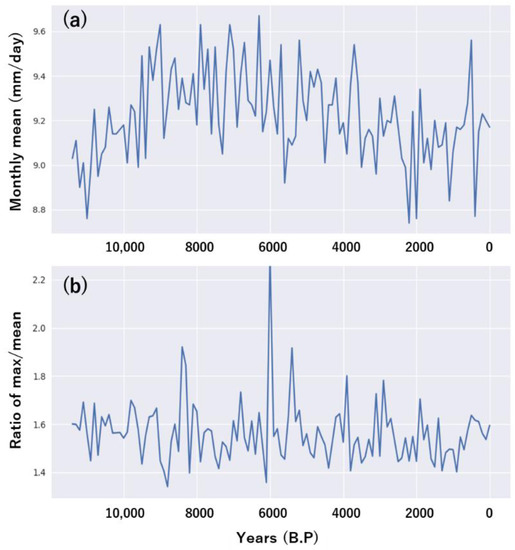
Figure 4.
(a) Time series of 100-year climatological mean of the annual maximum monthly precipitation in the Holocene simulated with LOVECLIM. (b) Same as in (a) but the ratio of the 100 year maximum of the annual maximum monthly precipitation to the 100-year climatological mean.
From the Holocene perspective, the 100-year climatological mean of the annual maximum monthly precipitation increased until 9000 BP, before varying greatly with a mean of 9.4 mm·day−1 until 5200 BP. Subsequently, the 100-year climatological mean decreased until 2000 BP. Following large variations around 2000 BP, the 100-year climatological mean remained at 9. 1 mm·day−1 until present, albeit with unprecedented large variations. The variations on a 10,000-year time scale probably correspond to the retreat of polar ice sheets, whereby the climatological zonal mean air temperature decreased after 9500 BP in the high-latitude region but not in the mid-latitude region (Figure 2c).
The 100-year maximum values of annual maximum monthly precipitation every 100 years are depicted as a time series after normalization in Figure 4b, with the climatological means for each 100-year period. These ratios had a mean value of about 1.5 with a relatively large range of 1.4–2.2 with respect to the 100-year climatological means in Figure 4a, with no obvious trend seen on the 10,000-year time scale. The maximum value of 2.3 occurred in the 100-year interval of 6000 BP (6100 BP to 6000 BP), followed by the second largest value of 1.93 in the 100-year interval of 8400 BP and the third largest value of 1.91 in the 100-year interval of 5500 BP. These peaks were not maintained for multiple 100-year intervals.
These abrupt occurrences of peaks prohibited us from proposing explanatory trends for the 100-year maximum of annual maximum monthly precipitation with respect to the 100-year climatological means. These results depict the aforementioned nonstationarity in support of our analysis which took 100 samples for each of the 100-year periods.
4.2. Estimated Annual Maximum Monthly Precipitation with a Return Level of 100 Years
Assuming stationarity of the annual maximum monthly precipitation for a given 100-year interval and the 100 samples distributed with a Gumbel distribution, we calculated the estimated annual maximum monthly precipitation with a return level of 100 years for each 100-year interval. The histogram of estimated annual maximum monthly precipitation in Figure 5a displays a distribution almost symmetric to the mode, although both tails seem less frequent. The red line denotes a normal distribution estimated on the basis of the histogram sample statistics. Over- and underestimations can be seen in the tails, whereas the estimated normal distribution fit the histogram, especially within ±1 σ. The low level of frequency exceeding ±2 σ confirmed the suitability of the estimated normal distribution. Large gaps at ±1 σ (22 and 24.5 mm·day−1) can be seen in Figure 5b. The skewness and kurtosis values of the data distribution were 0.05 and −0.19, representing a near-normal distribution. Moreover, Bartlett’s test was performed to detect the deviation from normality, further confirming the normal distribution (p < 0.01).
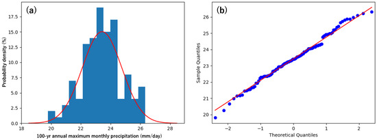
Figure 5.
(a) Histogram and (b) quantile–quantile map of the estimated annual maximum monthly precipitation with a return level of 100 years for each 100-year interval for the Holocene under the assumption of a Gumbel distribution. Red lines denote the normal distribution estimated on the basis of the histogram statistics.
4.3. Autocorrelation
Persistency was analyzed through an autocorrelation of the time series of estimated annual maximum monthly precipitation with a return level of 100 years for each 100-year interval. Note that the adjacent values were independently estimated from a set of 100 samples of a 100-year interval, whereby lag 1 denotes one 100-year interval. The estimated annual maximum monthly precipitation with a return level of 100 years for each 100-year interval was uncorrelated, even with lag 1 (Figure 6). In other words, the estimated annual maximum monthly precipitation within a 100-year interval was not related to the previous and subsequent intervals. Statistically significant periodicity with a lag of 25 or 2500 years was seen; however, this could not be attributed to a climatic phenomenon since no periodic climatic cycle with this lag is currently known.
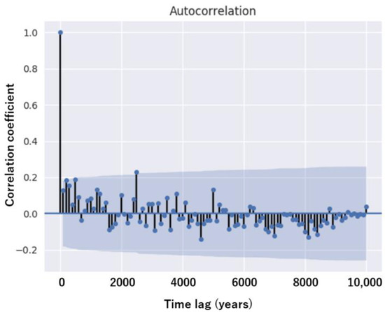
Figure 6.
Autocorrelation of the time series of the estimated annual maximum monthly precipitation with a return level of 100 years for each 100-year interval for the Holocene. The light-blue shading represents the significance interval at a 95% confidence level.
4.4. Wavelet Analysis
The time series of the annual maximum monthly precipitation with a return level of 100 years (black line) and that of the data inversely transformed using wavelet analysis (gray line) are depicted in Figure 7a. Both time series correlated well with the exception of three epochs: 8600 BP to 7900 BP, around 4000 BP, and 2000 BP to present. Therefore, the wavelet analysis with a Morlet function worked well.
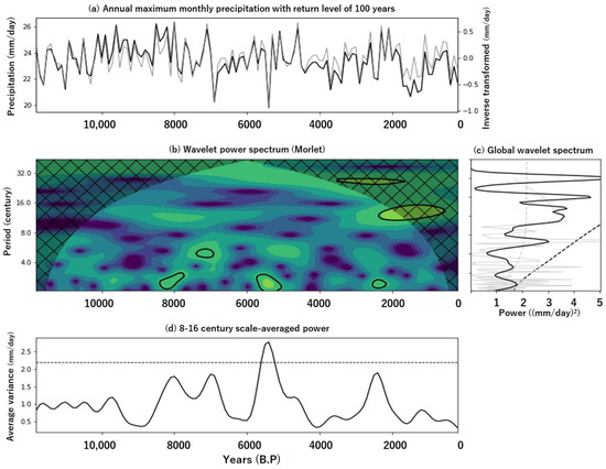
Figure 7.
Wavelet analysis of time series of the estimated annual maximum monthly precipitation with a return level of 100 years. The Morlet function was used as the other wavelet. (a) Time series of the original estimated annual maximum monthly precipitation with a return level of 100 years (black line) and the inverse transformed values (gray) from wavelet analysis. (b) Wavelet power spectrum. (c) Global wavelet spectrum (black) with a confidence level of 95% (black broken line). The gray solid line denotes the red noise power spectrum, while the gray dotted line denotes the 95% confidence level. (d) Average power scaled every 8–16 centuries. The horizontal broken line denotes the 95% confidence level.
Figure 7b shows the wavelet power spectrum of the annual maximum monthly precipitation with a return level of 100 years. The significant power spectrum indicated by the black line appeared only in a very limited area of the time–frequency space in Figure 7b. Here, 200-year cycles were found around 8000 BP, 5500 BP, and 2400 BP, while a 600-year cycle was found around 7200 BP. A long cycle of approximately 1200 years was found around 2000 BP to present. Significant powers could only be seen within such short epochs; however, the climate change leading to these powers requires further investigation. The local maxima of the power spectrum were, thus, very limited in the time–frequency space, while the local minima were widely distributed (e.g., 10,000–8000 BP at 300–800-year periods).
The global power spectrum (black line) is the sum of the magnitudes of the power spectrum for each frequency with respect to time or year, where almost the same result as the Fourier analysis can theoretically be obtained (Figure 7c). The global power spectrum had no significant signal with respect to the 95% confidence level (black dashed line). This corresponds to a significant power spectrum locally confined in the time frame, as seen in Figure 7b. On the other hand, the periods exceeding the power spectrum of red noise (gray dashed line) consisted of 200 years or approximately 1200 years, among others (see Figure 7b). Peaks were also seen with periods of approximately 1600 and 3200 years; however, these were only found in the Wavelet analysis due to the longer periods.
The power spectrum averaged over the band path filter with periods of 800–1600 years reached its maximum (about 2.4 mm·day−1) in 5200 BP with significance at a 95% confidence level only observed before and after 5200 BP (Figure 7d). This corresponds to the minimum of the estimated annual maximum monthly precipitation with a return level of 100 years in Figure 7a. The other local maxima of the average power spectrum in 7800 BP, 6800 BP, and 2200 BP occurred when the estimated annual maximum monthly precipitation with a return level of 100 years exhibited fluctuation with respect to local values. These fluctuations increased the amplitude and, thus, the average power spectrum.
5. Conclusions
We investigated the characteristics of extreme value statistics of the annual maximum monthly precipitation by simulating climate change on a time scale of thousands to tens of thousands of years over the past 12,000 years (i.e., the Holocene) with LOVECLIM providing a nonstationary time series of data in order to directly consider nonstationarity in the extreme value analysis instead of proxy data. We focused on a target grid in East Asia and performed extreme value analysis to obtain the estimated annual maximum monthly precipitation with a return level of 100 years. Despite numerous known climate events occurring in the past 12,000 years, such as the Medieval Warm Period and the Little Ice Age, there were no significant changes in estimated annual maximum monthly precipitation with a return level of 100 years. The climatological means of the annual maximum monthly precipitation for each 100-year interval displayed a nonstationary time series, while the ratios of the largest annual maximum monthly precipitation to the climatological mean displayed a nonstationary time series with large spike variations. The extreme value analysis revealed that the annual maximum monthly precipitation with a return level of 100 years estimated for each 100-year interval also presented a nonstationary time series which was normally distributed and not autocorrelated, even with the preceding and following 100-year interval (lag 1). Wavelet analysis of this time series showed that significant periodicity was detected only in confined areas of the time–frequency space. Therefore, the annual maximum monthly precipitation with a return level of 100 years simulated using an Earth system model of medium complexity showed nonstationary features for the entire Holocene Period. This first attempt to reveal the characteristics of extreme value analysis of the annual maximum monthly precipitation in the Holocene Period will hopefully motivate further studies on extreme value analysis of climate simulations incorporating the entire Holocene time scale, addressing not only stationarity in extreme value analysis in climate science, but also how to treat nonstationary time series.
This study focused on a grid point in East Asia to deepen our understanding of the characteristics of extreme values in the Holocene Period using LOVECLIM. This was done in an attempt to evaluate how the characteristics in the tropics and high-latitude regions are correlated to extreme values in East Asia. Future studies should reveal the differences and similarities among global-scale regions. Moreover, we would like to extend this extreme value analysis using different variables with different return levels and elucidate the physical factors such as volcanic activity and other external forcing factors, which produce nonstationary variabilities. Moreover, an Earth system model of comprehensive complexity may be an option to simulate the climates over the past 12,000 years in order to obtain more reliable extreme value statistics, although the available length of the time series may decrease by 10% or approximately 1000 years.
Author Contributions
Conceptualization and methodology, T.N.; simulations, T.K.; reproducibility, T.N.; formal analysis, H.K.; investigation, T.N., T.K., and H.K.; writing—original draft preparation, T.N.; writing—review and editing, T.K. and H.K.; visualization, supervision, project administration, and funding acquisition, T.N. All authors have read and agreed to the published version of the manuscript.
Funding
This research was funded by the Japan Society for the Promotion of Science, grant numbers 16H06291 and 20K12154, and by the Ministry of Education, Culture, Sports, Science, and Technology, Japan, Area Theme C: Integrated Climate Change Projection in Study Program for Greater Sophistication of Integrated Climate Model.
Acknowledgments
This study is carried out under a five-year project entitled “Research on Application of Weather Forecast Information to Disaster Prevention, Traffic and Industry” and “Research on Attribution and Projection of Climatic/Global Environmental Change” in the Meteorological Research Institute. We would like to acknowledge the constructive comments by three reviewers that improved the first version of this manuscript.
Conflicts of Interest
The authors declare no conflict of interest.
References
- Mukherjee, S.; Aadhar, S.; Stone, D.; Mishra, V. Increase in extreme precipitation events under anthropogenic warming in India. Weather Clim. Extrem. 2018, 20, 45–53. [Google Scholar] [CrossRef]
- Kawase, H.; Tsuguti, H.; Nakaegawa, T.; Seino, N.; Murata, A.; Takayabu, I. The Heavy Rain Event of July 2018 in Japan Enhanced by Historical Warming. Bull. Atmos. Meteorol. Soc. 2019, 101. [Google Scholar] [CrossRef]
- Koutsoyiannis, D. Statistics of extremes and estimation of extreme rainfall: II. Empirical investigation of long rainfall records. Hydrol. Sci. J. 2004, 49, 591–610. [Google Scholar] [CrossRef]
- Takara, K. Frequency Analysis of Larger Samples of Hydrologic Extreme-Value Data: How to estimate the T-year quantile for samples with a size of more than the return period T. Disaster Prev. Res. Inst. Annu. 2006, 49B, 7–12. [Google Scholar]
- Ishihara, K.; Nakaegawa, T. Estimation of Probable Daily Precipitation with Nonparametric Method at 51 Meteorological Observatories in Japan. J. Jpn. Soc. Hydrol. Wat. Resour. 2008, 21, 459–463. [Google Scholar] [CrossRef][Green Version]
- Nakaegawa, T. Estimation of the frequency analysis of annual maximum monthly precipitation in east Asia based on a dynamical ensemble method. Proc. Hydraul. Eng. 2004, 51, 295–300. [Google Scholar] [CrossRef]
- Nakaegawa, T. Characteristics of the Largest Recorded Annual Maximum Monthly Precipitation in an Atmospheric Global Climate Model Experiment. J. Jpn. Soc. Hydrol. Wat. Resour. 2010, 23, 373–383. [Google Scholar] [CrossRef]
- Mizuta, R.; Murata, A.; Ishii, M.; Shiogama, H.; Hibino, K.; Mori, N.; Arakawa, O.; Imada, Y.; Yoshida, K.; Aoyagi, T.; et al. Over 5000 years of ensemble future climate simulations by 60 km global and 20 km regional atmospheric models. Bull. Am. Meteor. Soc. 2017, 99, 1383–1398. [Google Scholar] [CrossRef]
- Sugi, M.; Imada, Y.; Nakaegawa, T.; Kamiguchi, K. Estimating probability of extreme rainfall over Japan using Extended Regional Frequency Analysis. Hydrol. Res. Lett. 2017, 11, 19–23. [Google Scholar] [CrossRef][Green Version]
- Cheng, L.; AghaKouchak, A.; Gilleland, E.; Katz, R.W. Non-stationary extreme value analysis in a changing climate. Clim. Chang. 2014, 127, 353–369. [Google Scholar] [CrossRef]
- Goosse, H.; Brovkin, V.; Fichefet, T.; Haarsma, R.; Huybrechts, P.; Jongma, J.; Mouchet, A.; Selten, F.; Barriat, P.Y.; Campin, J.M.; et al. Description of the Earth system model of intermediate complexity LOVECLIM version 1.2. Geosci. Model. Dev. 2010, 3, 603–633. [Google Scholar] [CrossRef]
- Ward, P.J.; Aerts, J.C.; de Moel, H.; Renssen, H. Verification of a coupled climate-hydrological model against Holocene palaeohydrological records. Glob. Planet. Chang. 2007, 57, 283–300. [Google Scholar] [CrossRef]
- Ward, P.J.; Renssen, H.; Aerts, J.C.; Verburg, P.H. Sensitivity of discharge and flood frequency to twenty-first century and late Holocene changes in climate and land use (River Meuse, northwest Europe). Clim. Chang. 2011, 106, 179–202. [Google Scholar] [CrossRef]
- Kobashi, T.; Menviel, L.; Jeltsch-Thömmes, A.; Vinther, B.M.; Box, J.E.; Muscheler, R.; Nakaegawa, T.; Pfister, P.L.; Döring, M.; Leuenberger, M.; et al. Volcanic influence on centennial to millennial Holocene Greenland temperature change. Sci. Rep. 2017, 7. [Google Scholar] [CrossRef]
- Stuhne, G.R.; Peltier, W.R. Reconciling the ICE-6G_C reconstruction of glacial chronology with ice sheet dynamics: The cases of Greenland and Antarctica. J. Geophys. Res. Earth Surf. 2015, 120, 1–25. [Google Scholar] [CrossRef]
- Orlanski, I. A rational subdivision of scales for atmospheric processes. Bull. Am. Meteorol. Soc. 1975, 56, 527–530. [Google Scholar]
- Molina-Aguilar, J.P.; Gutierrez-Lopez, A.; Raynal-Villaseñor, J.A.; Garcia-Valenzuela, L.G. Optimization of Parameters in the Generalized Extreme-Value Distribution Type 1 for Three Populations Using Harmonic Search. Atmosphere 2019, 10, 257. [Google Scholar] [CrossRef]
- Młyński, D.; Wałęga, A.; Petroselli, A.; Tauro, F.; Cebulska, M. Estimating Maximum Daily Precipitation in the Upper Vistula Basin, Poland. Atmosphere 2019, 10, 43. [Google Scholar] [CrossRef]
- Hosking, J.R.M. L-moments: Analysis and estimation of distributions using linear combinations of order statistics. J. R. Stat. Soc. Ser. B 1990, 52, 105–124. [Google Scholar] [CrossRef]
- Nakaegawa, T. Preliminary study of the relationship between precipitation over japan and Niño 3 sea surface temperature. Proc. Hydraul. Eng. 2004, 48, 85–90. [Google Scholar] [CrossRef][Green Version]
- Kobashi, T.; Severinghaus, J.P.; Barnola, J.M.; Kawamura, K.; Carter, T.; Nakaegawa, T. Persistent multi-decadal Greenland temperature fluctuation through the last millennium. Clim. Chang. 2010, 100, 733–756. [Google Scholar] [CrossRef]
- Nakaegawa, T.; Horiuchi, S.; Kim, H. Development of a web application for examining climate data of global lake basins: CGLB. Hydrol. Res. Lett. 2015, 9, 125–132. [Google Scholar] [CrossRef]
- Kamahori, H.; Arakawa, O. Tropical cyclone induced precipitation over Japan using observational data. SOLA 2018, 14, 165–169. [Google Scholar] [CrossRef]


Publisher’s Note: MDPI stays neutral with regard to jurisdictional claims in published maps and institutional affiliations. |
© 2020 by the authors. Licensee MDPI, Basel, Switzerland. This article is an open access article distributed under the terms and conditions of the Creative Commons Attribution (CC BY) license (http://creativecommons.org/licenses/by/4.0/).