The Use of a Physiologically Based Pharmacokinetic Modelling in a “Full-Chain” Exposure Assessment Framework: A Case Study on Urban and Industrial Pollution in Northern Italy


Abstract
:1. Introduction
2. Methods
2.1. HBM Study
2.2. Exposure Assessment
2.3. Air Route
2.4. Indoor/Outdoor Coefficient
2.5. Chemical Speciation
2.6. Diet Route
2.7. Use of MERLIN-Expo
2.8. PBPK Model Parametrization
3. Results
3.1. Comparison between the MERLIN Platform and the HBM Study Results
3.2. Exposed vs. Non-Exposed
3.3. Concentration in Urine
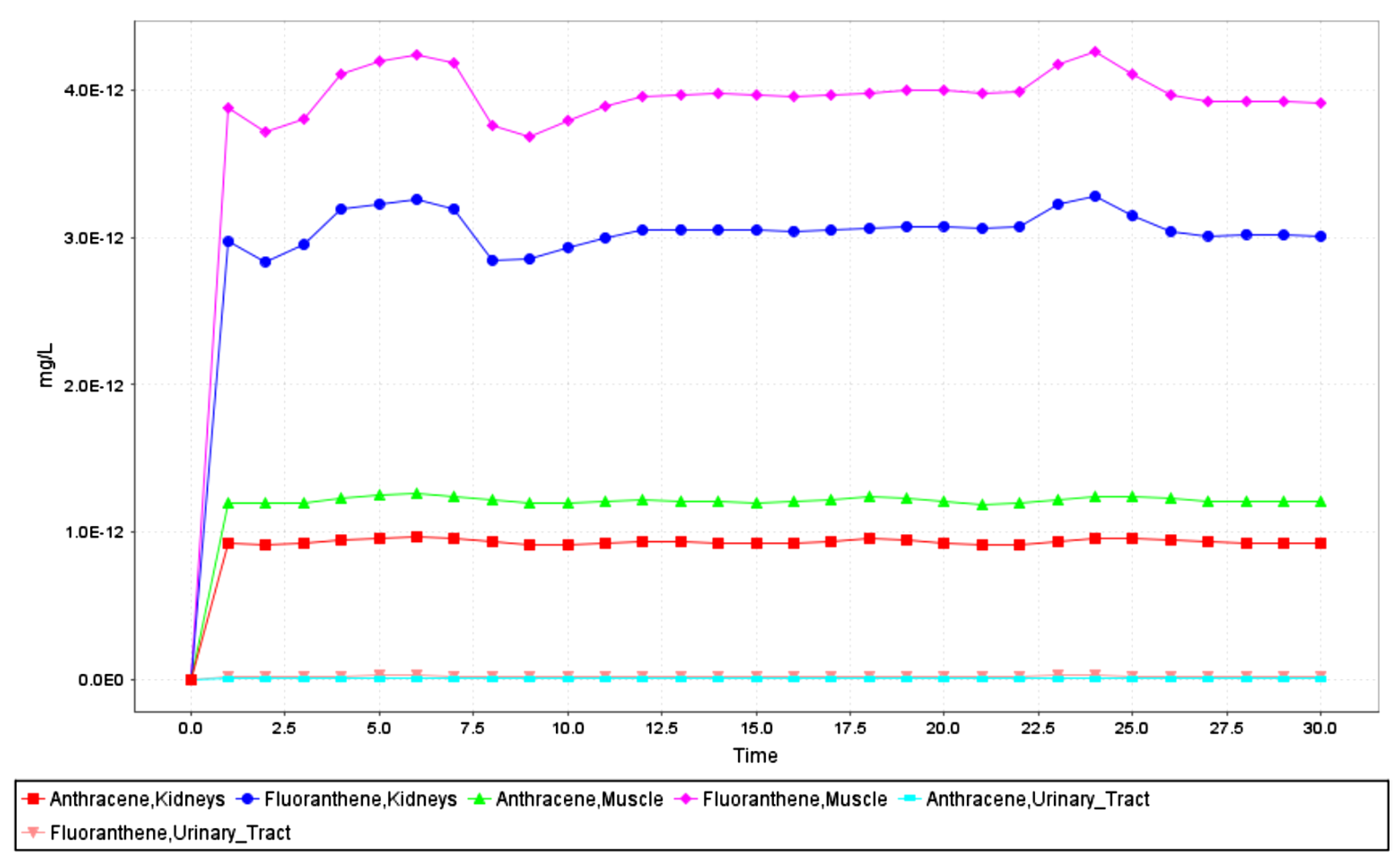
3.4. Concentration in Organs and Tissues
3.5. Distance Analysis
4. Discussion
4.1. Comparison between MERLIN Software and HBM Study Results
4.2. Exposed vs. Non-Exposed
4.3. Diet Scenario
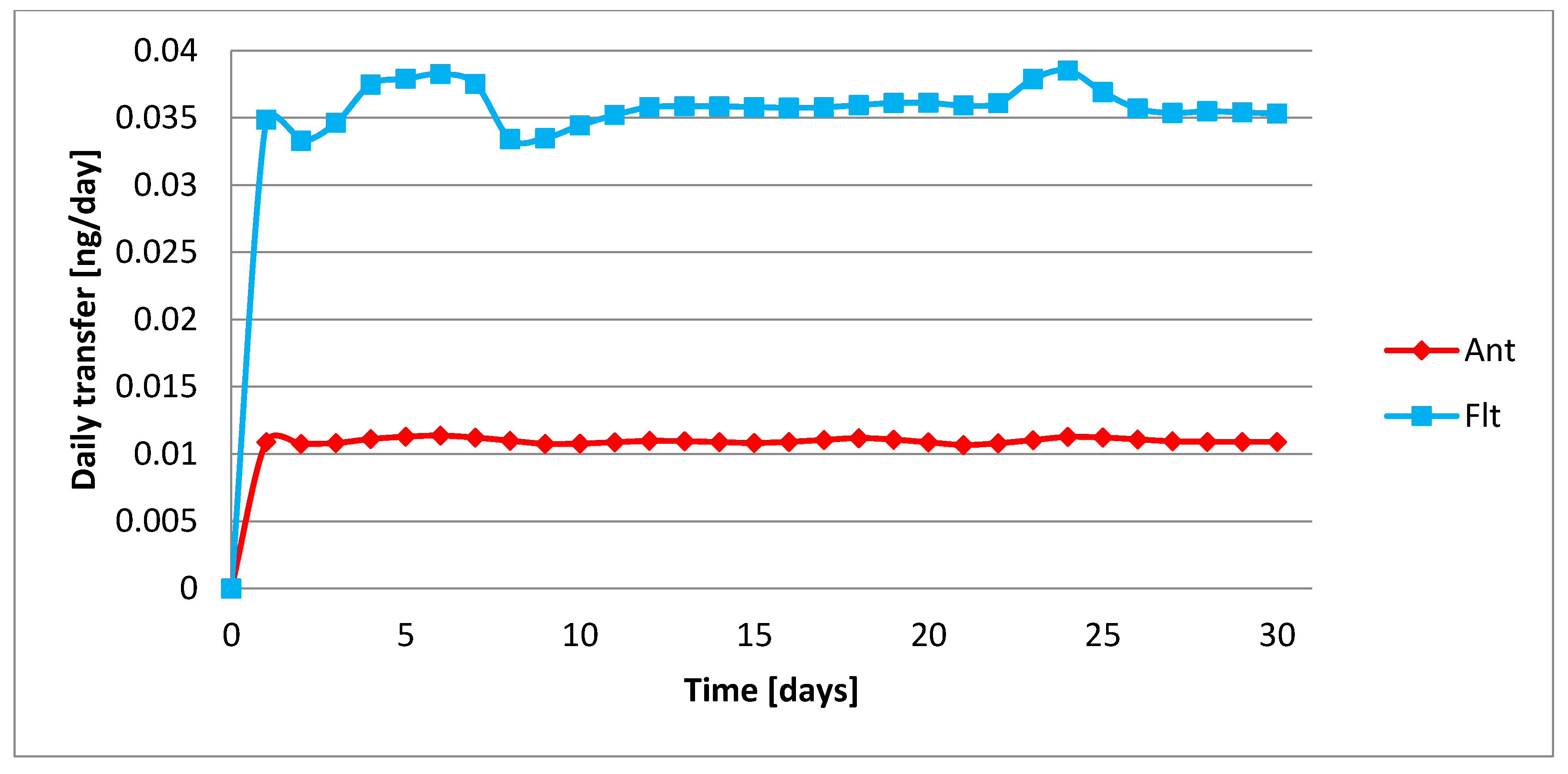
4.4. Mass Balance
5. Conclusions
Author Contributions
Funding
Conflicts of Interest
References
- U.S. EPA (U.S. Environmental Protection Agency). Guidelines for Human Exposure Assessment; (EPA/100/B-19/001); Risk Assessment Forum; U.S. EPA: Washington, DC, USA, 2019.
- Merlin-Expo. 2016. Available online: http://merlin-expo.eu (accessed on 10 October 2018).
- Ciffroy, P.; Alfonso, B.; Altenpohl, A.; Banjac, Z.; Bierkens, J.; Brochot, C.; Critto, A.; De Wilde, T.; Fait, G.; Fierens, T.; et al. Modelling the exposure to chemicals for risk assessment: A comprehensive library of multimedia and PBPK models for integration, prediction, uncertainty and sensitivity analysis—The MERLIN-Expo tool. Sci. Total Environ. 2016, 568, 770–784. [Google Scholar] [CrossRef] [PubMed]
- Fierens, T.; Van Holderbeke, M.; Standaert, A.; Cornelis, C.; Brochot, C.; Ciffroy, P.; Johansson, E.; Bierkens, J. Multimedia & PBPK modelling with MERLIN-Expo versus biomonitoring for assessing Pb exposure of pre-school children in a residential setting. Sci. Total Environ. 2016, 568, 785–793. [Google Scholar] [PubMed]
- Ciffroy, P.; Tanaka, T.; Johansson, E.; Brochot, C. Linking fate model in freshwater and PBPK model to assess human internal dosimetry of B(a)P associated with drinking water. Environ. Geochem. Health 2011, 33, 371–387. [Google Scholar] [CrossRef] [PubMed]
- Fàbrega, F.; Kumar, V.; Schuhmacher, M.; Domingo, J.L.; Nadal, M. PBPK modelling for PFOS and PFOA: Validation with human experimental data. Toxicol. Lett. 2014, 230, 244–251. [Google Scholar] [CrossRef] [PubMed]
- AEIFORIA. 4FUN Project (case study 1). In The FUture of FUlly Integrated Human Exposure Assessment of Chemicals: Ensuring the Long-Term Viability and Technology Transfer of the EU-FUNded 2-FUN Tools as Standardised Solution; Deliverable D5.1: Report on Case Study 1; AEIFORIA: Noida, India, 2015. [Google Scholar]
- AEIFORIA. 4FUN Project (case study 2). In The FUture of FUlly Integrated Human Exposure Assessment of Chemicals: Ensuring the Long-Term Viability and Technology Transfer of the EU-FUNded 2-FUN Tools as Standardised Solution; Deliverable D5.2: Report on Case Study 2; AEIFORIA: Noida, India, 2015. [Google Scholar]
- AEIFORIA. 4FUN Project (case study 3). In The FUture of FUlly Integrated Human Exposure Assessment of Chemicals: Ensuring the Long-Term Viability and Technology Transfer of the EU-FUNded 2-FUN Tools as Standardised Solution; Deliverable D5.3: Report on case study 3; AEIFORIA: Noida, India, 2015. [Google Scholar]
- Van Teijlingen, E.R.; Hundley, V. The Importance of Pilot Studies; Social Research Update; University of Aberdeen: Aberdeen, UK, 2001. [Google Scholar]
- Suciu, N.A.; Capri, E.; Trevisan, M.; Tanaka, T.; Tien, H.; Heise, S.; Schuhmacher, M.; Nadal, M.; Rovira, J.; Seguí, X.; et al. Human and Environmental Impact Produced by E-Waste Releases at Guiyu Region (China). Handb. Environ. Chem. 2012, 23, 349–384. [Google Scholar]
- Ranzi, A.; Fustinoni, S.; Erspamer, L.; Campo, L.; Gatti, M.G.; Bechtold, P.; Bonassi, S.; Trenti, T.; Goldoni, C.A.; Bertazzi, P.A.; et al. Biomonitoring of the general population living near a modern solid waste incinerator: A pilot study in Modena, Italy. Environ. Int. 2013, 61, 88–97. [Google Scholar] [CrossRef] [PubMed]
- Marchei, E.; Pellegrini, M.; Pacifici, R.; Zuccaro, P.; Pichini, S. Composizione Chimica del Fumo Principale di Sigaretta; Istituto Superiore di Sanità, Dipartimento del farmaco: Rome, Italy, 2003. [Google Scholar]
- Gandini, M.; Berti, G.; Cattani, G.; Scarinzi, C.; De’Donato, F.; Accetta, G.; Angiuli, L.; Caldara, S.; Carreras, G.; Casale, P.; et al. Environmental indicators in EpiAir2 project: Air quality data for epidemiological surveillance. Epidemiol. Prev. 2013, 37, 209–219. (In Italian) [Google Scholar] [PubMed]
- Sajani, S.Z.; Ricciardelli, I.; Trentini, A.; Bacco, D.; Maccone, C.; Castellazzi, S.; Lauriola, P.; Poluzzi, V.; Harrison, R.M. Spatial and indoor/outdoor gradients in urban concentrations of ultrafine particles and PM2.5 mass and chemical components. Atmos. Environ. 2015, 103, 307–320. [Google Scholar] [CrossRef]
- Urso, P.; Cattaneo, A.; Garramone, G.; Peruzzo, C.; Cavallo, D.M.; Carrer, P. Identification of particulate matter determinants in residential home. Build. Environ. 2015, 86, 61–69. [Google Scholar] [CrossRef]
- Mandin, C.; Trantallidi, M.; Cattaneo, A.; Canha, N.; Mihucz, V.G.; Szigeti, T.; Mabilia, R.; Perreca, E.; Spinazzè, A.; Fossati, S.; et al. Assessment of indoor air quality in office buildings across Europe—The OFFICAIR study. Sci. Total Environ. 2016, 579, 169–178. [Google Scholar] [CrossRef] [PubMed] [Green Version]
- Cattaneo, A.; Peruzzo, C.; Garramone, G.; Urso, P.; Ruggeri, R.; Carrer, P.; Cavallo, D.M. Airborne particulate matter and gaseous air pollutants in residential structures in Lodi province, Italy. Indoor Air 2011, 21, 489–500. [Google Scholar] [CrossRef] [PubMed]
- Meier, R.; Eeftens, M.; Phuleria, H.C.; Ineichen, A.; Corradi, E.; Davey, M.; Fierz, M.; Ducret-Stich, R.E.; Aguilera, I.; Schindler, C.; et al. Differences in indoor versus outdoor concentrations of ultrafine particles, PM2.5, PMabsorbance and NO2 in Swiss homes. J. Expo. Sci. Environ. Epidemiol. 2015, 25, 499–505. [Google Scholar] [CrossRef] [PubMed]
- Regione Emilia-Romagna. I Risultati del Progetto Moniter. Gli Effetti Dell’Inceneritore Sull’Ambiente e la Salute in Emilia-Romagna. ARPA Emilia-Romagna. Quaderni progetto MONITER. 2011. Available online: https://www.arpae.it/cms3/documenti/moniter/quaderni/04_Risultati_Moniter.pdf (accessed on 20 December 2018).
- Società Italiana di Nutrizione Umana. LARN: Livelli di Assunzione di Riferimento di Nutrienti ed Energia per la Popolazione Italiana, 4th ed.; SICS: Milan, Italy, 2014.
- Bocca, B.; Crebelli, R.; Menichini, E. Presenza degli Idrocarburi Policiclici Aromatici negli Alimenti; Rapporti ISTISAN: Rome, Italy, 2003. [Google Scholar]
- Reinik, M.; Tamme, T.; Roasto, M.; Juhkam, K.; Tenno, T.; Kiis, A. Polycyclic aromatic hydrocarbons (PAHs) in meat products and estimated PAH intake by children and general population in Estonia. Food Addit. Contam. 2007, 24, 429–437. [Google Scholar] [CrossRef]
- CCME (Canadian Council of Ministers of the Environment). Canadian Soil Quality Guidelines for Carcinogenic and Other Polycyclic Aromatic Hydrocarbons (Environmental and Human Health Effects); Scientific Criteria Document (revised); Canadian Council of Ministers of the Environment: Winnipeg, MB, Canada, 2010. [Google Scholar]
- Cicchella, D.; Hoogewerff, J.; Albanese, S.; Adamo, P.; Lima, A.; Taiani, M.V.E.; De Vivo, B. Distribution of toxic elements and transfer from the environment to humans traced by using lead isotopes. A case of study in the Sarno River basin, south Italy. Environ. Geochem. Health 2016, 38, 619–637. [Google Scholar] [CrossRef] [Green Version]
- Danieli, P.P.; Serrani, F.; Primi, R.; Ponzetta, M.P.; Ronchi, B.; Amici, A. Cadmium, Lead, and Chromium in Large Game: A Local-Scale Exposure Assessment for Hunters Consuming Meat and Liver of Wild Boar. Arch. Environ. Contam. Toxicol. 2012, 63, 612–627. [Google Scholar] [CrossRef] [Green Version]
- Larsen, J.C. Scientific Opinion of the Panel on Contaminants in the Food Chain on a request from the European Commission on Polycyclic Aromatic Hydrocarbons in Food. EFSA J. 2008, 724, 1–114. [Google Scholar]
- Gray, P.J.; Mindak, W.R.; Cheng, J. Inductively Coupled Plasma-Mass Spectrometric Determination of Arsenic, Cadmium, Chromium, Lead, Mercury, and Other Elements in Food Using Microwave Assisted Digestion; Elemental Analysis Manual for Food and Related Products; US Food and Drug Administration: Montgomery, MD, USA, 2015.
- Motorykin, O.; Santiago-Delgado, L.; Rohlman, D.; Schrlau, J.E.; Harper, B.; Harris, S.; Harding, A.; Kile, M.L.; Simonich, S.L.M. Metabolism and Excretion Rates of Parent and Hydroxy-PAHs in Urine Collected after Consumption of Traditionally Smoked Salmon for Native American Volunteers. Sci. Total Environ. 2015, 514, 170–177. [Google Scholar] [CrossRef] [PubMed] [Green Version]
- Sarigiannis, D.; Gotti, A.; Karakitsios, S. User Guide of the INTEGRA Computational Platform; Centre for Research and Technology Hellas (CERTH): Thessaloniki, Greece, 2017. [Google Scholar]
- Brochot, C. Documentation of the Models Implemented in 4FUN, the Human Model. 2016. Available online: https://merlin-expo.eu/learn/documentation/model-documentation (accessed on 10 October 2018).
- Arnaut, L.; Burrows, H. Chemical Kinetics-From Molecular Structure to Chimical Reactivity; Elsevier: Amsterdam, The Netherlands, 2007. [Google Scholar]
- Fesce, R.; Fumagalli, G. Farmacologia Generale e Molecolare, 4th ed.; UTET: Milan, Italy, 2016.
- David, L.; Michael, M. Iprincipi di Biochimica di Lehninger, 4th ed.; Zanichelli: Bologna, Italy, 2006. [Google Scholar]
- WHO (World Health Organization). Population health and waste management: Scientific data and policy options. In Proceedings of the Report of a WHO Workshop, Rome, Italy, 29–30 March 2007; Available online: http://www.euro.who.int/document/E91021.pdf (accessed on 13 May 2018).


| Group | p Value χ2 | Normal Distribution α = 0.05 | p Value | Homogeneity α = 0.05 | |
|---|---|---|---|---|---|
| Age | E | 0.23 | YES | 0.53 (T) | YES |
| NE | 0.73 | YES | |||
| Weight | E | 0.10 | YES | 0.20 (T) | YES |
| NE | 0.13 | YES | |||
| Height | E | 0.71 | YES | 0.03 (T) | NO |
| NE | 0.57 | YES | |||
| BMI | E | 0.02 | NO | 0.54 (K-S) | YES |
| NE | 0.01 | NO |
| Group | A.V. | St. Dev. | 95%CI | |
|---|---|---|---|---|
| Age | E | 48.3 | 5.6 | 45.8–50.8 |
| NE | 47.2 | 6.1 | 44.8–49.6 | |
| E + NE | 47.7 | 5.8 | 46.0–49.4 | |
| Weight | E | 73.9 | 13.4 | 67.7–80.0 |
| NE | 68.8 | 13.9 | 63.3–74.2 | |
| E + NE | 70.9 | 13.8 | 67.0–74.9 | |
| Height | E | 172 | 6.5 | 169–175 |
| NE | 167 | 9.2 | 164–171 | |
| E + NE | 1.69 | 8.44 | 1.67–1.72 |
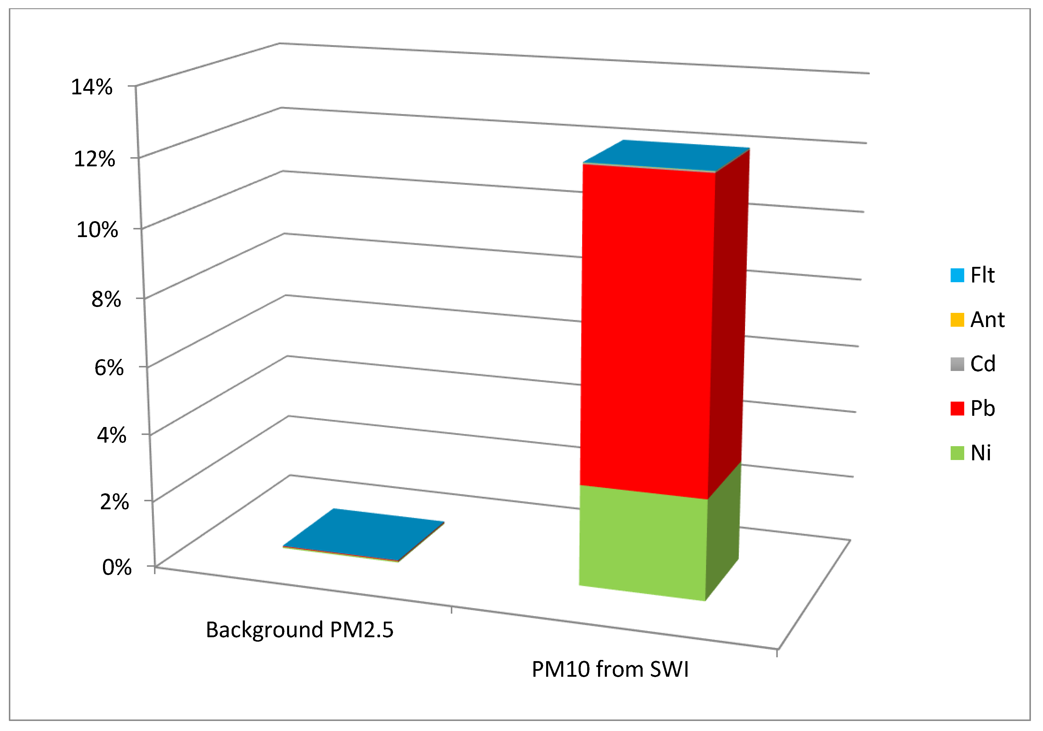
| PM | Ni | Pb | Cd | Ant | Flt |
|---|---|---|---|---|---|
| Background PM2.5 | 3.9 × 10⁻⁴ | 2.48 × 10⁻⁴ | 3 × 10⁻⁶ | 1.2 × 10⁻⁵ | 8.0 × 10⁻⁵ |
| PM10 from SWI | 3.02 × 10⁻² | 9.09 × 10⁻² | 3.65 × 10⁻⁴ | 1.04 × 10⁻⁴ | 1.04 × 10⁻⁴ |
| Type of Food | A.V. E | A.V. NE | St. Dev. E | St. Dev. NE |
|---|---|---|---|---|
| Meat | 3.9 | 3.6 | 3.2 | 2.1 |
| Grilled meat | 1.2 | 0.2 | 0.7 | 0.3 |
| Fish | 1.3 | 1.5 | 0.9 | 1.1 |
| Cheese | 4.6 | 3.3 | 2.3 | 2.0 |
| Egg | 1.3 | 1.4 | 0.7 | 1.4 |
| Fruit | 9.1 | 9.8 | 4.1 | 5.9 |
| Vegetable | 9.1 | 12.6 | 3.2 | 7.0 |
| Pasta | 12.1 | 10.0 | 6.2 | 5.6 |
| Mushroom | 0.7 | 0.3 | 0.9 | 0.3 |
| Wine | 6.7 | 2.6 | 9.5 | 3.6 |
| Milk | 6.3 | 4.0 | 4.5 | 3.4 |
| Type of Food | Pb (µg/kg) | Flt (WCS) (ng/kg) | Flt (MLS) (ng/kg) | Ant (WCS) (ng/kg) | Ant (MLS) (ng/kg) |
|---|---|---|---|---|---|
| Meat | 24.68 | 1.1 | 0.8 | 0.37 | 0.272 |
| Grilled meat | 27.00 | 102 | 20 | 34.68 | 6.8 |
| Fish | 17.31 | 1.9 | 0.6 | 0.65 | 0.204 |
| Cheese | 5.96 | 0.1 | 0.1 | 0.03 | 0.034 |
| Egg | 6.43 | 0.2 | 0.1 | 0.07 | 0.034 |
| Fruit | 16.79 | 3.6 | 1.2 | 1.22 | 0.408 |
| Vegetable | 17.98 | 117 | 19.4 | 39.78 | 6.6 |
| Pasta | 24.37 | 3.9 | 2.15 | 1.33 | 0.731 |
| Mushroom | 21.35 | 117 | 19.4 | 39.78 | 6.6 |
| Wine | 40.33 | 1.2 | 1.2 | 0.41 | 0.408 |
| Milk | 6.43 | 0.2 | 0.1 | 0.07 | 0.034 |
| Statistical Indices | Pb, Blood, M (µg/L) | Pb, Blood, HBM (µg/L) | Pb, Urine, M (µg/L) | Pb, Urine, HBM (µg/L) | Ant, Urine, M (ng/L) | Ant, Urine, HBM (ng/L) | Flt, Urine, M (ng/L) | Flt, Urine, HBM (ng/L) |
|---|---|---|---|---|---|---|---|---|
| A.V. | 7.98 × 10⁻⁴ | 2.52 | 0.41 | 0.40 | 0.02 | 0.54 | 0.06 | 2.17 |
| St. Dev. | 3.09 × 10⁻⁴ | 1.80 | 0.28 | 0.45 | 0.01 | 0.44 | 0.03 | 1.80 |
| Statistical Indices | Pb, Blood, M (µg/L) | Pb, Blood, HBM (µg/L) | Pb, Urine, M (µg/L) | Pb, Urine, HBM (µg/L) | Ant, Urine, M (ng/L) | Ant, Urine, HBM (ng/L) | Flt, Urine, M (ng/L) | Flt, Urine, HBM (ng/L) |
|---|---|---|---|---|---|---|---|---|
| A.V. | 9.1 × 10⁻⁴ | 3.09 | 0.45 | 0.46 | 0.02 | 0.76 | 0.05 | 2.40 |
| St. Dev. | 3.6 × 10⁻⁴ | 2.27 | 0.34 | 0.53 | 0.01 | 0.57 | 0.03 | 2.54 |
| Statistical Indices | Pb, Blood, M (µg/L) | Pb, Blood, HBM (µg/L) | Pb, Urine, M (µg/L) | Pb, Urine, HBM (µg/L) | Ant, Urine, M (ng/L) | Ant, Urine, HBM (ng/L) | Flt, Urine, M (ng/L) | Flt, Urine, HBM (ng/L) |
|---|---|---|---|---|---|---|---|---|
| A.V. | 7.2 × 10⁻⁴ | 2.10 | 0.39 | 0.35 | 0.02 | 0.37 | 0.06 | 2.00 |
| St. Dev. | 2.4 × 10⁻⁴ | 1.30 | 0.22 | 0.39 | 0.01 | 0.21 | 0.04 | 0.95 |
| Statistical Indices | Pb, Blood, E (µg/L) | Pb, Blood, NE (µg/L) | Pb, Urine, E (µg/L) | Pb, Urine, NE (µg/L) | Ant, E (ng/L) | Ant, NE (ng/L) | Flt, E (ng/L) | Flt, NE (ng/L) |
|---|---|---|---|---|---|---|---|---|
| A.V. | 2.1 × 10⁻⁵ | 1.0 × 10⁻⁵ | 0.007 | 0.010 | 0.001 | 0.001 | 0.007 | 0.005 |
| St. Dev. | 5.3 × 10⁻⁵ | 2.3 × 10⁻⁵ | 0.009 | 0.020 | 0.000 | 0.001 | 0.003 | 0.004 |
| Statistical Index | Pb, Urine | Pb, Blood | Ant | Flt |
|---|---|---|---|---|
| p value, K-S | 0.974 | 0.998 | 0.765 | 0.134 |
| Statistical indices | Pb, blood, E (µg/L) | Pb, Blood, NE (µg/L) | Pb, Urine, E (µg/L) | Pb, Urine, NE (µg/L) | Ant, E (ng/L) | Ant, NE (ng/L) | Flt, E (ng/L) | Flt, NE (ng/L) |
|---|---|---|---|---|---|---|---|---|
| M | 2.29 | 1.39 | 1.54 | 2.54 | 5.81 | 4.11 | 12.86 | 8.79 |
| (A.V.) | 1.84 | 2.04 | 4.96 | 10.83 | ||||
| HBM | 0.001 | 4.7 × 10⁻⁴ | 1.48 | 2.80 | 0.12 | 0.21 | 0.27 | 0.26 |
| (A.V.) | 0.001 | 2.14 | 0.17 | 0.27 | ||||
| Group | Pb, Blood | Pb, Urine | Ant | Flt |
|---|---|---|---|---|
| E | 97.71 | 98.46 | 94.19 | 87.14 |
| NE | 98.61 | 97.46 | 95.89 | 91.21 |
| A.V. | 98.16 | 97.96 | 95.04 | 89.17 |
| Group | Pb, Blood | Pb, Urine | Ant | Flt |
|---|---|---|---|---|
| E | 100.00 | 98.52 | 99.88 | 99.73 |
| NE | 100.00 | 97.20 | 99.79 | 99.74 |
| A.V. | 100.00 | 97.86 | 99.83 | 99.73 |
Publisher’s Note: MDPI stays neutral with regard to jurisdictional claims in published maps and institutional affiliations. |
© 2020 by the authors. Licensee MDPI, Basel, Switzerland. This article is an open access article distributed under the terms and conditions of the Creative Commons Attribution (CC BY) license (http://creativecommons.org/licenses/by/4.0/).
Share and Cite
Vaccari, L.; Ranzi, A.; Colacci, A.; Ghermandi, G.; Teggi, S. The Use of a Physiologically Based Pharmacokinetic Modelling in a “Full-Chain” Exposure Assessment Framework: A Case Study on Urban and Industrial Pollution in Northern Italy. Atmosphere 2020, 11, 1228. https://doi.org/10.3390/atmos11111228
Vaccari L, Ranzi A, Colacci A, Ghermandi G, Teggi S. The Use of a Physiologically Based Pharmacokinetic Modelling in a “Full-Chain” Exposure Assessment Framework: A Case Study on Urban and Industrial Pollution in Northern Italy. Atmosphere. 2020; 11(11):1228. https://doi.org/10.3390/atmos11111228
Chicago/Turabian StyleVaccari, Lorenzo, Andrea Ranzi, Annamaria Colacci, Grazia Ghermandi, and Sergio Teggi. 2020. "The Use of a Physiologically Based Pharmacokinetic Modelling in a “Full-Chain” Exposure Assessment Framework: A Case Study on Urban and Industrial Pollution in Northern Italy" Atmosphere 11, no. 11: 1228. https://doi.org/10.3390/atmos11111228
APA StyleVaccari, L., Ranzi, A., Colacci, A., Ghermandi, G., & Teggi, S. (2020). The Use of a Physiologically Based Pharmacokinetic Modelling in a “Full-Chain” Exposure Assessment Framework: A Case Study on Urban and Industrial Pollution in Northern Italy. Atmosphere, 11(11), 1228. https://doi.org/10.3390/atmos11111228