Meteorological Detrending of Ozone at Three Sites in the Dallas-Fort Worth Area: Application of KZ Filter Method

Abstract

The Dallas-Fort Worth (DFW) area that experiences high temperature and intense solar radiation falls into the moderate nonattainment classification. The variation in meteorological parameters plays an important role in ambient ozone levels variation. Meteorological influences need to be decoupled from ozone data for long-term trend analysis. Temporal separation of maximum daily average 8-h ozone (MDA8 ozone), maximum daily temperature (TMAX), daily average solar radiation (DASR), and daily average wind speed (DAWS) were conducted using Kolmogorov-Zurbenko (KZ) filter for ozone records at Keller (C17), Arlington (C61), Red Bird (C402) monitoring stations in the DFW area from 2003 to 2017. Temporal separation, regression analysis, and meteorological detrending were performed. The long-term component had a clear and stable trend. The contribution of the long-term component to total variation was negligible, which is less than 2%. This is due to the removal of the data noise from the original time series data. The seasonal component had a major contribution (55% to 72%) in the total variation of the maximum temperature and solar radiation. However, the short-term component was dominant in the total variation of the MDA8 ozone (41–54%) and wind speed (68–79%). Regression analysis showed the baseline component bears the highest correlation than the short-term and raw. Solar radiation had the highest correlation to the MDA8 ozone, followed by temperature data in all three stations. Meteorological detrending showed the detrended long-term ozone had an increasing trend. The increasing trend was significant at C402 with a trend of 0.19 ± 0.006 ppb/y (0.398 R²), whereas slight increasing trends were found at C17 (0.072 ± 0.006 (0.107 R²)) and at C61 (0.019 ± 0.007 (0.005 R²)). The increasing trend of long-term components of MDA8 ozone was justified by the increasing level of NO_x and VOCs from the mobile sources in the DFW area.

1. Introduction

Air pollution has significantly increased in the last 50 years, which poses a serious threat to human health. Over the years, the concern of pollutants (sulfur dioxide) emitted due to fossil fuel consumption has been shifted to new pollutants (Nitrogen Oxides (NOx), Volatile Organic Compounds (VOCs), and ozone due to the increased use of vehicles in urban areas [1]. Ozone is formed secondarily from the reaction between NO_x and VOCs in the presence of sunlight. As ozone formation occurs during day-time, mostly in summer, the ozone problems are more likely short-term and seasonal. Higher levels of ozone have been detected in the tropospheric layer of some large cities all over the world. A total of 196 counties in the U.S. are in the Non-Attainment Area List of USEPA according to the 8-H Ozone (2015) National Ambient Air Quality Standards (NAAQS) [2]. Due to the complex relation of ozone emissions and meteorological parameters, the ozone monitoring and control program has been a subject of the challenge for the managers and related agencies. The meteorological parameters always play an important role in the formation, transportation, and dispersion of air pollutions. Temperature, wind speed/direction, and solar radiation are some of the key parameters which have a significant influence on the air pollution mechanism [3,4,5]. Rao et al. (1997) suggested various levels of the effects due to time scales in the analysis of pollutant concentrations [6]. The pollutant concentration due to meteorological conditions has less impact due to a long term-trend than seasonal variations. The influence of meteorological factors on tropospheric ozone can be identified and analyzed using statistical modeling. Broadly, three statistical methods have been used (regression-based modeling, extreme value approaches, and space-time model) for the analysis of time-series data [7]. Each method has its advantages and disadvantages. Based on the characteristics and capability of the nature of data handling, a time series filtering model is useful for our long-time series data. The KZ filter time series model has been successfully used to evaluate the long-term trend of ozone and adjustment of meteorological parameters in the previous studies done by Rao and Zurbenko (1995), Milanchus et al. (1998), Wise and Comrie (2005), Hogrefe et al. (2000), Sa et al. (2015), and Ma et al. (2016) [8,9,10,11,12,13].

The KZ filter is a low pass filter that accounts for the moving average of time series data [8]. Kolmogorov introduced this filter in his study on “Pacific Ocean Turbulence”, which was later refined by Zurbenko and hence named after KZ filter from their names in 1996. The length (m) and the number of iteration (k) of the moving average window are the parameters. Hence, the convolution of the window is an impulse response function of the KZ filter. As the impulse function is a sharply declining function, it provides high-frequency resolution.

According to Rao and Zurbenko (1995), the KZ filter has a high-frequency resolution characteristic to separate the data into short term and long-term variations in time series of meteorological and air quality data [8]. Sometimes, when the data is processed, a loss of some information may occur, leading to a change in the data analysis. However, when a KZ filter is used, there is no such fear of losing any information [7]. According to Eskridge et al. (1997), this method has about 10 times higher confidence level for the analysis of long trend estimation than any other method [14]. This filter is widely accepted because of its ease of use and can also be used for time series with missing data [10]. Wise and Comrie (2005) have tested the effectiveness of the method in the Southwestern United States, having weak synoptic weather conditions (Tucson, AZ, USA), including PM and O₃ analysis [10]. The result showed the mixing height as an important variable in contrast to the findings of some research conducted in other cities. Also, it demonstrated a small positive response to PM, but with potentially significant differences. Also, the researchers together performed another 5-metropolitan study where ozone and PM were analyzed in Albuquerque, NM, El Paso, TX, Las Vegas, NV, Phoenix, AZ, and Tucson, AZ for a period from 1990 to 2003. The results for the five cities showed that the temperature and the mixing height were major predictors on relative humidity, O_3, and PM concentrations. Overall, the meteorological variability accounted for 40–70% of O₃ variability and 20–50% of PM, and the trend analysis indicated the increasing concentration of ozone in the last decade, and a relatively constant concentration for PM.

Another study performed by Sa et al. (2015) tried to see the influence of meteorology on O₃, NO_2, and PM₁₀ in Portugal from the year 2002 to 2012 [12]. The result revealed that the short-term component accounted for about 64%, 52%, 54% for PM₁₀, O_3, and NO₂, respectively, to the total variance of the original air quality data. The study conducted by Ma et al. (2015) at Shangdianzi regional atmospheric background station, a rural site of northeastern China, indicated that the short-term component accounted for 36.4%, the seasonal component was for 57.4%, and the long-term component was for 2.2% of the total variance [13]. Also, MDA8 increased between 2003 and 2015 with an average rate of 1.13 ± 0.01 ppb/year (R² = 0.92). It showed that the long-term component of MDA8 ozone was not influenced by meteorology, and thus the changes were entirely due to emissions and to which the VOCs might have been a major cause.

In our previous studies, the KZ filter was used for the long-term trend of ozone and precursor concentrations in urban areas of Houston, Texas, and its ship channel region. It was found that the petrochemical industrial sources along the ship channel had a significant contribution to the long-term trend of ozone formation in the ship channel region [15]. The Dallas-Fort Worth (DFW) area is one of the fastest-growing metropolitan regions in the U.S., with an average population growth of 20% over the last two decades. It has air quality index (AQI) values in the range of 51 to 100, which falls into the moderate “level of health concern”; the study of the ozone trend with and without the meteorological influence can help to quantify the meteorological influence on the short-term, seasonal and long-term ozone components. The objectives of this study are to (1) estimate the contribution of meteorological influence on O₃ at three sites in the DFW area, and (2) develop the long-term trends in ambient O₃ over the 15 years from 2003–2017. These long-term trends would be assessed for statistical significance to ascertain the impact of emission control policies instituted in the DFW region.

2. Methodology

The study was performed for three of the air quality monitoring sites in Dallas-Fort Worth (DFW): Keller (Station C17), Red Bird (Station C402), and Arlington (C61) shown in Figure 1. The selection basis of the sites was the stations that collect at least 8-h ozone, daily temperature, wind speed (scalar/resultant), and solar radiation. Another basis was the land-use type, spatial distribution/sampling of sites, availability of long period of data, and the sites which have never been moved since data-keeping started. This selection assumes that the change at site location might impact the trend analysis due to the variability of the local meteorological parameters and their impacts on ozone once site selection was done, considering spatial distribution around the Dallas-Fort Worth (DFW) Area.

Data collection, data quality assurance/quality control (QA/QC), and data reformatting were done, followed by KZ filter processing using R Code (temporal separation, meteorological adjustment), statistical analysis of data, and interpretations of the results.

The KZ filter follows the repeated iteration process of a moving average window of m and k (KZ (m, k)). It was defined as

$$Y\left(i\right)=\frac{1}{m}{\displaystyle \sum }_{j=-k}^k{X}_{\left(i+j\right)}$$

(1)

where k is the number of values included on each side of the targeted value, m is the window length, m = 2 k + 1 [16], i is the number of passes, j is the range for X value summation, and X is the input time series. The output Y(i) from the one iteration or first pass became the input of the next pass. This filter had the flexibility to adjust the filtering window for the application to various scales of motion by changing window length (m) and the number of iterations (k) [9]. The application of the KZ filter resulted in the low-frequency variations only by removing high-frequency variation. The low-frequency output was represented by Y(t) as described in Equation (2) [16]

$$Y\left(t\right)=K{Z}_{m,k}\left[X\left(t\right)\right]$$

(2)

2.1. Temporal Separation

Time series of air quality data can be sub-divided into three components [8] and can be represented by:

$$O\left(t\right)=e\left(t\right)+S\left(t\right)+W\left(t\right)$$

(3)

where O(t) is the original time series, e(t) is a long-term component, S(t) is a seasonal variation, and W(t) is a short-term component. Here, the long-term components were the result of a change in overall emissions (climate, pollutant transport, policy, and/or economics), whereas seasonal variation was due to the change in solar angle, and the short-term component was changed due to weather change/fluctuation in precursor emissions [6].

The following criterion was applied to find the effective width of the filter if the filter period was less than N days [10].

$$m\ast k^{1/2}\le N$$

(4)

Moreover, the desired cutoff frequency (w₀) was calculated using the following formula recommended by Rao et al. [6].

$$w_0=\frac{\surd 6}{\pi }\surd (\frac{1-{(\frac{1}{2})}^{\frac{1}{2k}}}{m^2-{(\frac{1}{2})}^{\frac{1}{2k}}})$$

(5)

The studies from Hogrefe et al. (2000) and Milanchus et al. (1998) identified the 15-day window size (m) with 5 iterations (k) for the KZ filter to pass baseline components with the removal of short-term components [9,11]. The baseline component is the summation of long-term components and seasonal components, as shown in Equation (6). Similarly, the window of (365,3) provided long-term components with the removal of seasonal components S(t), as shown in Equation (7).

$$K{Z}_{15,5}\left[O\left(t\right)\right]=O_{K{Z}_{\left(15,5\right)}}\left(t\right)=e\left(t\right)+S\left(t\right)$$

(6)

$$K{Z}_{365,3}\left[O\left(t\right)\right]=O_{KZ}{}_{\left(365,3\right)}\left(t\right)=e\left(t\right)$$

(7)

Seasonal component S(t) was obtained by re-arranging Equations (6) and (7) as shown in Equation (8), and short-term component W(t) was calculated by subtracting baseline data KZ (15,5) from the original data O(t), as shown in Equation (9). After obtaining the temporal components, i(t) such as long-term, seasonal, and short-term components, their relative contribution in the total variance was calculated using Equation (10).

$$S\left(t\right)=O_{KZ}{}_{\left(15,5\right)}\left(t\right)-O_{KZ}{}_{\left(365,3\right)}\left(t\right)$$

(8)

$$W\left(t\right)=O\left(t\right)-O_{KZ}{}_{\left(15,5\right)}\left(t\right)$$

(9)

$$\mathrm{Relative}\mathrm{Contribution}\mathrm{of}\mathrm{Variance}i=\left(var\left(i\left(t\right)\right)/var\left(O\left(t\right)\right)\right)\ast 100$$

(10)

2.2. Meteorological Adjustment

Meteorological adjustment is the process of removing the effects of meteorological parameters from the air pollution time series data, targeting to develop long-term components of meteorologically independent MDA8 ozone. In this study, the effects of maximum daily temperature, daily average, and solar radiation were removed from the natural log of the MDA8 ozone concentration time series for each station. Once the temporal separation was done for ozone and meteorological parameters (temperature, solar radiation, and wind speed), the adjusted time series was developed to see the variation in ozone caused by sources, but not by the removed meteorological parameters. Then, the correlation relationship of each of the temporal components of ozone and temperature, solar radiation, and wind speed were identified using the regression method.

Adding the regression on the baseline components and short-term components with Equations (11) and (12) yields the meteorologically adjusted ozone [11]. The sum of the residuals (Equation (13)) of baseline components ε1, BL, and residuals of the short-term component (ε₁, W) from the Equations (11) and (12) provided the residual time series (ε₁ (t)) of meteorologically adjusted ozone. In this process, meteorological variable X(t) and Wx(t) were removed. The residual ozone time series was developed for each model (models 1–4), which was independent of the corresponding meteorological variable. Then, long-term trend ε_(i,LT) (t) was generated for the meteorologically adjusted residual time series of ozone by applying KZ (365,3) filter to the residual series ε₁ (t), as shown in Equation (14). After calculation of the long-term component of residual time series, the conversion of residual to real ozone long-term component was performed using the method provided by Wise and Comrie (2005), as shown in Equation (15).

Four models were developed to observe the trend of long-term, seasonal and short-term components of MDA8 ozone with and without the influence of individual or combined meteorological parameters. Model 1 describes the trend with the removal of temperature (TMAX) effect from the MDA8 ozone baseline data.

Similarly, model 2 and model 3 described the trend with the removal of solar radiation (DASR) and wind speed (DAWS), respectively. Model 4 represented the trend with the removal of all three meteorological parameters (TMAX, DASR, and DAWS). Model 4 described the trend with full meteorological adjustment. The residuals and their long-term trend were calculated for each model of corresponding sites using the KZ (365,3) filter.

Linearity analysis was done using a linear regression method between baseline components of the natural log of MDA8 ozone $O_{KZ}{}_{\left(15,5\right)}$ and individual meteorological variables $X_{KZ}{}_{\left(15,5\right)}$ using Equation (11), whereas linear regression between short-term components of the natural log of MDA8 ozone W₀(t) and meteorological components dWx(t) was performed using Equation (12). The conversion of MDA8 ozone time series data to natural log was done to avoid fluctuation in the variance of each temporal component of ozone time series data and to make it proportional in scale [14]. Then, the residual time series were obtained from the sum of residuals from the linear regression between baseline components and short-term components of ozone and meteorological parameters, as shown in Equation (13) [17].

$$O_{KZ}{}_{\left(15,5\right)}\left(t\right)=a{X}_{KZ}{}_{\left(15,5\right)}\left(t+i\right)+b+{\epsilon }_{1,BL}\left(t\right)$$

(11)

$$W_0\left(t\right)=dWx\left(t\right)+e+{\epsilon }_{1,W}\left(t\right)$$

(12)

$${\epsilon }_1\left(t\right)={\epsilon }_{1,BL}\left(t\right)+{\epsilon }_{1,W}\left(t\right)$$

(13)

where a, b, d, and e are fitted regression parameters, ε_1,BL, and ε_1,W are residuals from the linear relationship from Equations (11) and (12). The conversion of residual time series ε₁(t) to the long-term component residuals ε_i,LT, KZ_(365,3) was applied, as shown in Equation (14). After calculation of the long-term component of residual time series, the conversion of residuals and logarithmic values into real ozone long-term components were performed using Equation (15) [10,18].

$$K{Z}_{365,3}\left[{\epsilon }_i\left(t\right)\right]={\epsilon }_{i,LT}\left(t\right)$$

(14)

$$O_{LT,adj}\left(t\right)={\epsilon }_{i,LT}\left(t\right)+\widehat{e_0}\left(t\right)$$

(15)

2.3. Model Development and Evaluation

KZ filter method was adopted for the time series data analysis, which was coupled with the regression analysis of ozone to the meteorological parameters: temperature, solar radiation, wind speed (scalar), and wind speed (resultant). The variance was used to evaluate the variability of the data series of each parameter. Single regression and multivariate regression were used for regression analysis to find the coefficient of determination. Pearson’s linear correlation method was used to find the co-linearity among each meteorological parameter.

In this study, the length (m) parameter was taken as 15, and the iteration parameter as 5, to pass baseline components by removing the short-term component from the original time series. Hence, the KZ filter was applied for the (15,5) window to separate short-term components of time series data for each station, whereas the length (m) parameter was taken as 365, and the iteration parameter as 3 to remove the seasonal component from the baseline components of the time series. Therefore, the KZ filter was applied for the (365,3) window to pass long-term components of time series data from the baseline components for each station. The model was evaluated using the coefficient of determination, i.e., R² value. It is a statistical measure of how close the regression line approximates the real data. In another language, it was a measurement of the correlation between dependent and independent variables. Its value ranged from 0 to 1. A higher value has a higher correlation between dependent and independent variables.

3. Results and Discussion

The time-series data of raw MDA8 ozone concentration (ppb) of all three sites (C17, C61, and C402) was analyzed and displayed in the box plots (Figure A1, Figure A2 and Figure A3 of Appendix A). The annual summary of MDA8 ozone concentration data was calculated for 15 years of data from 2003 to 2017. For C17, the annual maximum ozone ranged from 52.4 to 72.2 ppb, with the highest value being observed in 2011, and the lowest value in 2016. During this period, the higher maximum-concentration was observed in 2003, 2005, 2006, and 2011. The lower maximum value was observed in 2010 and 2016. For C61, the maximum yearly concentration ranged from 48.9–69.4 ppb. The minimum value of the maximum series was recorded in 2016, and the highest concentration was recorded in 2006. For C402, the maximum yearly concentration ranged from 53.0–75.2 ppb. The minimum value of the maximum series was recorded in 2015, and the highest concentration was recorded in 2003.

3.1. Temporal Separation

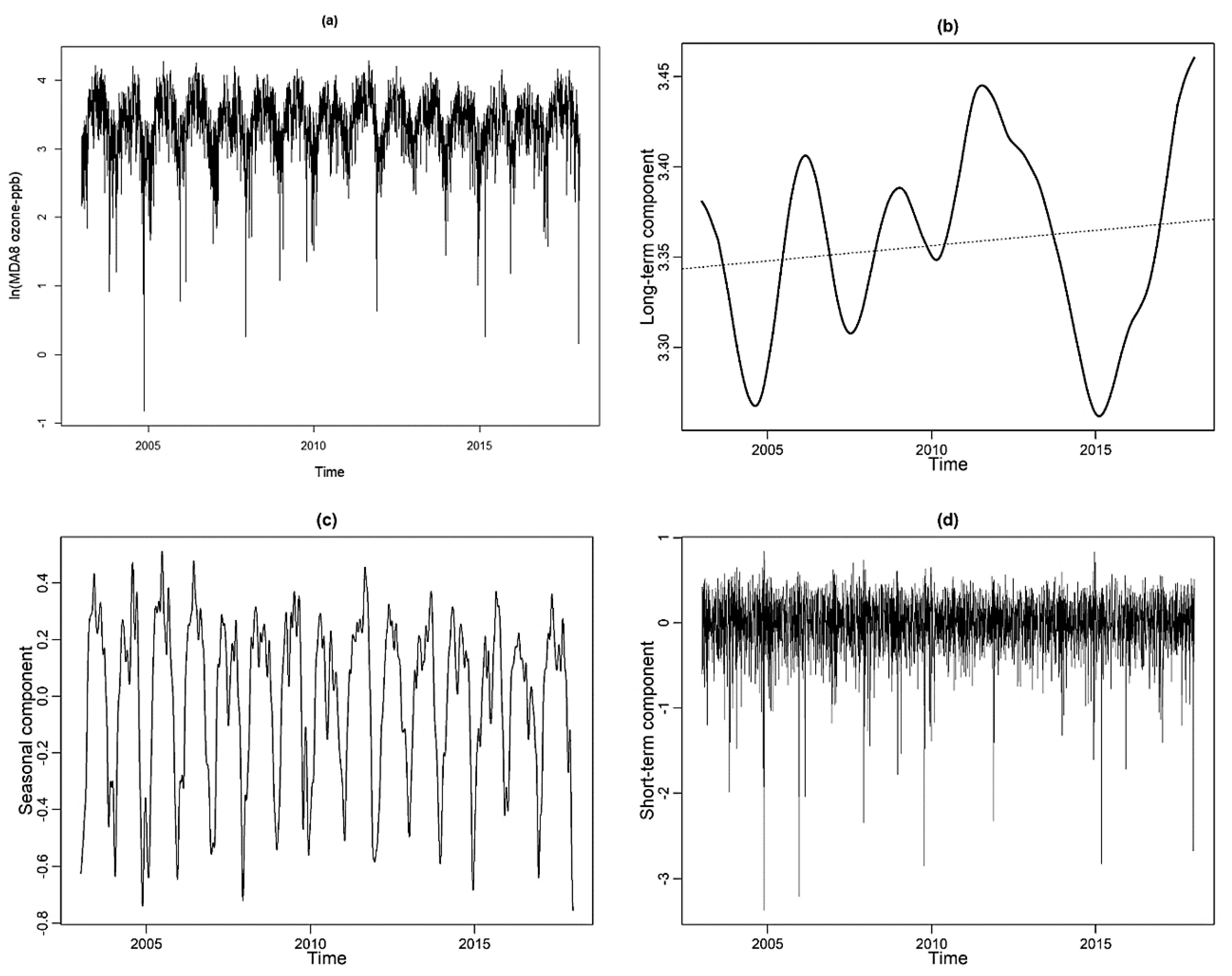
The temporal separation of the natural log of MDA8 ozone concentration was performed for Sites C17, C61, and C402, as shown in Figure 2, Figure 3 and Figure 4, respectively. The original time series plot (Figure 2a showed the more frequent variation with a wide range of ozone concentrations, which are from 0.8 to 4.2 (log scale) at Site C17, −0.2 to 4.0 (log scale) at Site C61, and −0.8 to 4.2 (log scale) in C402. As this plot exhibits a highly variable and frequent change in data series, the trend detection is very difficult. With temporal separation, the plot of long-term (e(t)) component time series had a narrow and stable variation. The long-term component of Site C17 ranged from 3 to 3.4 (log scale), Site C16 ranged from 3 to 3.7 (log scale), and Site C402 ranged from 3.1 to 3.3 (log scale). The trend of the long-term component was ever-increasing at all three sites. The plot exhibited four rising and falling cycles at Sites C17 and C61, but three cycles at Site C402 for the 15 years. The plot of the long-term component defined the data trend more clearly, and hence validated the importance of temporal separation. Multiple peaks were observed annually during the summer in the seasonal component S(t) of MDA8 ozone data, explaining the occurrence of multiple high ozone levels in the area during summer. It also exhibited the three high ozone level episodes that happened in 2007, 2008, and 2009 at Sites C17 and C61, whereas three to four episodes of high ozone were observed during the summer of years 2005, 2008, 2009, and 2017. The highest value was observed in 2005, and the lowest value was in 2017 for Sites C17 and C61; however, 2007 and 2016 years had lower peak ozone concentration than other years at Site C402. The short-term component W(t) of MDA8 ozone concentration was highly frequent and had a wide range of variation. It ranged from −3.6 to 0.8 (log scale) at Site C17, −2.8 to 0.8 (log scale) at C61 and −3.3 to 1.1 (log scale) at C402. The variation was more in minimum values than in the peak values.

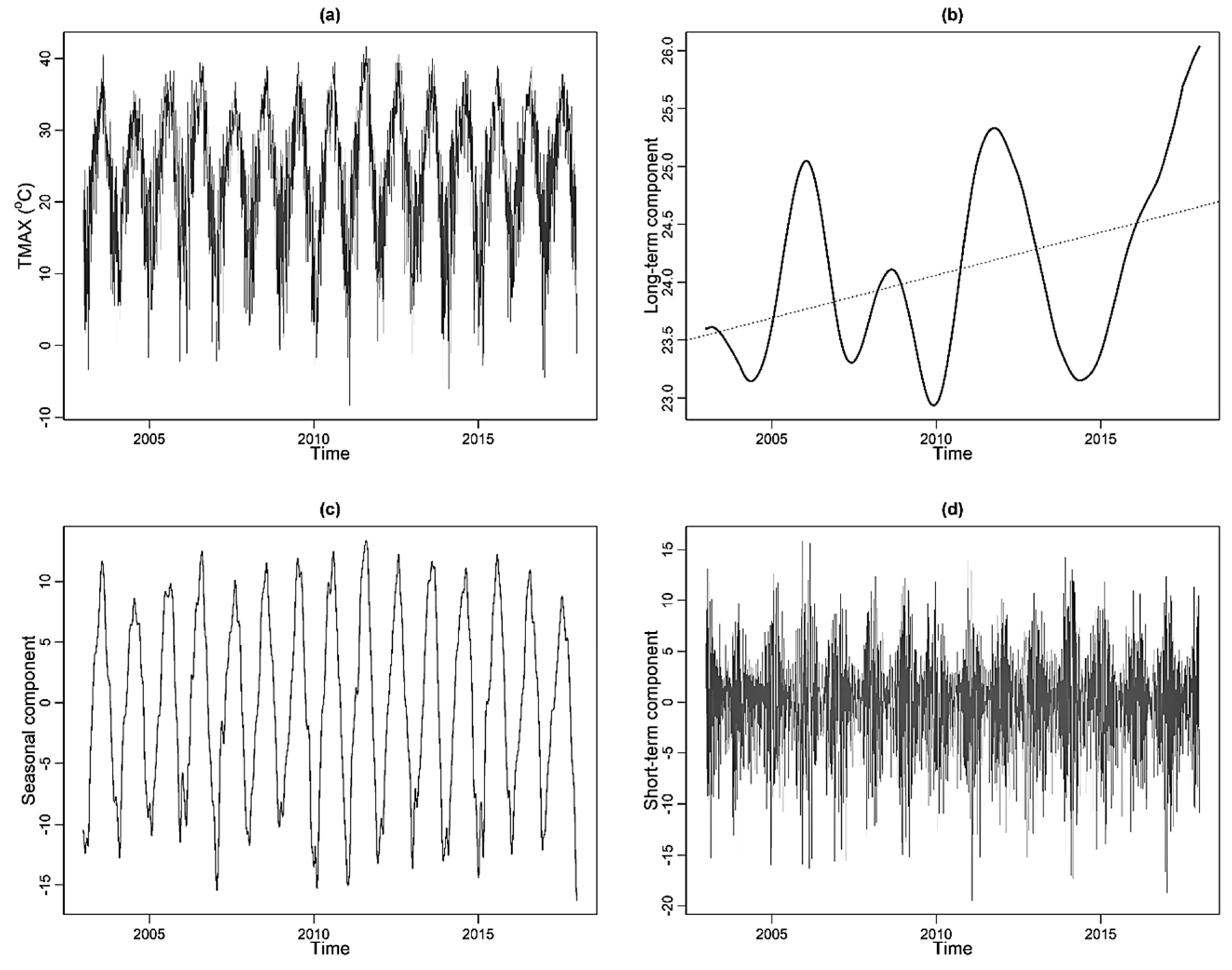
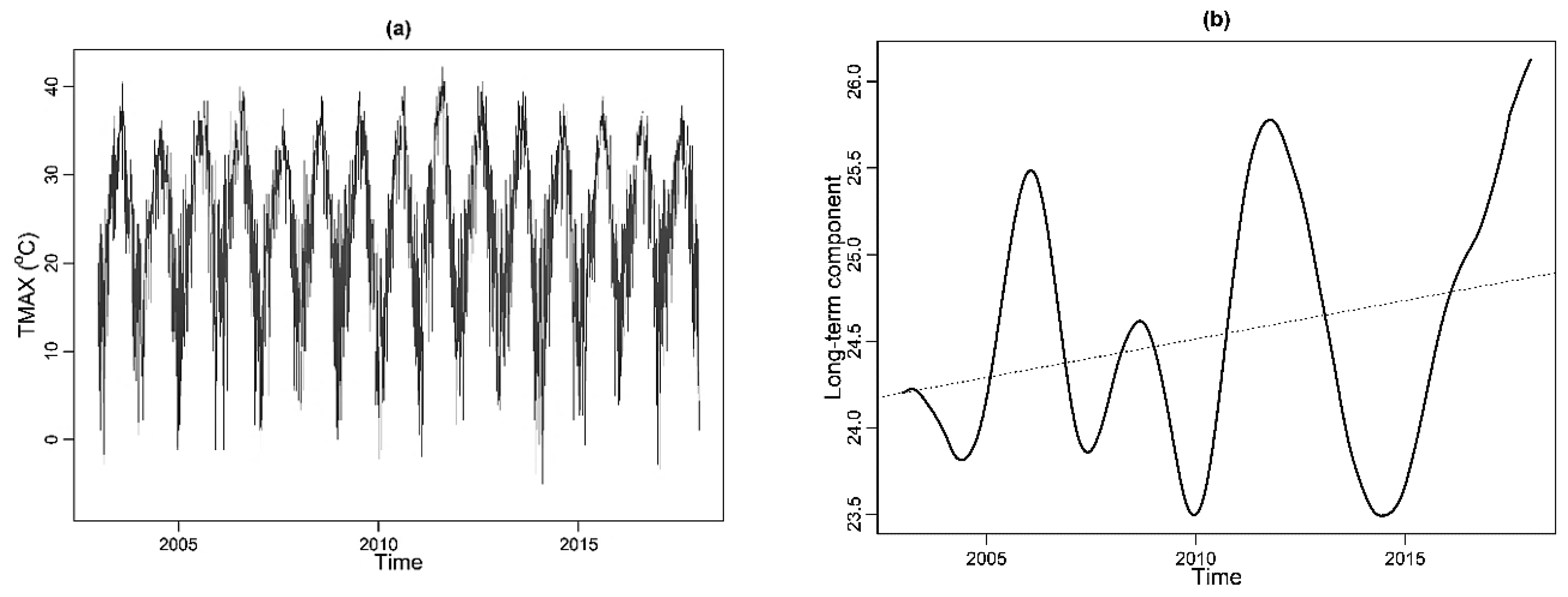
Similarly, the temporal separation of daily maximum temperature and solar radiation was performed for Sites C17, C61, and C402, as shown in Figure 5, Figure 6 and Figure 7, respectively. The temporal separation provided a clearer trend for the long-term component with fewer noises than the original series similar to the ozone data series. The raw temperature data series ranged from −8 to 41 °C at Site C17, −8 to 41 °C at C61, and −8 to 42 °C at C402. After the KZ filtration, they were narrowed down to ranges from 23 to 26 °C in C17, 23.5 to 26.2 °C in C61, and 23.2 to 27 °C in C402 in long-term components. The linear trend of the long-term component showed the increasing trend of temperature. There were four major peaks in 15 years, with the highest peak in 2017 and the lowest in 2003 at Sites C17 and C61, whereas the highest value was observed in 2006 and the lowest in 2010 at Site C402. The plot of the seasonal component showed multiple high and low-temperature episodes each year with a range from −16 to 11 °C in C17, −16 to 13 °C in C61, and −16 to 12 °C at Site C402. The short-term component of temperature was highly variable, which was more in the minimum values. The range values of temporal components of temperature time series at all three sites are very close.

The temporal separations of daily average solar radiation are shown in Figure 8, Figure 9 and Figure 10. The original data series had the fluctuation range from 0 to 380 w/m² at Site C17, 0 to 400 w/m² at C61, and 0 to 400 w/m² at C402. The year 2009 had a single spike of solar radiation level with the highest value of 380 w/m² at C17, whereas C61 had the highest solar radiation observed in 2010 and the highest value at Site C402 in 2016. The long-term component of solar radiation ranged from 166 to 200 w/m² at C17, 166 to 195 w/m² at C61, and 168 to 213 w/m² at C402, a much more narrow range than the original data series. The linear trend showed that the long-term component was in a decreasing trend over the study period in all sites. There were five peaks observed with the lowest value in 2004 at Sites C17 and C61. Site C402 had the lowest value in 2015. The highest value was observed in 2006 at all the sites. The seasonal component of solar radiation showed a couple of peaks in the summertime of every year, similar to the seasonal ozone series. The seasonal component ranged from −120 to 110 w/m² at C17, −120 to 110 w/m² at C61, and −110 to 110 w/m² at C402 with double peaks in most years. Years 2007 and 2014 showed comparatively lower maximum values. The year 2015 had the highest seasonal component. The short-term component exhibited highly variable and noisy series with value ranged from −200 w/m² to 150 w/m² at C17, −210 w/m² to 100 w/m² at C61 and −200 to 200 w/m² at C402.

3.2. Variance Analysis

The variance measured the average of the squared differences from the mean. The smaller the value of variation, the narrower the spread of data, and vice versa. In this study, the contribution of temporal components in the total variation was calculated to see which component led more to data variation. The percentage contribution was calculated using Equation (10). The sum of the percentage variation of temporal components was not 100%, as shown in

Table 1. Contribution of temporal components towards the total variation for three sites.

Parameters	Long Term Component, e(t)	Seasonal Component, s(t)	Short-Term Component, W(t)
Site C17
MDA8 ozone	1.20%	36.83%	41.86%
TMAX	0.75%	71.00%	24.08%
DASR	0.77%	55.44%	39.26%
DAWSR	0.68%	14.79%	68.27%
DAWSS	0.72%	14.76%	68.26%
Site C61
MDA8 ozone	1.78%	36.87%	54.59%
TMAX	0.63%	71.81%	22.96%
DASR	0.45%	55.41%	39.88%
DAWSR	0.69%	15.17%	79.12%
DAWSS	0.72%	14.94%	79.30%
Site C402
MDA8 ozone	1.56%	37.16%	54.13%
TMAX	1.42%	71.96%	22.88%
DASR	1.70%	52.03%	30.76%
DAWSR	1.75%	20.09%	77.75%
DAWSS	1.78%	17.34%	78.18%

. The remaining portion of the variance was contributed by the sum of co-variances, which was considered negligible in this study [19]. A similar trend was observed in all three sites. The long-term component had a negligible (less than 2%) contribution to the overall variation. The seasonal component was dominated by the total variation of solar radiation and temperature. However, the short-term component was significantly dominant in the total variance of wind speed. The short-term component was slightly more dominant than a seasonal component on the total variation of MDA8 ozone data for all sites.

At Site C17, the seasonal component had 55.44% and 71.00% contributions to the total variation of solar radiation and temperature, respectively. The short-term component was more dominant in the total variance of wind speed, with 68.26% contribution and MDA8 ozone with 41.86% contribution at C17, as shown in Table 1. A similar trend had been found at site C61 and site C402. The seasonal component was dominant in the total variation of maximum daily temperature (71.81%), and daily average solar radiation (55.41%) and short-term component are dominant in the total variance of the MDA8 ozone (54.59%) and daily average wind speed (79.3%) at C61. At C402, the seasonal component had the most contribution to the total variance of maximum daily temperature (71.96%) and daily average solar radiation (52.03%). The short-term component had the bigger contribution (54.13%) to the total variation of MDA8 ozone and daily average wind speed (78.18%), as shown in Table 1.

The temporal separation performed by Milanchus, Trivikrama Rao, and Zurbenko (1998) studied the long-term trend of ozone in Cliffside Park, Washington, Chicago, and Los Angeles. These studies indicated that the seasonal component was the primary contributor to the total variance of MDA8 ozone, TMAX and solar radiation, and that the short-term was the primary contributor for wind speed [9]. Another study performed by Botlaguduru et al. (2018) in the Aldine Houston area showed that the short-term component was the primary contributor for MDA8 ozone (63%), Solar Radiation (49%) and wind speed (72%), and the TMAX seasonal component had the highest share (70%) [17]. Differing from these studies, The DFW analysis showed that the short-term component was the primary contributor to the total variance of the MDA8 Ozone time series and wind speed time series. In contrast, the seasonal component was the dominant contributor to the total variance of the TMAX and solar radiation.

3.3. Regression Analysis

The single and multiple linear regression analysis was performed among the original, baseline, and short-term components of MDA8 ozone and meteorological components for each site. The combinations of temperature and solar radiation, temperature and wind speed, solar radiation and wind speed, and the combination of temperature, solar radiation, and wind speed were regressed with MDA8ozone. The coefficient of determination (R²) was calculated for each regression analysis and presented in

Table 2. The coefficient of determination (R²).

Parameter	Raw Data	Base Line	Short Term
Site C17
TMAX	0.331	0.618	0.088
DASR	0.393	0.717	0.147
DAWSR	0.003	0.018	0.023
TMAX/DASR/DAWS	0.447	0.739	0.197
Site C61
TMAX	0.272	0.540	0.084
DASR	0.316	0.640	0.116
DAWSR	0.009	0.004	0.029
TMAX/DASR/DAWS	0.383	0.699	0.188
Site C402
TMAX	0.277	0.534	0.099
DASR	0.336	0.68	0.127
DAWSR	0.012	0.004	0.0318
TMAX/DASR/DAWS	0.393	0.703	0.212

. The result shows that the baseline components of the MDA8 ozone data had a higher correlation with baseline components of TMAX, DASR, and DAWS than the correlation of raw data and short-term components of MDA8, TMAX, DASR, and DAWS.

At Site C17, the result showed that the highest R² value (0.717) was obtained from the correlation of daily average solar radiation with the baseline component of MDA8 ozone. A similar strong correlation was exhibited between TMAX and the baseline component of MDA8 ozone data with an R² value of 0.618, as shown in Table 2. Whereas the weaker correlation was found between meteorological variables and raw MDA8 ozone data. The correlation was comparatively weaker at Site C61 than at Site C17. At site C61, the strongest correlation was exhibited by solar radiation (0.64), followed by temperature (0.54) with the baseline components of the MDA8 ozone data.

Similarly, in C402, baseline components of TMAX (0.53) and DASR (0.68) had a higher correlation with the baseline component of MDA8 ozone than raw and short-term components. The R² value (0.33) of the correlation between raw data of DASR and raw MDA8 ozone was weaker than the correlation between baseline components of DASR and baseline component of MDA8 ozone (0.68). The negligible relation was exhibited by meteorological variables with the short-term components of the MDA8 ozone data. The combination of meteorological variables had improved the correlation values with MDA8 ozone (both raw data and baseline components). The combination of all variables (TMAX, DASR, and DAWS) could only explain 45% of the variability in the raw ozone data, which was improved to 74% in the baseline component with the removal of short-term components from the time series data at Site C17. At C61 and C402, almost 70% of variables could be explained with the combination of the KZ filtered data, whereas only 38% of variables could be defined with the raw MDA8 ozone data. It validated the use of the KZ filter for the evaluation of the role of meteorological parameters in the ozone variation.

From the regression analysis, MDA8 ozone was positively correlated with the baseline components of maximum temperature (TMAX) and daily average solar radiation, as shown in Figure 11i–iii(a,b), respectively, for all three sites. In contrast, the daily average wind speed (DAWS) was negatively correlated with MDA8 ozone for baseline components of the data, as shown in Figure 11i–iii(c) for all sites. For Sites C61 and C402, the MDA8 ozone had a similar correlation as C17 as shown in Figure 11i–iii. The TMAX and daily average solar radiation were positively correlated with MDA8 ozone, as shown in Figure 11i–iii(a,b), but negatively correlated with wind speed as shown in Figure 11i–iii(c). When the relationship between the unadjusted variables and air quality was considered, Wise and Comrie’s (2005) study performed at some sites in Tuscon, AZ, showed that TMAX, Solar Radiation, and wind speed had a positive correlation with MDA8 ozone [10]. Whereas, the study performed by Botlaguduru et al. (2018) in Aldine, Houston, showed that baseline components of MDA8 ozone was positively correlated with baseline components of TMAX and Solar Radiation, and was negatively correlated with baseline components of wind speed, which matches the result of this study [17]. In a recent study, Kotsakis et al. (2019) pointed out that the regional wind carries pollutants from Houston and the Barnett Shale to DFW, and exacerbates DFW ozone concentrations [20].

3.4. Meteorological Adjustment

As suggested by Astitha et al. (2017), the long-term component was dominant on the maximum values of ozone levels [21]. This study had performed a long-term trend analysis with the detrending of meteorological parameters. The long-term series was developed based on a series of residuals from the regression analysis. They did not represent the actual MDA8 ozone series. Equation (14) was used to convert residual long-term series to the actual long-term MDA8 ozone series. Figure 12, Figure 13 and Figure 14 demonstrate the comparison of the adjusted MDA8 long-term component series to the unadjusted long-term series at Keller (C17), Arlington (C61), and Redbird (C402), respectively. The long-term average was plotted in each graph to compare the adjusted and unadjusted series. After meteorological adjustment of MDA8 ozone long-term series, linear trends were developed for all sites from the linear regression analysis, as shown in

Table 3. Estimated linear trends for long-term meteorologically independent MDA8 ozone (ppb/yr).

Model	MDA8 Ozone Linear Trend (ppb/Year)
	Keller (C17)	Arlington (C61)	Redbird (C402)
Model 1 (TMAX)	0.007 ± 0.006; R2 = 0.001	0.001 ± 0.007; R2 = 0.001	0.161 ± 0.008; R2 = 0.224
Model 2 (DASR)	0.076 ± 0.006; R2 = 0.104	0.01 ± 0.007; R2 = 0.001	0.248 ± 0.006; R2 = 0.567
Model 3 (DAWS)	0.016 ± 0.009; R2 = 0.002	0.014 ± 0.009; R2 = 0.001	0.044 ± 0.011; R2 = 0.010
Model 4 (TMAX/DASR/DAWS)	0.072 ± 0.006; R2 = 0.107	0.019 ± 0.007; R2 = 0.005	0.19 ± 0.006; R2 = 0.398

.

At site C17, temperature (TMAX) and daily average solar radiation (DASR) were positively correlated with the unadjusted long-term component of MDA8 ozone, as shown in Figure 12a,b. When there was lower than average TMAX, the adjusted trend was above the unadjusted trend, and when the TMAX was higher than the average value, the adjusted trends were pushed lower than the unadjusted trend. For example, from the beginning of 2003 to 2005, the adjusted trend line was higher than the unadjusted with TMAX lower than the average TMAX. A similar correlation was found with solar radiation as well. The linear trend of the adjusted ozone was evaluated using linear regression and found the very low R² value (0.001) for model 1, as shown in Table 3. It exhibited that linearity was not applicable for model 1 at the sites C71 and C61. In contrast, the adjusted trend of ozone without the influence of temperature exhibited the increasing linear trend with a significant R² value (0.161 ± 0.008; R² = 0.224; p-value < 0.5). With the variation in the TMAX value, the gap between the adjusted and unadjusted trend lines was significant. Hence, the adjustment of TMAX in the MDA8 ozone had an important role in the ozone trend analysis.

The adjustment of the long-term component of MDA8 ozone with the removal of daily average solar radiation (DASR) is shown in Figure 12b, Figure 13b, and Figure 14b. The linear trend of the long-term component of MDA8 ozone after removal of the solar radiation forcing was not signifcant over the study period for C17 and C61. The low R² value in the model 2 for the MDA8 ozone of site C17 (0.076 ± 0.006; R² = 0.104; p-value < 0.5) and site C61 (0.01 ± 0.007; R² = 0.001; p-value < 0.5) demonstrates the weak linearity. A strong linear trend was observed at the site C402 with significant R² value (0.248 ± 0.006; R² = 0.567; p-value < 0.5). Similar to temperature (model 1), the solar radiation adjustment (model 2) would help to define a better ozone trend. However, in contrast to temperature and solar radiation, the wind speed (model 3) was negatively correlated with an unadjusted long-term component of MDA8 ozone. The linear trend analysis for model 3 showed the weak linearity with a mild increasing trend for all sites, as shown in Table 3.

Figure 12d, Figure 13d, and Figure 14d explain the result of model 4, which explained the comparison of the unadjusted trend of the MDA8 ozone long-term component to the trend of the fully adjusted long-term component of MDA8 ozone. With the removal of the influence of TMAX, DASR, DAWS, the variation range of long-term component of MDA8 ozone (6 ppb/yr) had been narrowed down to the range of 3 ppb/yr, as shown in Figure 12d. The linearity analysis of model 4 for the site C17 resulted in the low R² value and slightly increasing trend (0.072 ± 0.006; R² = 0.107, p-value < 0.5) of the long-term component of the MDA8 ozone. The result was similar for the site C61 with the R² value 0.005 and a slope of 0.019. In comparison, strong linearity with the increasing trend was observed for the long-term component of the MDA8 ozone at site C402 with R² value 0.398 and slope 0.19, as shown in Figure 14d and Table 3 (model 4). A higher degree of determinacy (R² value) and strong linearity were observed with the removal of multiple meteorological parameters (TMAX, DASR, DAWS) than the adjustment of individual parameters, as shown in Table 3. The highest R² value for each site was observed for model 4. In contrast to our study, the decreasing trend (0.412 ± 0.007) was observed in a study performed in the Houston area [17].

The comparison of a long-term component trend of MDA8 ozone among all sites is presented in Figure 15. The long-term component of the MDA8 ozone time series had an increasing trend from 2003 to 2017 for all sites. Site C402 had a higher increasing trend than the sites C17 and C61. The decrease in ozone concentration was expected over time due to stringent emission standards by USEPA. However, the slightly increasing trend for the long-term MDA8 ozone can be justified by the strong increasing trend of VOCs and NOx in the DFW area. It is in agreement with the generally upward trend of tropospheric ozone, which influences the surface ozone background, and the generally downward trend of NO_x emissions in the point resources of the USA, leading to ozone destruction in the first place and subsequently to an increase of ozone [22].

3.5. Role of NOx/VOC Emissions and Texas State Implementation Plan

NOx and VOC emissions are the primary precursors of ozone formation. The study showed a slightly increasing trend of long-term ozone component after meteorological adjustment. The detection of the influence of NOx and VOC on the increasing trend of long-term ozone component is key before concluding. The trend analysis of NOx and VOC emissions in pounds per day (PP was performed using the emission inventory list of Texas for point and non-point sources presented in Figure 16, respectively. Figure 16A,B exhibited the emission trends of NOx and VOC during the ozone season, and Figure 16C,D represented the annual emission trends of NOx and VOC. Due to the data limitation, the emission data in 2017 is not present in Figure 16.

From the analysis of the emission inventory list of a point source, it can be concluded that NOx emissions had been decreasing significantly in both data sets (ozone season and annual). A similar trend was identified in VOC emissions during the ozone season (March to November for Dallas County), i.e., spring, summer, and autumn. This decreasing trend was due to the state implementation plan (SIP) as reasonable further progress (RFP). State Implementation Plan in the DFW area (Region 4) set the target to achieve the 15% reduction of NO_x and VOCs from 2002 to 2008. Instead, mobile source emission analysis showed a significant increasing trend of VOCs and NOx, as shown in Figure 17. Mobile source emission analysis was done from 2002 to 2014 National Emissions Inventory (NEI) for Texas state considering every three years. Due to the data limitation, the emission data in 2017 is not present in Figure 17.

Even though point-source emissions showed a decreasing trend, the strong increasing trend of VOCs and NOx emissions from mobile sources validated the increasing trend of the long-term ozone component for the study area.

4. Conclusions

The study was performed for three sites, Keller (Station C17), Redbird (Station C402), and Arlington (C61) of DFW. The sites were selected mainly based on the dominant land use of the area and data availability. The MDA8 ozone time series, daily maximum temperature, daily average solar radiation, and daily average wind speed data were considered for the study. The time-series data were separated using the KZ filter into three components, i.e., long-term components, seasonal components, and short-term components. Then the role of each component on the total variation of data was identified. The single and multiple regression analysis was performed to identify the relationship of meteorological variables to the raw ozone data and baseline ozone data. The overall linear trend analysis was done for each site, MDA8 ozone data. The study found that the temporal separation of time series data is useful to identify a clear trend with the filtering out of noise in the data. A long-term component provided a smooth trend, whereas the seasonal component assisted in the quantification of the seasonal forcing on ozone concentrations. From the study of the contribution of each temporal component in the total variation of the raw data, it was observed that the seasonal component was dominant in the total variation of TMAX and DASR. In contrast, the short-term component was dominant in the total variance of the MDA8 ozone and DAWS for all three sites. The contribution of long-term components in the total variation was negligible. It was suggested that the TMAX and DASR had a major effect on the regional ozone formation. The correlation of MDA8 ozone with the meteorological components (TMAX, DASR, and DAWS) was observed using regression analysis. The regression analysis was performed for each of the temporal components (long-term, seasonal and short-term) that showed the baseline component bears the highest correlation, and when we evaluated the correlation among them, the solar radiation had the highest correlation to the MDA8 ozone followed by temperature.

The combined effect of all meteorological variables (TMAX, DASR, and DAWS) defined the correlation more strongly with baseline data than raw data. The meteorological adjustment analysis showed that long-term MDA8 ozone had a significant increasing trend (0.19 ± 0.006 ppb/y) at the Redbird (C402) site. However, for the other two sites—Keller (C17) and Arlington (C61)—the meteorologically adjusted MDA8 ozone levels were relatively stable. During the same period of 2003–2017, the analysis of emission inventory for the point-sources suggests that the quantum of NOx and VOC emissions had reduced considerably. A corresponding decrease in ozone levels could not be attained due to the increase in NOx and VOC emissions from mobile sources. This study indicates that an increased regulatory attention may be required for controlling ozone precursors from mobile sources in order to achieve any substantial reduction in the long-term ozone levels in the DFW region.